Global non-axisymmetric perturbation configurations in a composite disc system with an isopedic magnetic field:
relation between dark matter halo and magnetic field

Abstract

We study global non-axisymmetric stationary perturbations of aligned and unaligned logarithmic spiral configurations in an axisymmetric composite differentially rotating disc system of scale-free stellar and isopedically magnetized gas discs coupled by gravity. The infinitely thin gas disc is threaded across by a vertical magnetic field $B_{z}$ with a constant dimensionless isopedic ratio $\lambda\equiv 2\pi\sqrt{G}\Sigma^{(g)}/B_{z}$ of surface gas mass density $\Sigma^{(g)}$ to $B_{z}$ with $G$ being the gravitational constant. Our exploration focuses on the relation between the isopedic ratio $\lambda$ and the dark matter amount represented by a gravitational potential ratio $f\equiv\overline{\Phi}/\Phi$ in order to sustain stationary perturbation configurations, where $\overline{\Phi}$ is the gravitational potential of a presumed axisymmetric halo of dark matter and $\Phi$ is the gravitational potential of the composite disc matter. For typical disc galaxies, we explore relevant parameter ranges numerically. High and low $\lambda$ values correspond to relatively weak and strong magnetic fields given the same gas surface mass density, respectively. The main goal of our model analysis is to reveal the relation between isopedic magnetic fields and dark matter halo in spiral galaxies with globally stationary perturbation configurations. Our results show that for stationary perturbation configurations, fairly strong yet realistic magnetic fields require a considerably larger amount of dark matter in aligned and unaligned cases than weak or moderate magnetic field strengths. We discuss astrophysical and cosmological implications of our findings. For examples, patterns and pattern speeds of galaxies may change during the course of galactic evolution. Multiple-armed galaxies may be more numerous in the early Universe. Flocculent galaxies may represent the transitional phase of pattern variations in galaxies.

1 Introduction

Since the seminal studies of the galactic density wave theory in the 1960’s pioneered by Lin & Shu (1964, 1966), many advanced works have been done to describe the large-scale dynamics of ‘grand-design’ spiral structures in disc galaxies. In terms of theoretical development, it is natural to first concentrate on linear perturbation theories. As synchrotron radio observations have revealed since the early 1970’s that magnetic fields are ubiquitous in disc galaxies (e.g. Sofue, Fujimoto & Wielebinski 1986; Beck et al. 1996; Zweibel & Heiles 1997; Brown, Taylor, Wielebinski & Mueller 2003), magnetic fields have been recognized as an important aspect in the model treatment of spiral galaxies and thus the magnetohydrodynamic (MHD) density wave theory was developed (Fan & Lou 1996; Lou & Fan 1998). Over the past decade, a research area has been developed on the so-called scale-free discs and perturbation structures therein (e.g. Syer & Tremaine 1996; Shu et al. 2000; Shen & Lou 2004; Lou & Zou 2004; Shen, Liu & Lou 2005; Lou & Zou 2006; Wu & Lou 2006; Lou & Bai 2006). The scale-free condition corresponds to a power-law dependence of all physical quantities on the cylindrical radius $r$, for example, the background surface mass density is $\Sigma_{0}\propto r^{-2\beta-1}$ with $\beta$ being a constant scaling index. Such analysis was first initiated for relatively simple models of only one gas disc. We are now able to explore a composite system of a stellar disc and an isopedically magnetized gas disc embedded in a dark matter halo. For this overall configuration, we study possible large-scale perturbation structures and stationary MHD density waves. To simplify the mathematical treatment, the stellar disc is approximated as a fluid and the magnetized gaseous disc as a magnetofluid and both are assumed to be geometrically razor-thin and scale-free discs. In general situations, the scaling exponent $\beta$ may vary radially in a certain range for different disc galaxies. For more or less flat rotation curves which can be grossly determined in many spiral galaxies from large radii to the centre (e.g. Rubin 1965; Roberts & Rots 1973; Krumm & Salpeter 1976, 1977; Bosma 1981; Kent 1986, 1987, 1988), index $\beta$ may be regarded as almost zero. According to the classical Newtonian gravity theory, a significantly larger amount of mass than the visible mass of the disc is needed in order to sustain observed grossly flat rotation curves. As a consequence of this discrepancy between the visible and the required mass as well as the disc stability property, the presence of a massive dark matter halo has been proposed (e.g. Ostriker & Peebles 1973; Ostriker et al. 1974; Binney & Tremaine 1987). Nowadays, the inclusion of a massive axisymmetric dark matter halo is a common practice for studying large-scale galactic dynamics.

Meanwhile, observations of disc galaxies nowadays can be used to estimate open magnetic field strengths and configurations on both sides of a galactic disc plane. While these open magnetic fields are most certainly interlaced with closed coplanar magnetic fields, at this stage of our theoretical model development, we consider only open magnetic field crossing the disc plane almost vertically. Shu & Li (1997) introduced the so-called isopedic condition of $B_{z}(r,\ \theta,\ t)\propto\Sigma^{(g)}$ where $B_{z}$ is the $z-$component of the magnetic field and $\Sigma^{(g)}$ is the gas disc surface mass density. The ratio $\Sigma^{(g)}/B_{z}$ thus remains constant in time and space. This situation is referred to as the isopedic magnetic field configuration. In fact, this constant ratio can be actually inferred by the magnetic field-freezing effect according to the ideal magnetohydrodynamic (MHD) equations (Lou & Wu 2005). Effective modifications to the gravitational potential and the gas pressure are derived in Shu & Li (1997) for a single isopedically magnetized gas disc. This isopedic condition was first proposed as an ansatz based on numerical simulations of magnetized cloud core formation through ambipolar diffusions (e.g. Nakano 1979; Lizano & Shu 1989; and references cited in Shu & Li 1997). On the basis of earlier work of Shu & Li (1997), Lou & Wu (2005) generalize their results into theorems for two gravitationally coupled discs where only the gas disc is isopedically magnetized. Moreover, they actually demonstrate that a constant ratio $\lambda=2\pi\sqrt{G}\Sigma^{(g)}/B_{z}$, with $G$ being the gravitational constant, can be proved as a consequence of frozen-in condition by the standard ideal nonlinear MHD equations. In this model analysis, we shall adopt the same expressions of Lou & Wu (2005) for the effect of an isopedic magnetic field anchored in the gas disc component.

In order to catch the essence of MHD density wave equations from analytical and numerical explorations, a few assumptions and simplifications are invoked such as the stationary condition in our frame of reference. As first advanced and hypothesized by Lin & Shu (1966), the quasi-stationary spiral structure (QSSS) has been studied since the early 1960’s (e.g. Bertin & Lin 1996 and extensive references therein). There the pattern speed of density wave travels very slowly as compared to the differential rotation speed $v_{\theta}$ of the disc matter. Our stationary requirement can be simply regarded as a limiting case of the QSSS approximation. Based on observations of the nearby spiral galaxy M81, Visser (1980a, b) has shown that the density wave theory does indeed account for gross aspects of the large-scale dynamics of this spiral galaxy.

Kendall et al. (2008) presented further observational data analysis of the nearby galaxy M81, where the large-scale spatial offset between the (old) stellar spiral wave and the gas shock front was examined. Theoretical considerations (e.g. Gittins & Clarke 2004; Chakrabarti 2008) have shown that the offset between the gas shock front (i.e. the maximum gas density) and the spiral potential minimum (determined by the spiral pattern in the old stellar disc component) may yield clues about the lifetime of a spiral pattern. By comparing observational results with the predictions of Gittins & Clarke (2004), Kendall et al. (2008) found that the galaxy M81 probably possesses a long-lived spiral pattern. Very recently, Chakrabarti (2008) performed numerical simulations to demonstrate that an angular momentum transport takes place from gas to stars in a composite system, leading to an approximately time-steady spiral structure in the stellar disc component (treated as collisionless N-body particles). A major part that plays an important role is the relatively cold gas disc particles modelled by smoothed particle hydrodynamic (SPH) and is dissipative due to an artificial viscosity. Regarding the spiral structure in the gaseous disc component, Chakrabarti et al. (2003) have shown, that the so-called ultraharmonic resonances that the gas experiences in a fixed stellar spiral potential can lead to highly time-dependent gas responses, not allowing long-lived spiral patterns in the gas disc. In our model of a composite disc system, there is no fixed stellar potential but rather stellar and gaseous discs are gravitationally coupled to each other in terms of dynamical adjustment. While the simulation results reveal only a long-lived stellar spiral pattern, for our semi-analytical calculations, a stationary requirement for both spiral patterns in stellar and gaseous discs may be imposed without inconsistency. This offers a useful construct for modelling large-scale patterns in isopedically magnetized spiral galaxies.

Theoretically, two classes of stationary MHD density wave solutions with in-phase and out-of-phase density perturbations are expected to exist in a composite disc system according to Lou & Shen (2003). The physical reason for these two different couplings between the stellar and gaseous discs is a dynamic interplay between star formation and gas clumping processes (Shen & Lou 2004). When the surface mass densities are out of phase, the self-gravity of the composite disc system is reduced. The azimuthal propagation of density wave is therefore faster and if a stationary configuration is desired, then the disc should rotate faster. When the surface mass densities are in phase, the self-gravity is enhanced. The azimuthal propagation of the density wave is slower and the disc should then rotate slower in order to maintain a stationary configuration (Lou & Shen 2003).

Our present investigation mainly focuses on the variation of the amount of dark matter in the halo needed to sustain stationary perturbation configurations as the isopedic magnetic field strength varies. Therefore, we use typical values of disc galaxies for different parameters such as the ‘sound speed’ or the surface mass density. By invoking several physical requirements for the dark matter halo such as a non-negative potential ratio and so forth, the physical parameter range of stationary perturbation solutions can be identified.

In Section 2, the problem formulation, the basic formulae and the coupled fluid and magnetofluid equations for the two discs are presented. In Section 3, we discuss effective modifications to the gravitational potential and the enthalpy in the gas disc when an isopedic magnetic field is introduced. In Section 4, we derive several relevant relations for the background rotational equilibrium configuration. In Section 5, MHD perturbations are introduced and the relevant global stationary dispersion relation is derived. For globally stationary MHD perturbation configurations, we calculate the dark matter amount and discuss which parameters affect this amount. Section 6 describes briefly the values for the parameters adopted for this model analysis. In Section 7, we study aligned cases where perturbations of different radii can be aligned radially. In Section 8, we study unaligned logarithmic spiral cases with a constant radial flux of angular momentum. Such unaligned cases have MHD perturbations which are systematically phase shifted azimuthally as a function of radius $r$. In unaligned cases, MHD density waves propagate in both azimuthal and radial directions. The constant radial flux of angular momentum is realized by setting the perturbation scale-free index $\beta_{1}$ to $1/4$ (e.g. Goldreich & Tremaine 1979; Shen et al. 2005). In Section 9, we discuss two limiting cases of no magnetic field and only a single isopedically magnetized gaseous disc. In the last Section 10, we summarize our work and draw conclusions.

2 Nomenclature and Basic Fluid and Magnetohydrodynamic (MHD) Equations

We first introduce notations for the relevant physical variables used in our model formulation and analysis. We largely adopt the same nomenclature of Wu & Lou (2005) for a model of a single scale-free disc with an isopedic magnetic field. Whenever the superscript $(i)$ is attached to a physical variable, the relevant equation is valid for both stellar $(s)$ and gaseous $(g)$ discs in parallel. Cylindrical coordinates $(r,\ \theta,\ z)$ are adopted for our model formulation and we confine our analysis within the $z=0$ plane for an infinitely thin composite disc system in differential rotation. For example, variable $\Sigma^{(s)}(r,\ \theta,\ t)$ is the two-dimensional surface mass density of the stellar disc and $\Sigma^{(g)}(r,\ \theta,\ t)$ is that of the isopedically magnetized gas disc. The total surface mass density $\Sigma(r,\ \theta,\ t)=\Sigma^{(s)}+\Sigma^{(g)}$ is the sum of these two disc surface mass densities. Two different coplanar bulk flow velocities are possible in the two discs: the radial bulk flow velocity $v^{(i)}_{r}(r,\ \theta,\ t)$ and the azimuthal bulk flow velocity $v^{(i)}_{\theta}(r,\ \theta,\ t)$. For the background rotational equilibrium disc configuration of axisymmetry, the radial flow velocities should vanish. The two-dimensional pressure (i.e. vertically integrated pressure) in each disc is described by $\Pi^{(i)}(r,\ \theta,\ t)$. Between the two-dimensional variables and their three-dimensional counterparts, the following integral relations exist,

$$\Pi^{(i)}(r,\ \theta,\ t)=\int\limits_{\Delta z}p^{(i)}(r,\ \theta,\ z,\ t)dz\hskip 28.45274pt\hbox{ and }\hskip 28.45274pt\Sigma^{(i)}(r,\ \theta,\ t)=\int\limits_{\Delta z}\rho^{(i)}(r,\ \theta,\ z,\ t)dz\ ,$$ (1)

where $p^{(i)}$ is the three-dimensional pressure and $\rho^{(i)}$ is the three-dimensional mass density, and $\Delta z$ is the disc thickness presumed to be very small compared to radius $r$. Thus, $\Pi^{(i)}$ is the vertical integral of pressure $p^{(i)}$. The three-dimensional polytropic equation of state is $p^{(i)}=k^{(i)}_{3}[\rho^{(i)}]^{\gamma}$ with $\gamma$ being the polytropic index and $k^{(i)}_{3}$ being related to the disc entropy. The vertically integrated barotropic equation of state can then be expressed as

$$\Pi^{(i)}=k^{(i)}\left[\Sigma^{(i)}\right]^{n}\ ,$$ (2)

where index $n>0$ is the barotropic index, $k^{(i)}>0$ for a warm disc and $k^{(i)}=0$ for a cold disc. The barotropic sound speed $a^{(i)}$ in each disc is then defined by

$$\left[a^{(i)}\right]^{2}={\mathrm{d}\Pi^{(i)}}\big{/}{\mathrm{d}\Sigma^{(i)}}=nk^{(i)}\left[\Sigma^{(i)}\right]^{n-1}=n\Pi^{(i)}\big{/}\Sigma^{(i)}\ .$$ (3)

The ‘sound speed’ $a^{(s)}$ in the stellar disc is effectively related to the velocity dispersion of stars. The enthalpy $H^{(i)}$ in each disc is given by

$$H^{(i)}=\int\frac{\mathrm{d}\Pi^{(i)}}{\Sigma^{(i)}}=\frac{nk^{(i)}[\Sigma^{(i)}]^{n-1}}{(n-1)}=\frac{[a^{(i)}]^{2}}{(n-1)}\$$ (4)

and is proportional to the square of ‘sound speed’ in each disc. The gravitational coupling between the stellar and magnetized gaseous discs is described by the well-known Poisson integral

$$\Phi(r,\theta,t)=\oint\mathrm{d}\psi\int\frac{-G\Sigma(r^{\prime},\ \psi,\ t)r^{\prime}\mathrm{d}r^{\prime}}{[r^{\prime 2}+r^{2}-2rr^{\prime}\cos(\psi-\theta)]^{1/2}}\ ,$$ (5)

where $G=6.67\times 10^{-8}\hbox{ g}^{-1}\hbox{ cm}^{3}\hbox{ s}^{-2}$ is the gravitational constant. The gravitational potentials of the two discs can be separately written as

$$\Phi^{(s)}(r,\theta,t)=\oint\mathrm{d}\psi\int\frac{-G\Sigma^{(s)}(r^{\prime},\ \psi,\ t)r^{\prime}\mathrm{d}r^{\prime}}{[r^{\prime 2}+r^{2}-2rr^{\prime}\cos(\psi-\theta)]^{1/2}}\ ,\qquad\qquad\Phi^{(g)}(r,\theta,t)=\oint\mathrm{d}\psi\int\frac{-G\Sigma^{(g)}(r^{\prime},\ \psi,\ t)r^{\prime}\mathrm{d}r^{\prime}}{[r^{\prime 2}+r^{2}-2rr^{\prime}\cos(\psi-\theta)]^{1/2}}\ ,$$ (6)

with $\Phi=\Phi^{(s)}+\Phi^{(g)}$. In a disc galaxy, an axisymmetric massive dark matter halo is represented by a gravitational potential $\overline{\Phi}$. A recent numerical exploration (e.g. Diemand et al. 2008) has shown that the dark matter halo is not smooth and uniform, but rather consists of many smaller clumpy subhalos. For simplicity, we assume the dark matter halo to be grossly axisymmetric on large scales and unperturbed in our model analysis at this stage. The composite system of two coupled discs with an axisymmetric dark matter halo is described by coupled nonlinear fluid equations $(\ref{eq:conti})-(\ref{eq:euler2})$ below.

$$\frac{\partial\Sigma^{(i)}}{\partial t}+\frac{1}{r}\frac{\partial}{\partial r}\left[r\Sigma^{(i)}v^{(i)}_{r}\right]+\frac{1}{r}\frac{\partial}{\partial\theta}\left[\Sigma^{(i)}v^{(i)}_{\theta}\right]=0\ ,\qquad\qquad$$ (7)

$$\frac{\partial v^{(i)}_{r}}{\partial t}+v^{(i)}_{r}\frac{\partial v^{(i)}_{r}}{\partial r}+\frac{v^{(i)}_{\theta}}{r}\frac{\partial v^{(i)}_{r}}{\partial\theta}-\frac{\big{[}v^{(i)}_{\theta}\big{]}^{2}}{r}=-\frac{1}{\Sigma^{(i)}}\frac{\partial\Pi^{(i)}}{\partial r}-\frac{\partial(\Phi+\overline{\Phi})}{\partial r}=-\frac{\partial\big{[}H^{(i)}+\Phi+\overline{\Phi}\big{]}}{\partial r}\ ,\qquad\qquad$$ (8)

$$\frac{\partial v^{(i)}_{\theta}}{\partial t}+v^{(i)}_{r}\frac{\partial v^{(i)}_{\theta}}{\partial r}+\frac{v^{(i)}_{\theta}}{r}\frac{\partial v^{(i)}_{\theta}}{\partial\theta}+\frac{v^{(i)}_{\theta}v^{(i)}_{r}}{r}=-\frac{1}{\Sigma^{(i)}}\frac{\partial\Pi^{(i)}}{r\partial\theta}-\frac{\partial(\Phi+\overline{\Phi})}{r\partial\theta}=-\frac{\partial\big{[}H^{(i)}+\Phi+\overline{\Phi}\big{]}}{r\partial\theta}\ \qquad\qquad$$ (9)

(e.g. Shen & Lou 2004). Equation (7) is the mass conservation, and equations (8) and (9) are the radial and azimuthal momentum equations. These fluid equations for both stellar and gaseous discs are confined to the two-dimensional disc plane at $z=0$, while Poisson integral equation (5) is three-dimensional. These equations do not involve an isopedic magnetic field at this stage.

2.1 Scale-Free Discs and Relevant Parameter Ranges

Scale-free discs are represented by power-law forms with a few disc index parameters. We write a self-consistent form of disc solution as

$$v_{r}^{(g)}=e^{(g)}(\varphi)r^{-\beta}\ ,\qquad\qquad v_{r}^{(s)}=e^{(s)}(\varphi)r^{-\beta}\ ,$$ (10)

$$v_{\theta}^{(g)}=b^{(g)}(\varphi)r^{-\beta}\ ,\qquad\qquad v_{\theta}^{(s)}=b^{(s)}(\varphi)r^{-\beta}\ ,$$ (11)

$$\Sigma^{(g)}=S^{(g)}(\varphi)r^{-2\beta-1}\ ,\qquad\qquad\Sigma^{(s)}=S^{(s)}(\varphi)r^{-2\beta-1}\ ,$$ (12)

$$\Pi^{(g)}=k^{(g)}\big{[}\Sigma^{(g)}\big{]}^{n}\ ,\qquad\qquad\Pi^{(s)}=k^{(s)}\big{[}\Sigma^{(s)}\big{]}^{n}\ ,$$ (13)

$$H^{(g)}=Q^{(g)}(\varphi)r^{-2\beta}\ ,\qquad\qquad H^{(s)}=Q^{(s)}(\varphi)r^{-2\beta}\,$$ (14)

$$\Phi=-P(\varphi)r^{-2\beta}\ ,\qquad\qquad\qquad\overline{\Phi}=-\overline{P}r^{-2\beta}\ ,$$ (15)

where $e^{(i)}$, $b^{(i)}$, $S^{(i)}$, $Q^{(i)}$, and $P$ are functions of only $\varphi$ which is an argument abbreviation $\varphi\equiv\theta+\mu\ln r$ with $\mu$ being a parameter, and $\overline{P}$ for the dark matter halo is a constant coefficient independent of $\varphi$. The detailed mathematical procedure of constructing such self-similar scale-free solutions can be found in Lynden-Bell & Lemos (1999). By comparing equations (4) and (14), we immediately obtain a relation between the two power-law indices $n$ and $\beta$, namely

$$(2\beta+1)(n-1)=2\beta\ ,\hskip 14.22636pt\to\hskip 14.22636ptn={(1+4\beta)}/{(1+2\beta)}\ .$$ (16)

Based on expressions (2) and (3), we find that for warm discs with $k^{(i)}>0$, the barotropic index $n$ must also be positive in order to ensure a positive right-hand side (RHS) of equation (3) (i.e. a real sound speed). This physical requirement for warm discs leads to either $\beta>-1/4$ or $\beta<-1/2$. For cold discs with $k^{(i)}\to 0$, there is no constraint on the barotropic index $n$. Another empirical constraint which arises from observational results is that $\Sigma^{(i)}$ should decrease with increasing $r$ which requires a $\beta$ larger than $-1/2$. With the assumption of decreasing $\Sigma^{(i)}$, a singularity of mass would arise in the central region as $r\rightarrow 0^{+}$. This problem can be remedied by requiring a finite integral

$$\lim_{r\to 0}\int_{0}^{r}\int_{0}^{2\pi}\Sigma^{(i)}(r,\theta)r\mathrm{d}r\mathrm{d}\theta=\int_{0}^{2\pi}S^{(i)}(\theta)\mathrm{d}\theta\lim_{r\to 0}\left[\frac{r^{1-2\beta}}{1-2\beta}\right]_{0}^{r}<+\infty\$$ (17)

and this then leads to $\beta<1/2$. Therefore for warm discs with $k^{(i)}>0$, the scaling index range is $\beta\in(-1/4,\ 1/2)$ and for cold discs with $k^{(i)}=0$, we simply require $\beta\in(-1/2,\ 1/2)$.

3 An Isopedic magnetic field across a scale-free thin gaseous disc

Effective modifications of the gravitational potential and the pressure in a composite system of two discs due to the very presence of an isopedic magnetic field were derived in reference to the study of singular isothermal discs (SIDs) by Lou & Wu (2005). SIDs represent only a special class (i.e. $\beta=0$) of scale-free discs in our more general formalism here. We now briefly summarize their results and introduce the relevant variables in the current model context. Following Li & Shu (1996), we define a constant dimensionless ratio $\lambda$ as

$$\lambda=2\pi G^{1/2}\Sigma^{(g)}/B_{z}\equiv 2\pi G^{1/2}\Lambda=\mathrm{constant}>0\ .$$ (18)

Parameters $\lambda$ and $\Lambda$ indicate how strong the magnetic field is as compared to the surface mass density of the gas disc; they are proportional to $B_{z}^{-1}$ such that for weak or strong magnetic fields they become very large or small, respectively. Parameter $\eta$ is a dimensionless ratio of the total horizontal gravitational acceleration $|\vec{f}_{\parallel}|=|\vec{f}^{(g)}_{\parallel}+\vec{f}^{(s)}_{\parallel}|$ (continuous across the thin disc along the vertical direction) to the total vertical gravitational acceleration just above the two discs with a total surface mass density $\Sigma=\Sigma^{(g)}+\Sigma^{(s)}$, namely

$$\eta\equiv\frac{|\vec{f}_{\parallel}|}{2\pi G\Sigma}=\frac{|\vec{f}^{(g)}_{\parallel}|}{2\pi G\Sigma^{(g)}}\ ,$$ (19)

where the gaseous disc contribution to $\vec{f}_{\parallel}$ is $\vec{f}^{(g)}_{\parallel}=-\vec{\nabla}_{\parallel}\Phi^{(g)}$. The two-dimensional gradient operation $\vec{\nabla}_{\parallel}$ within the disc plane coincident with $z=0$ and in terms of cylindrical coordinates $(r,\ \theta,\ z)$ is simply

$$\vec{\nabla}_{\parallel}=\frac{\partial}{\partial r}\vec{e}_{r}+\frac{1}{r}\frac{\partial}{\partial\theta}\vec{e}_{\theta}\ ,$$ (20)

where $\vec{e}_{r}$ and $\vec{e}_{\theta}$ are unit vectors along the radial and azimuthal directions, respectively. The sum of the magnetic tension force and the horizontal gravity force acting on the isopedically magnetized gaseous disc is

$$\vec{f}^{(g)}=\vec{f}^{(g)}_{\mathrm{ten}}+\vec{f}^{(g)}_{\parallel}=\epsilon\vec{f}^{(g)}_{\parallel}\ ,$$ (21)

with $\vec{f}^{(g)}_{\mathrm{ten}}$ as the magnetic tension force acting in the magnetized gaseous disc and $\epsilon\equiv 1-1/\lambda^{2}$. In other words, the magnetic tension force $\vec{f}^{(g)}_{\mathrm{ten}}$ and the horizontal gravity of gaseous disc $\vec{f}^{(g)}_{\parallel}$ act always in opposite directions. Effectively, equation (21) leads to the modification of the gravitational potential for the gaseous disc as

$$\Phi^{(g)}\to\epsilon\Phi^{(g)}\ ,$$ (22)

where $\epsilon$ is referred to as the reduction factor because it is always less than unity and may become negative. The situation of $\epsilon<0$ happens when the magnetic tension force overwhelms the gas disc horizontal gravity. Due to the additional magnetic pressure, the total pressure in the magnetized gaseous disc is effectively enhanced by

$$\Pi^{(g)}\to\Theta\Pi^{(g)}\ ,\hskip 28.45274pt\mathrm{where}\hskip 28.45274pt\Theta=1+\frac{1+\eta^{2}}{\hat{\lambda}^{2}+\eta^{2}}>0\ ,\hskip 28.45274pt\hat{\lambda}=\big{(}1+\delta^{-1}\big{)}\lambda\ ,\hskip 28.45274pt\delta=\Sigma^{(g)}/\Sigma^{(s)}\ .$$ (23)

Here, $\Theta$ is referred to as the enhancement factor because we always have $\Theta>1$. For the effective modification of disc enthalpy $H^{(g)}$, we assume for simplicity that $\Theta$ is independent of the cylindrical coordinates $r$ and $\theta$ and then get $H^{(g)}\to\Theta H^{(g)}$.

In summary, the gravitational potential $\Phi^{(g)}$, the pressure $\Pi^{(g)}$ and the enthalpy $H^{(g)}$ in an isopedically magnetized gaseous disc are effectively modified according to $\Phi^{(g)}\to\epsilon\Phi^{(g)}$, $\Pi^{(g)}\to\Theta\Pi^{(g)}$ and $H^{(g)}\to\Theta H^{(g)}$ while the counterparts of these variables remain unchanged in the stellar disc. The magnetosonic speed squared in the isopedically magnetized gaseous disc is then

$$\Theta\frac{\mathrm{d}\Pi^{(g)}}{\mathrm{d}\Sigma^{(g)}}=n\Theta k^{(g)}\left[\Sigma^{(g)}\right]^{n-1}=\Theta\left[a^{(g)}\right]^{2}\ .$$ (24)

In reference to equations $(\ref{eq:conti})-(\ref{eq:euler2})$, an isopedic magnetic field in the gaseous disc leads to the following modified set of coupled equations.

$$\frac{\partial\Sigma^{(i)}}{\partial t}+\frac{1}{r}\frac{\partial}{\partial r}\left[r\Sigma^{(i)}v^{(i)}_{r}\right]+\frac{1}{r}\frac{\partial}{\partial\theta}\left[\Sigma^{(i)}v^{(i)}_{\theta}\right]=0\ ,$$ (25)

$$\frac{\partial v^{(s)}_{r}}{\partial t}+v^{(s)}_{r}\frac{\partial v^{(s)}_{r}}{\partial r}+\frac{v^{(s)}_{\theta}}{r}\frac{\partial v^{(s)}_{r}}{\partial\theta}-\frac{\big{[}v^{(s)}_{\theta}\big{]}^{2}}{r}=-\frac{1}{\Sigma^{(s)}}\frac{\partial\Pi^{(s)}}{\partial r}-\frac{\partial\big{[}\Phi^{(s)}+\Phi^{(g)}+\overline{\Phi}\big{]}}{\partial r}=-\frac{\partial\big{[}H^{(s)}+\Phi^{(s)}+\Phi^{(g)}+\overline{\Phi}\big{]}}{\partial r}\ ,$$ (26)

$$\frac{\partial v^{(g)}_{r}}{\partial t}+v^{(g)}_{r}\frac{\partial v^{(g)}_{r}}{\partial r}+\frac{v^{(g)}_{\theta}}{r}\frac{\partial v^{(g)}_{r}}{\partial\theta}-\frac{\big{[}v^{(g)}_{\theta}\big{]}^{2}}{r}=-\frac{1}{\Sigma^{(g)}}\frac{\partial\big{[}\Theta\Pi^{(g)}\big{]}}{\partial r}-\frac{\partial\big{[}\Phi^{(s)}+\epsilon\Phi^{(g)}+\overline{\Phi}\big{]}}{\partial r}=-\frac{\partial\big{[}\Theta H^{(g)}+\Phi^{(s)}+\epsilon\Phi^{(g)}+\overline{\Phi}\big{]}}{\partial r}\ ,$$ (27)

$$\frac{\partial v^{(s)}_{\theta}}{\partial t}+v^{(s)}_{r}\frac{\partial v^{(s)}_{\theta}}{\partial r}+\frac{v^{(s)}_{\theta}}{r}\frac{\partial v^{(s)}_{\theta}}{\partial\theta}+\frac{v^{(s)}_{\theta}v^{(s)}_{r}}{r}=-\frac{1}{\Sigma^{(s)}r}\frac{\partial\Pi^{(s)}}{\partial\theta}-\frac{\partial\big{[}\Phi^{(s)}+\Phi^{(g)}+\overline{\Phi}\big{]}}{r\partial\theta}=-\frac{\partial\big{[}H^{(s)}+\Phi^{(s)}+\Phi^{(g)}+\overline{\Phi}\big{]}}{r\partial\theta}\ ,$$ (28)

$$\frac{\partial v^{(g)}_{\theta}}{\partial t}+v^{(g)}_{r}\frac{\partial v^{(g)}_{\theta}}{\partial r}+\frac{v^{(g)}_{\theta}}{r}\frac{\partial v^{(g)}_{\theta}}{\partial\theta}+\frac{v^{(g)}_{\theta}v^{(g)}_{r}}{r}=-\frac{1}{\Sigma^{(g)}r}\frac{\partial\big{[}\Theta\Pi^{(g)}\big{]}}{\partial\theta}-\frac{\partial\big{[}\Phi^{(s)}+\epsilon\Phi^{(g)}+\overline{\Phi}\big{]}}{r\partial\theta}=-\frac{\partial\big{[}\Theta H^{(g)}+\Phi^{(s)}+\epsilon\Phi^{(g)}+\overline{\Phi}\big{]}}{r\partial\theta}\ .$$ (29)

Equations $(\ref{eq27})-(\ref{eq31})$ bear very similar form of hydrodynamic equations $(\ref{eq:conti})-(\ref{eq:euler2})$ with the effect of an isopedic magnetic field being subsumed into two dimensionless parameters $\Theta$ and $\epsilon$ related to the magnetized gaseous disc component (Shu & Li 1997; Wu & Lou 2006).

4 Equilibrium configuration of a composite rotating disc system

In a stationary equilibrium, the stellar and gas discs in a composite disc system rotate with different angular speeds in general while satisfying the basic nonlinear fluid-magnetofluid equations. For both discs in coupled rotational equilibrium of axisymmetry, the gravitational acceleration caused by the dark matter halo and the two discs together is the same in the two radial force balance conditions [i.e. eqns (30) and (31) below]. Meanwhile, the gas pressure and magnetic Lorentz forces together in the gaseous disc are different from the effective pressure force produced by stellar velocity dispersion in the stellar disc in general. These naturally lead to two different angular speeds of the two discs. Equilibrium variables of a composite rotating disc configuration are denoted by a subscript $0$. For a rotating disc configuration in a stationary axisymmetric equilibrium, radial velocities vanish with $v^{(g)}_{r0}=v^{(s)}_{r0}=0$ and $v^{(g)}_{\theta 0}=\Omega^{(g)}_{0}r$, $v^{(s)}_{\theta 0}=\Omega^{(s)}_{0}r$ with $\Omega^{(i)}_{0}\equiv\Omega^{(i)}_{0}(r)$ being the differential angular rotation speed of each disc. The mass conservation equations are consistently satisfied by our prescription. Radial momentum equations (26) and (27) then lead to two balance conditions

$$\frac{\big{[}v^{(s)}_{\theta 0}\big{]}^{2}}{r}=\frac{\partial\big{[}H_{0}^{(s)}+\Phi^{(s)}_{0}+\Phi^{(g)}_{0}+\overline{\Phi}_{0}\big{]}}{\partial r}\ ,$$ (30)

$$\frac{\big{[}v^{(g)}_{\theta 0}\big{]}^{2}}{r}=\frac{\partial[\Theta H_{0}^{(g)}+\Phi^{(s)}_{0}+\epsilon\Phi^{(g)}_{0}+\overline{\Phi}_{0}]}{\partial r}\ .$$ (31)

In general, the radial derivative of disc enthalpy is related to the ‘sound speed’ as follows

$$\frac{\partial H_{0}^{(i)}}{\partial r}=\frac{\partial}{\partial r}\left[\frac{nk^{(i)}}{(n-1)}\big{[}S_{0}^{(i)}\big{]}^{n-1}r^{(-2\beta-1)(n-1)}\right]=-\frac{\big{[}a^{(i)}\big{]}^{2}}{r}(2\beta+1)\ .$$ (32)

For the total surface mass density in a rotational equilibrium configuration, we simply take $\Sigma_{0}=\Sigma^{(g)}_{0}+\Sigma^{(s)}_{0}=S^{(g)}_{0}r^{-2\beta-1}+S^{(s)}_{0}r^{-2\beta-1}=S_{0}r^{-2\beta-1}$ where $S^{(s)}_{0}$ and $S^{(g)}_{0}$ are two positive constant coefficients (see also equation 12) and $S_{0}=S^{(s)}_{0}+S^{(g)}_{0}$ is the sum of these two coefficients $S^{(s)}_{0}$ and $S^{(g)}_{0}$. Prescribed as such, one can make use of formulae in Qian (1992) for the total gravitational potential

$$\Phi_{0}=-Gr\Sigma_{0}Y_{0}(\beta)=-GY_{0}(\beta)S_{0}r^{-2\beta}\ ,$$ (33)

where the coefficient factor $Y_{0}(\beta)$ is related to the standard $\Gamma$ functions by

$$Y_{0}(\beta)\equiv\frac{\pi\Gamma(1/2-\beta)\Gamma(\beta)}{\Gamma(1-\beta)\Gamma(1/2+\beta)}\ .$$ (34)

For later global non-axisymmetric perturbation analysis, we also introduce below a generalization of $Y_{0}(\beta)$ as $Y_{m}(\beta)$ defined by

$$Y_{m}(\beta)\equiv\frac{\pi\Gamma(m/2-\beta+1/2)\Gamma(m/2+\beta)}{\Gamma(m/2-\beta+1)\Gamma(m/2+\beta+1/2)}\ ,$$ (35)

where $m$ is an integer in the complex phase factor $\exp(-im\theta)$ for characterizing non-axisymmetric coplanar perturbations. As shown by Qian (1992), the valid range for expression (35) is $-m/2<\beta<(m+1)/2$. For the smallest $m=1$, the valid range of $\beta$ is $(-1/2,\ 1)$ which is wider than the derived $\beta$ range $(-1/4,\ 1/2)$ for warm background discs; and therefore we do not worry about the parameter regime of $\beta$ in our subsequent global perturbation analysis. This leads to the following relation for the horizontal-to-perpendicular gravity ratio $\eta$ as defined by equation (19), viz.

$$\eta=\frac{|-\vec{\nabla}_{\parallel}\Phi_{0}|}{2\pi G\Sigma_{0}}=\frac{|-2G\beta Y_{0}(\beta)r^{-2\beta-1}S_{0}\vec{e}_{r}|}{2\pi\mathrm{G}S_{0}r^{-2\beta-1}}=\frac{\beta Y_{0}(\beta)}{\pi}\equiv\eta(\beta)\ .$$ (36)

For each equilibrium configuration in the composite disc system, the gravitational potential and its first radial derivative are given by

$$\Phi^{(i)}_{0}=-Gr\Sigma^{(i)}_{0}Y_{0}(\beta)=-GY_{0}(\beta)r^{-2\beta}S^{(i)}_{0}\ \hskip 28.45274pt\hbox{ and }\hskip 28.45274pt\frac{\partial\Phi^{(i)}_{0}}{\partial r}=2\beta GY_{0}(\beta)\Sigma^{(i)}_{0}\ .$$ (37)

To measure the effect of a dark matter halo, we introduce a gravitational potential ratio parameter $f$ as

$$f\equiv\frac{\overline{\Phi}_{0}}{\Big{[}\Phi^{(s)}_{0}+\Phi^{(g)}_{0}\Big{]}}=\frac{\overline{\Phi}_{0}}{\Phi_{0}}\$$ (38)

for the ratio between the dark matter halo potential to the background potential of the two coupled discs together. The radial derivative of the axisymmetric dark matter halo potential can now be simply expressed as

$$\frac{\partial\overline{\Phi}_{0}}{\partial r}=f\frac{\partial\big{[}\Phi^{(s)}_{0}+\Phi^{(g)}_{0}\big{]}}{\partial r}=f2\beta GY_{0}(\beta)\Sigma_{0}\ .$$ (39)

With the expressions for enthalpies and gravitational potentials derived above, radial force balances (30) and (31) become

$$\big{[}v^{(s)}_{\theta 0}\big{]}^{2}+\big{[}a^{(s)}\big{]}^{2}(2\beta+1)=2\beta rGY_{0}(\beta)\big{[}\Sigma^{(s)}_{0}+\Sigma^{(g)}_{0}\big{]}(1+f)\ ,$$ (40)

$$\big{[}v^{(g)}_{\theta 0}\big{]}^{2}+\Theta\big{[}a^{(g)}\big{]}^{2}(2\beta+1)=2\beta rGY_{0}(\beta)\left\{\big{[}\Sigma^{(s)}_{0}+\Sigma^{(g)}_{0}\big{]}(1+f)-(1-\epsilon)\Sigma^{(g)}_{0}\right\}\ .$$ (41)

The physical properties of the two discs are related by equilibrium conditions (40) and (41). The two polytropic sound speeds $a^{(s)}$ and $a^{(g)}$ in the axisymmetric background stellar and gaseous discs are respectively

$$\big{[}a^{(s)}\big{]}^{2}=nk^{(s)}\big{[}\Sigma^{(s)}_{0}\big{]}^{n-1}=n\Pi^{(s)}_{0}\big{/}\Sigma_{0}^{(s)}=\frac{(1+4\beta)}{(1+2\beta)}k^{(s)}\big{[}S^{(s)}_{0}\big{]}^{{2\beta}/{(1+2\beta)}}r^{-2\beta}\ ,$$ (42)

$$\big{[}a^{(g)}\big{]}^{2}=nk^{(g)}\big{[}\Sigma^{(g)}_{0}\big{]}^{n-1}=n\Pi^{(g)}_{0}\big{/}\Sigma_{0}^{(g)}=\frac{(1+4\beta)}{(1+2\beta)}k^{(g)}\big{[}S^{(g)}_{0}\big{]}^{{2\beta}/{(1+2\beta)}}r^{-2\beta}\ .$$ (43)

Combining equations (40) and (41), one can readily deduce the equilibrium surface mass densities of two discs as

$$\Sigma^{(s)}_{0}=\frac{\big{[}v^{(s)}_{\theta 0}\big{]}^{2}+\big{[}a^{(s)}\big{]}^{2}(2\beta+1)}{2\beta rGY_{0}(\beta)(1+f)(1+\delta_{0})}\ ,\qquad\ \$$ (44)

$$\Sigma^{(g)}_{0}=\frac{\big{[}v^{(g)}_{\theta 0}\big{]}^{2}+\Theta\big{[}a^{(g)}\big{]}^{2}(2\beta+1)}{2\beta rGY_{0}(\beta)(f+1/\delta_{0}+f/\delta_{0}+\epsilon)}\ ,$$ (45)

with $\delta_{0}\equiv\Sigma^{(g)}_{0}/\Sigma^{(s)}_{0}$ being the ratio of gaseous to stellar disc surface mass densities. As the surface mass densities are positive, we obtain a necessary inequality between the potential ratio $f$ and the ratio $\lambda$ by using the fact that the quantities $\delta_{0}$, $Y_{0}(\beta)$ and $r$ are all positive

$$f+1/\delta_{0}+f/\delta_{0}+\epsilon>0\,\qquad\mathrm{for}\qquad\beta>0\ .$$ (46)

Note that $\epsilon=1-1/\lambda^{2}$ may be negative for a strong isopedic magnetic field. This is the first requirement on potential ratio $f$ parameter which will be used later. Since $\beta>-1/4$ for all discs, the numerators of equations (44) and (45) are always positive which leads to the condition that $\beta$ in the denominator must be positive since all other factors are positive. This condition restricts our exploration to the range of $\beta=(0,\ 1/2)$.

5 Two-Dimensional Coplanar MHD Perturbation Equations

We now assume small coplanar perturbations with $v^{(i)}_{r}=v^{(i)}_{r0}+v^{(i)}_{r1}$, $v^{(i)}_{\theta}=v^{(i)}_{\theta 0}+v^{(i)}_{\theta 1}$, $\Sigma^{(i)}=\Sigma^{(i)}_{0}+\Sigma^{(i)}_{1}$, $\Phi^{(i)}=\Phi^{(i)}_{0}+\Phi^{(i)}_{1}$ and $H^{(i)}=H^{(i)}_{0}+H^{(i)}_{1}$ in each disc. For these perturbations in each disc, the following expressions of Fourier decomposition are used

$$v^{(i)}_{r1}=A_{r}^{(i)}(r)\exp[i(\omega t-m\theta)]\ ,$$ (47)

$$v^{(i)}_{\theta 1}=A_{\theta}^{(i)}(r)\exp[i(\omega t-m\theta)]\ ,$$ (48)

with $m$ as an integer for azimuthal variations and $i=s,\ g$ for the stellar and magnetized gaseous discs respectively; parameter $\omega$ is the angular frequency of coplanar perturbations and is connected to the angular wave pattern speed $\Omega_{p}$ by $\omega=m\Omega_{p}\$. The perturbation surface mass density is set to the following form

$$\Sigma^{(i)}_{1}=S^{(i)}_{1}r^{-2\beta_{1}-1}\exp[i(\omega t-m\theta+\nu\ln r)]=S^{(i)}_{1}r^{-2\beta^{d}_{1}-1}\exp[i(\omega t-m\theta)]\$$ (49)

with $\beta^{d}_{1}\equiv\beta_{1}-i\nu/2\ .$ The perturbation coefficient $S^{(i)}_{1}$ is a small amplitude coefficient for each disc. The complex phase factors $\exp(im\theta)$ and $\exp(i\nu\ln r)$ represent azimuthal and radial variations, respectively. In general, index $\beta_{1}$ can be different from $\beta$ of the equilibrium disc configuration. The dispersion relation for coplanar perturbations in a gravitationally coupled disc configuration is then given by

$$\big{[}(a^{(s)})^{2}-G\Sigma^{(s)}_{0}rY_{m}(\beta^{d}_{1})-\overline{\omega}^{(s)}r^{2}/Q^{(s)}\big{]}\big{[}\Theta(a^{(g)})^{2}-\epsilon G\Sigma^{(g)}_{0}rY_{m}(\beta^{d}_{1})-\overline{\omega}^{(g)}r^{2}/Q^{(g)}\big{]}=\big{[}G\Sigma^{(s)}_{0}rY_{m}(\beta^{d}_{1})\big{]}\big{[}G\Sigma^{(g)}_{0}rY_{m}(\beta^{d}_{1})\big{]}\ ,$$ (50)

with the notation abbreviation $\overline{\omega}^{(i)}\equiv\omega-m\Omega^{(i)}_{0}$; and $Q^{(s)}$ and $Q^{(g)}$ are two abbreviations defined in Appendix A. Derivation details of this dispersion relation are presented in Appendix A. Dispersion relation (50) is of great importance and is very powerful as it contains all useful information about disc dynamics in the presence of coplanar perturbations. The regime of small $\omega$ corresponds to the quasi-stationary situations for the QSSS hypothesis (e.g. Bertin & Lin 1996 and extensive references therein). To be specific and for simplicity, we set $\omega=0$ in our frame of reference to study the case of non-axisymmetric stationary perturbations with $m\neq 0$ which can be either aligned or unaligned. Dispersion relation (50) can be reduced to a stationary dispersion relation as

$$\left\{1-\frac{GS^{(s)}_{0}Y_{m}(\beta^{d}_{1})}{\big{[}a^{(s)}\big{]}^{2}r^{2\beta}}-\big{[}D^{(s)}\big{]}^{2}\left[\frac{m^{2}-2(1-\beta)}{m^{2}-4(\beta^{d}_{1})^{2}+2\beta^{d}_{1}+2\beta}\right]\right\}\qquad\qquad\qquad\qquad\qquad\qquad\qquad\qquad\qquad\qquad\qquad$$

$$\qquad\qquad\times\left\{1-\frac{\epsilon GS^{(g)}_{0}Y_{m}(\beta^{d}_{1})}{\Theta\big{[}a^{(g)}\big{]}^{2}r^{2\beta}}-\big{[}D^{(g)}\big{]}^{2}\left[\frac{m^{2}-2(1-\beta)}{m^{2}-4(\beta^{d}_{1})^{2}+2\beta^{d}_{1}+2\beta}\right]\right\}=\left\{\frac{\mathrm{G}S^{(s)}_{0}Y_{m}(\beta^{d}_{1})}{\big{[}a^{(s)}\big{]}^{2}r^{2\beta}}\right\}\left\{\frac{GS^{(g)}_{0}Y_{m}(\beta^{d}_{1})}{\Theta\big{[}a^{(g)}\big{]}^{2}r^{2\beta}}\right\}\ ,$$ (51)

where $D^{(s)}$ and $D^{(g)}$ are respectively the two disc rotational Mach numbers as defined in Appendix A.

By using equations (42), (43), (102) and (103), stationary dispersion relation (51) can be cast into the explicit form of

$$\left\{1-\frac{(1+2\beta)G(S^{(g)}_{0})^{{1}/{(1+2\beta)}}Y_{m}(\beta^{d}_{1})}{(1+4\beta)k^{(s)}\delta_{0}^{{1}/{(1+2\beta)}}}-\left[\frac{G(S^{(g)}_{0})^{{1}/{(1+2\beta)}}2\beta Y_{0}(\beta)(1+\delta_{0})(1+f)}{(1+4\beta)k^{(s)}\delta_{0}^{{1}/{(1+2\beta)}}}-1\right]\frac{(2\beta+1)\big{[}m^{2}-2(1-\beta)\big{]}}{m^{2}-4(\beta^{d}_{1})^{2}+2\beta^{d}_{1}+2\beta}\right\}$$

$$\times\bigg{\{}1-\frac{(1+2\beta)\epsilon G(S^{(g)}_{0})^{{1}/{(1+2\beta)}}Y_{m}(\beta^{d}_{1})}{(1+4\beta)\Theta k^{(g)}}-\left[\frac{2\beta G(S^{(g)}_{0})^{{1}/{(1+2\beta)}}Y_{0}(\beta)(f(1+\delta_{0}^{-1})+\delta_{0}^{-1}+\epsilon)}{(1+4\beta)\Theta k^{(g)}}-1\right]$$

$$\times\frac{(2\beta+1)\big{[}m^{2}-2(1-\beta)\big{]}}{m^{2}-4(\beta^{d}_{1})^{2}+2\beta^{d}_{1}+2\beta}\bigg{\}}=\frac{(1+2\beta)G(S^{(g)}_{0})^{{1}/{(1+2\beta)}}Y_{m}(\beta^{d}_{1})}{(1+4\beta)k^{(s)}\delta_{0}^{{1}/{(1+2\beta)}}}\frac{(1+2\beta)G(S^{(g)}_{0})^{{1}/{(1+2\beta)}}Y_{m}(\beta^{d}_{1})}{(1+4\beta)\Theta k^{(g)}}\ .$$ (52)

Dimensionless parameters $\beta$, $m$ and $\beta_{1}^{d}$ can be chosen within the allowed ranges. Dimensionless parameters $\epsilon$ and $\Theta$ depend on the isopedic magnetic field characterized by the dimensionless isopedic parameter $\lambda$. For parameters $S_{0}^{(g)}$, $k^{(s)}$, $k^{(g)}$ and $\delta_{0}$, typical values of late-type spiral galaxies are adopted and described in details in Section 6 below.

5.1 Relation between Dark Matter Halo and Isopedic Magnetic Field

The goal of our investigation is to explore the functional relation $f(\lambda)$ between the amount of dark matter and the isopedic magnetic field with other parameters specified. For this purpose, we further introduce several simplifying abbreviations for the derivation of $f(\lambda)$ relation, viz.

$$M\equiv\frac{m^{2}-2(1-\beta)}{m^{2}-4(\beta^{d}_{1})^{2}+2\beta^{d}_{1}+2\beta}\ ,\qquad\qquad B^{(s)}\equiv\frac{GS^{(s)}_{0}}{\big{[}a^{(s)}\big{]}^{2}r^{2\beta}}\ ,\qquad\qquad B^{(g)}\equiv\frac{GS^{(g)}_{0}}{\Theta\big{[}a^{(g)}\big{]}^{2}r^{2\beta}}\ ,$$ (53)

which are all dimensionless. The simplified form of stationary dispersion relation (51) then appears as

$$\left\{1-B^{(s)}Y_{m}(\beta^{d}_{1})-\big{[}D^{(s)}\big{]}^{2}M\right\}\left\{1-\epsilon B^{(g)}Y_{m}(\beta^{d}_{1})-\big{[}D^{(g)}\big{]}^{2}M\right\}=\left[B^{(s)}Y_{m}(\beta^{d}_{1})\right]\left[B^{(g)}Y_{m}(\beta^{d}_{1})\right]\ ,$$ (54)

where the two disc rotational Mach numbers squared are defined by

$$\left[D^{(s)}\right]^{2}=2\beta B^{(s)}Y_{0}(\beta)(1+\delta_{0})(1+f)-2\beta-1\ ,\qquad\quad\$$ (55)

$$\left[D^{(g)}\right]^{2}=2\beta B^{(g)}Y_{0}(\beta)\big{[}f(1+\delta_{0}^{-1})+\delta_{0}^{-1}+\epsilon\big{]}-2\beta-1\ .$$ (56)

The two parameters $M$ and $Y_{m}(\beta^{d}_{1})$ are complex in general as parameter $\beta_{1}^{d}\equiv\beta_{1}-i\nu/2$ is complex in general. But for two separate special cases $\beta_{1}^{d}=\beta_{1}$ (i.e. $\nu=0$) and $\beta_{1}=1/4$ with $\nu\neq 0$, we have shown in Appendix (A.1) that both $M$ and $Y_{m}(\beta^{d}_{1})$ become real numbers. In the literature, the situation of $\nu=0$ is called the aligned case because perturbation patterns appear aligned along the radial direction; that is, only azimuthal variations but no radial variations are involved, and the situation of $\nu\neq 0$ is called unaligned case because perturbation patterns appear spiral-like.

¿From now on, we shall only focus on these two special real cases $\nu=0$ with $\beta_{1}^{d}=\beta_{1}=\beta$ and $\nu\neq 0$ with $\beta_{1}=1/4$ in the remainder of this manuscript. Unless otherwise stated, we have either $\beta_{1}^{d}=\beta$ or $\beta_{1}^{d}=1/4-i\nu/2$ in all the following equations. With our notations, stationary dispersion relation (54) for non-axisymmetric stationary perturbations can be cast into the following form of

$$[1-B^{(s)}Y_{m}(\beta^{d}_{1})+(2\beta+1)M-2\beta B^{(s)}Y_{0}(\beta)(1+\delta_{0})(1+f)M]\qquad\qquad\qquad\qquad\qquad\qquad\qquad\qquad\qquad$$ (57)

$$\qquad\qquad\times\big{\{}-2\beta B^{(g)}Y_{0}(\beta)[f(1+\delta_{0}^{-1})+\delta_{0}^{-1}+\epsilon]M+1-\epsilon B^{(g)}Y_{m}(\beta^{d}_{1})+(2\beta+1)M\big{\}}=B^{(s)}B^{(g)}\big{[}Y_{m}(\beta^{d}_{1})\big{]}^{2}\ .$$

In the absence of the gravitational coupling on the right-hand side (RHS) of equation (57), the first and second factors on the left-hand side (LHS) represent stationary dispersion relations in stellar and magnetized gaseous discs separately. That is, for a single stellar disc, we can determine a $f$ value for stationary perturbations. Or, for a single magnetized gaseous disc, we can also determine a $f$ value for stationary MHD perturbations. When the two discs are coupled by gravity, we need to determine the $f$ parameter in a joint manner by dispersion relation (57) for stationary perturbation patterns in both discs with different angular rotation speeds. Again, two notational abbreviations are introduced below for the convenience of further derivations, viz.

$$C_{1}\equiv 1-2\beta B^{(s)}Y_{0}(\beta)(1+\delta_{0})M-B^{(s)}Y_{m}(\beta^{d}_{1})+(2\beta+1)M\ ,\quad$$ (58)

$$C_{2}\equiv 1-2\beta B^{(g)}Y_{0}(\beta)(\epsilon+\delta_{0}^{-1})M-\epsilon B^{(g)}Y_{m}(\beta^{d}_{1})+(2\beta+1)M\ .$$ (59)

Then stationary dispersion relation (57) for coplanar perturbations can be rearranged into the form of

$$\big{[}C_{1}-2\beta B^{(s)}Y_{0}(\beta)(1+\delta_{0})Mf\big{]}\big{[}C_{2}-2\beta B^{(g)}Y_{0}(\beta)f(1+\delta_{0}^{-1})M\big{]}-B^{(s)}B^{(g)}\big{[}Y_{m}(\beta_{1}^{d})\big{]}^{2}=0\ .$$ (60)

This leads to an explicit quadratic equation in terms of the gravitational potential ratio $f$ given below

$$f^{2}-f\frac{C_{1}B^{(g)}(1+\delta_{0}^{-1})+C_{2}B^{(s)}(1+\delta_{0})}{2\beta B^{(s)}B^{(g)}Y_{0}(\beta)M(1+\delta_{0})(1+\delta_{0}^{-1})}+\frac{C_{1}C_{2}-B^{(s)}B^{(g)}\big{[}Y_{m}(\beta_{1}^{d})\big{]}^{2}}{4\beta^{2}B^{(s)}B^{(g)}[Y_{0}(\beta)]^{2}M^{2}(1+\delta_{0})(1+\delta_{0}^{-1})}=0\ .$$ (61)

By further introducing two notational abbreviations

$$V^{(g)}\equiv B^{(g)}(1+\delta_{0}^{-1})\ ,\hskip 71.13188ptV^{(s)}\equiv B^{(s)}(1+\delta_{0})\ ,$$ (62)

the two roots $f_{1}$ and $f_{2}$ for the gravitational potential ratio $f$ are simply

$$f_{1,2}\equiv f_{\pm}=\frac{C_{1}V^{(g)}+C_{2}V^{(s)}}{4\beta V^{(s)}V^{(g)}Y_{0}(\beta)M}\pm\frac{\big{\{}\big{[}C_{1}V^{(g)}-C_{2}V^{(s)}\big{]}^{2}+4\big{[}Y_{m}(\beta^{d}_{1})\big{]}^{2}V^{(s)}V^{(g)}B^{(s)}B^{(g)}\big{\}}^{1/2}}{4\beta V^{(s)}V^{(g)}Y_{0}(\beta)M}\ ,$$ (63)

where the two roots $f_{1}\equiv f_{+}$ and $f_{2}\equiv f_{-}$ correspond to the plus and minus signs, respectively. All variables are real numbers in our model study here for either $\beta_{1}^{d}=\beta$ or $\beta_{1}^{d}=1/4-i\nu/2$, and there always exist two roots for $f$ which can be either both real or a pair of complex conjugates. By our definition of $f=\overline{\Phi}/\Phi$, we should identify the real positive solution(s) for $f$ ratio. This leads to the requirement that the determinant under the square root in expression (63) must be positive which turns out to be automatically satisfied. Another requirement is that in equations (96) and (97) of Appendix A, both $v_{r0}^{2}$ and $v_{\theta 0}^{2}$ should be non-negative which leads to the following conditions,

$$f\geq\frac{(1+4\beta)k^{(s)}\big{[}S^{(s)}_{0}\big{]}^{{2\beta}/{(1+2\beta)}}}{2\beta GY_{0}(\beta)S_{0}}-1\hskip 28.45274pt\mathrm{and}\hskip 28.45274ptf\geq\frac{\Theta(1+4\beta)k^{(g)}\big{[}S^{(g)}_{0}\big{]}^{{2\beta}/{(1+2\beta)}}}{2\beta GY_{0}(\beta)S_{0}}+\frac{(1-\epsilon)S^{(g)}_{0}}{S_{0}}-1\ .$$ (64)

Together with inequality (46), there are thus total four necessary conditions on gravitational potential ratio $f$, viz.

• a)     $f\in\Re_{+}$ ,

• b)     $\Sigma^{(g)}_{0}(f)>0$ ,

• c)     $\big{[}v^{(s)}_{\theta 0}\big{]}^{2}(f)>0$ ,

• d)     $\big{[}v^{(g)}_{\theta 0}\big{]}^{2}(f)>0$ ,

in our model analysis for global stationary perturbation patterns.

6 Parameters for magnetized spiral galaxies

In dispersion relation (52), dimensionless parameters $m$, $\beta$, $\beta_{1}^{d}$, $\epsilon$ and $\Theta$ should be specified to characterize stationary perturbations in composite disc system. Physically, integer $m$ indicates the number of spiral arms for a perturbation pattern, $\beta$ is the power-law exponent to characterize radial variations of the different unperturbed background variables, $\beta_{1}^{d}$ is the exponent to characterize radial variations of perturbations. Parameters $\epsilon$ and $\Theta$ are the reduction and enhancement factors associated with an isopedic magnetic field, respectively. For relevant coefficient $S_{0}^{(g)}$, we adopt parameter ranges listed in Table 1 in reference to estimates from observations (e.g. Roberts 1962).

Table 1: Parameters for the study of late-type disc galaxies with isopedic magnetic field. Numerical ranges for $S^{(g)}_{0}$ and $S^{(s)}_{0}$ are calculated for $\beta=[0,\ 0.5]$; the ranges for $\lambda$ and $\epsilon$ are determined with the given ranges of $\Sigma_{0}^{g}$ and $B_{z}$ tabulated below.

Variables	Value
$\Sigma_{0}^{g}$	$2\times 10^{-4}-2\times 10^{-3}\ \mathrm{g\ cm}^{-2}$
$\Sigma^{(g)}_{0}(5\,\mathrm{kpc})$	$10^{-3}\ \mathrm{g\ cm}^{-2}$
$S^{(g)}_{0}=\Sigma^{(g)}_{0}r^{2\beta+1}$	$(10^{19},\ 10^{41})\ \mathrm{g\ cm}^{2\beta-1}$
$\delta_{0}=\Sigma^{(g)}_{0}/\Sigma^{(s)}_{0}$	0.05
$a^{(g)}(5\,\mathrm{kpc})$	$1\times 10^{5}\,\mathrm{cm\ s}^{-1}$
$a^{(s)}(5\,\mathrm{kpc})$	$3\times 10^{6}\,\mathrm{cm\ s}^{-1}$
$B_{z}$	$(1,\ 10)\ \mathrm{\mu G}$
$B_{z}$ in central regions	$(20,\ 40)\ \mathrm{\mu G}$
$\lambda$	$(0.03,\ 3.25)$
$\epsilon$	$(-1110,\ 1)$

Two parameters $k^{(s)}$ and $k^{(g)}$ are functions of $\beta$ parameter and closely relate to the sound speeds (as given in Table 1) according to equations (42) and (43) with cgs unit of $\mathrm{cm^{2n}/(s^{2}\ g^{n-1})}$. Typical values for $k^{(s)}$ and $k^{(g)}$ are of the order $\sim 10^{10}\ \mathrm{cm^{2n}/(s^{2}\ g^{n-1})}$. The range for $\Theta$ is a function of $\beta$ and $\delta_{0}$ and cannot be given here simply but can be computed in a straightforward manner. For the Gamma functions $\Gamma(z)$ involved in our computations, we use the code developed by Zhang & Jin (1996). Our study explores behaviours of potential ratio $f$ dependence on isopedic parameter $\lambda$ for globally aligned and unaligned logarithmic stationary perturbation patterns. Physically, this study reveals possible relationships of an isopedic magnetic field and the gravitational potential of an axisymmetric dark matter halo for stationary global perturbations. Since $Y_{m}(\beta^{d}_{1})=Y_{-m}(\beta^{d}_{1})$ (see footnote) and $M(m^{2})=M((-m)^{2})$, we focus on the case of $m>0$ without any loss of generality. We present only the cases for $m=1$ and $m=2$ since a previous analysis of Lou & Wu (2005) has shown that all curves for $m\geq 2$ bear the similar form, whereas the case of $m=1$ carries a unique form.

7 Global Stationary Aligned Perturbation Patterns with $\nu=0$ and $\beta_{1}=\beta$

For global stationary aligned cases with $\nu=0$, we have further taken a special case of $\beta^{d}_{1}=\beta_{1}=\beta$ for perturbations carrying the same scale-free index as that of the background equilibrium disc configuration. Relations $f(\lambda)$ for different combinations of $\beta$ and $\delta_{0}$ are shown in Figures 1 and 2 as examples.

Figure 1: The dependence of the gravitational potential ratio $f$ on the dimensionless ratio $\lambda=2\pi G^{1/2}\Sigma_{0}^{(g)}/B_{z}$ and $m$ in the stationary aligned case for late-type disc galaxies with $\delta_{0}=0.05$. Different $\beta$ values are studied for the aligned case of $\nu=0$ and $\beta_{1}=\beta$. For this and all the following figures, values of all other parameters, which are not explicitly mentioned, are listed in Table 1 of Section 6. For $\beta=0.1$ and $m=1$ (right panel), $f\rightarrow\sim 0.2$, while for $\beta=0.3$ and $m=1$ (left panel), $f\rightarrow\sim 0.5$.

We note first that no sensible $f_{2}$ root can be found in Figure 1 satisfying requirements c) and d) listed after inequalities (64). In the following, we only show stationary perturbation solutions with $f$ satisfying all four requirements a)$-$d) above.

We have explored $\beta$ values within the range $\beta=[0.01,0.49]$. Figure 1 shows examples for two different $\beta$ values. The numerical results for $\beta>0$ values that we have studied do not show remarkable differences among all $m$ values. While $m\geq 2$ give monotonically decreasing functions $f(\lambda)$ for all $\beta>0$, $m=1$ case leads to an almost constant $f(\lambda)$ whose value decreases with decreasing $\beta$. This latter trend of decrease cannot be easily discerned in the figures shown, but can be readily found by checking the specific numbers. For $m\geq 2$, stationary solutions for aligned perturbations can be found in all figures for small $\lambda$ corresponding to stronger magnetic fields. For $m=1$, stationary solutions for aligned perturbations exist in a wide range of $\lambda$ values. In general, $f=10$ is a typical value for spiral galaxies containing dark matter halos. In Figure 1 of a late-type galaxy, $f=10$ leads to $\lambda\cong 0.1$. For a gaseous surface mass density of $\Sigma^{(g)}_{0}=2\times 10^{-4}\ \mathrm{g\ cm}^{-2}$, one gets $B_{z}=4\ \mathrm{\mu G}$ which is a realistic number and for $\Sigma^{(g)}_{0}=2\times 10^{-3}\ \mathrm{g\ cm}^{-2}$, the magnetic field strength is $B_{z}=40\,\mathrm{\mu G}$ which may be reached in the central regions of spiral galaxies. It is then realistic to have stationary aligned $m=1$ perturbations corresponding to lopsided patterns.

Figure 2: The aligned case with $\nu=0$ and $\beta_{1}=\beta$ is studied. The dependence of the dark matter amount $f$ on the dimensionless ratio $\lambda$ and $m$ in the stationary case for a spiral galaxy with $\beta=0.3$ and different $\delta_{0}$ corresponding to different epochs of a spiral galaxy evolution.

An increase of $\delta_{0}$ in Figure 2 should be understood as going back to earlier evolution phases of a spiral galaxy. This is because at early times, the gaseous disc contains more mass and during the course of evolution, the stellar disc becomes more and more massive as a result of star formation. When $\delta_{0}$ is increased, the stationary range for $m\geq 2$ is also increased to larger $\lambda$ values whereas that of $m=1$ is decreased. For larger values of $\delta_{0}$, $m\geq 2$ gives stationary solutions in the entire range of $\lambda$. In addition, a second solution of $m=2$ can be also found in the range around $\lambda\in(0.7\sim 1)$ for the two larger $\delta_{0}$ values. In the limit of $\delta_{0}\to\infty$, the stellar disc contains a negligible amount of mass as compared to that of the magnetized gaseous disc. Effectively, this situation can be understood as the presence of only one single isopedically magnetized gaseous disc which was investigated earlier by Wu & Lou (2006). For $\delta_{0}>0.05$, we study again the case of $f=10$. Here, $\lambda$ can be much larger than only 0.1 for late-type spiral galaxies. For $\delta_{0}=1000$, one gets $\lambda=0.4$. In this case, magnetic fields are $B_{z}=1\mathrm{\mu G}$ for $\Sigma^{(g)}_{0}=2\times 10^{-4}\mathrm{g\ cm}^{-2}$ which is also realistic and $B_{z}=10\mathrm{\mu G}$ for $\Sigma^{(g)}_{0}=2\times 10^{-3}\mathrm{g\ cm}^{-2}$.

The case of $m=1$ represents an exceptional case in our exploration so far. Observational evidence for the existence of such so-called lopsided galaxies can be found in Baldwin, Lynden-Bell & Sancisi (1980). For a late-type spiral galaxy with $\delta_{0}\sim 0.05$ and a positive $\beta$ value, the stationary solutions in Figure 1 can be roughly divided into two ranges of $\lambda$. On the left side with small $\lambda$ or strong magnetic field strengths, stationary solutions for $m\geq 2$ are found. In almost the entire range of $0.2\leq\lambda\leq 3.25$, the $m=1$ case has stationary solutions. In general, in the range of weak magnetic fields only $m=1$ has stationary solutions. For strong magnetic fields, only $m\geq 2$ can possess stationary solutions. The limit of $\lambda\to\infty$ can be regarded as the absence of magnetic fields which was analyzed by Shen & Lou (2004).

For larger $\delta_{0}$ corresponding to an earlier phase of an evolving spiral galaxy as shown in Figure 2, the stationary range of $\lambda$ for $m=1$ shrinks whereas that of $m\geq 2$ increases to all possible physical values of $\lambda$; within a certain range of $\lambda$, a second solution for $m\geq 2$ also comes into existence.

Independent of parameter variations, $f(\lambda)$ remains always almost constant for large $\lambda$ or weak magnetic field strengths. This is sensible as weak magnetic fields are not expected to affect the entire perturbation configuration significantly (e.g. Wentzel 1963). For strong magnetic fields, we need to have a larger amount of dark matter to maintain stationary perturbation configurations. In the aligned case, this increase of $f$ can reach values of several tens, e.g. in the limit of $\lambda=0.03$, we have $f\sim 45,\ 55,\ 75$ for $\beta=0.49,\ 0.3,\ 0.1$, respectively. The exploration of different $\delta_{0}$ values has revealed additional information: in disc evolution in the early Universe, magnetic field should have played a more important role in a spiral galaxy. This is because the range of $\lambda$ with a significant change of $f$ appears larger; thus weaker magnetic fields should have also affected $f$ values. Note that the magnetic field cannot cause a growth of dark matter halo in a spiral galaxy. Nevertheless, this analysis reveals the relation between the dark matter ($f$ ratio) and the isopedic magnetic field strength ($\lambda$ parameter). As expected for weak magnetic fields, one may ignore $B_{z}$ in general. While for strong magnetic fields, there is only one possible $f$ for each $\lambda$ in order to maintain globally stationary perturbation configurations. Physically, a larger $f$ ratio also leads to a larger disc rotation speed $v_{\theta 0}^{(i)}$ according to equations (96) and (97). For example, one estimates $v^{(s)}_{\theta 0}\cong 270\ \mathrm{km\ s}^{-1}$ for $f=20$, $r=10\ \mathrm{kpc}$, $\beta=0.1$, $a^{(s)}=30\ \mathrm{km\ s}^{-1}$, $\Sigma^{(g)}_{0}=10^{-4}\ \mathrm{g\ cm}^{-2}$ and $\delta_{0}=0.05$ for a late-type spiral galaxy; while for $f=30$ with other parameters the same, one obtains $v^{(s)}_{\theta 0}\cong 330\ \mathrm{km\ s}^{-1}$. Although very large disc rotational velocities have not been observed, the part with large $f$ can be regarded as theoretically plausible solutions for spiral galaxies.

8 Global Stationary Unaligned Logarithmic Spiral Configurations with $\nu\neq 0$ and $\beta_{1}=1/4$

When MHD density wave perturbations propagate in both radial and azimuthal directions, we have global unaligned logarithmic spiral patterns with $\nu\neq 0$ and $m\neq 0$. In our consideration here, we take $\beta^{d}_{1}=\beta_{1}-i\nu/2\neq\beta$ for $\nu\neq 0$. In this case, $M$ and $Y_{0}(\beta_{1}^{d})$ as defined by equations (53) and (34) are complex in general, while dimensionless parameters $B^{(s)}$ and $B^{(g)}$ as defined by equations (53) are always real. In the special case of $\beta_{1}=1/4$, we have shown that both $M$ and $Y_{0}(\beta_{1}^{d})$ are real (see Appendix A). Physically, this case of $\beta_{1}=1/4$ corresponds to a constant radial flux of angular momentum (e.g. Goldreich & Tremaine 1979). Again, the stationary condition for logarithmic spiral patterns implies a certain relation between $f$ ratio (related to the dark matter halo) and $\lambda$ parameter (related to the isopedic magnetic field). For $\nu\neq 0$, a special attention is further paid to $\nu-$dependence of $f(\lambda)$ (see footnote 3). For different $\nu$ values (related to the radial wave number) in a warm disc, the curves $f(\lambda)$ are shown in Figure 3.

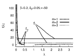
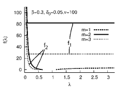
Figure 3: The function $f(\lambda,\ m)$ for $\beta=0.3$, $\delta_{0}=0.05$ and $\beta_{1}=1/4$ in the unaligned logarithmic case with $\beta_{1}=1/4$. In the lower two panels, the two branches of $f_{1}$ and $f_{2}$ with $f_{1}>f_{2}$ are shown for each $m\geq 2$ (see Appendix B). Note that for small $\lambda$, $f_{1}$ and $f_{2}$ branches do not cross each other, although they appear to be extremely close.

For small $\nu$, at least one stationary solution exists for each $m>0$. However for increasing $\nu$ towards the tight-winding regime, stationary perturbation solutions of $m=1$ are shifted towards weaker magnetic fields. For $\nu=50$, solutions for $m=1$ are found within the range $\lambda\approx(1.1,3.25)$ and for $\nu=100$, they are within $\lambda\approx(1.2,3.25)$. Meanwhile, stationary perturbation solutions for $m\geq 2$ grow into a larger range of $\lambda$. If $\nu$ is increased further (i.e. towards the extremely tight-winding regime), two stationary perturbation solutions exist corresponding to each $m$. Thus according to expression (63) for the two roots of $f$, $f_{1}$ and $f_{2}$ are the upper and lower curves in Figure 3, respectively. In the range of $\lambda$ for stationary perturbation solutions, $f_{1}$ remains more or less constant so that a change of magnetic field strength appears independent of the amount of dark matter. Meanwhile, $f_{2}$ changes over a larger range of $\lambda$, indicating that the magnetic field and $f_{2}$ relate each other more closely. The magnetic field is directly connected to $\lambda$. If $f_{1}$ remains constant for all $\lambda$, then the reverse direction of reasoning cannot be used, i.e., for a given $f_{1}=19$ and $\nu=50$, the exact value of $\lambda$ and so $B_{z}$ cannot be determined with certainty. In contrast to $f_{1}$, $f_{2}$ varies for $\nu=50$ over a larger range of $\lambda=(0.1,0.5)$. In this range of $\lambda$, one can determine for each $f_{2}$ the associated $\lambda$ and thus $B_{z}$ through $B_{z}=2\pi\sqrt{G}\Sigma^{g}_{0}/\lambda$. The tighter the spiral arms are wound, the more dark matter is needed in order to maintain stationary logarithmic spiral patterns. This is a general trend of variation and is valid for both roots of $f$. Nevertheless, there exists a certain $\nu_{0}$ value such that the second solution $f_{2}$ appears with a much less amount of dark matter for $\nu>\nu_{0}$. In other words, with increasing $\nu$ the dark matter amount also increases, except for the second solution with $\nu>\nu_{0}$. Physically, the two roots $f_{1}$ and $f_{2}$ are equally valid. But compared with the observational value of $f\approx 10$ for typical spiral galaxies, $f_{1}$ appears too large, e.g. for $\nu=50$ and $f_{1}\approx 19$ within the range of $\lambda=(0.2,\ 3.25)$. In comparison, the lower $f_{2}$ appears more plausible because of its smaller values instead of the very large values of $f_{1}$. For $\nu=100$, one can again find a relation between the $f_{2}$ curve and the magnetic field (represented by $\lambda$) and it is thus also possible to determine $B_{z}$ through the $f$ ratio. If the curve $f_{2}(\lambda)$ is sufficiently steep, so that a one-to-one relation is present between $f_{2}$ and $\lambda$, then the magnetic field strength $B_{z}$ can be determined by integral (18) into

$$B_{z}=\frac{2\pi\sqrt{G}\Sigma^{g}_{0}}{\lambda}\ .$$ (65)

The only additional variable that one needs to know is the surface mass density of the magnetized gas disc. In this paper, we have not explored situations of $\nu\neq 0$ and $\beta_{1}\neq 1/4$ for which both parameters $M$ and $Y_{m}(\beta_{1}-i\nu/2)$ are complex. In this case, an additional study is needed to explore the variation of $\beta_{1}$ and its influence on the gravitational potential ratio $f$. Physically, $\beta_{1}$ is the constant scale-free index of surface mass density perturbations. A larger $\beta_{1}$ corresponds to a steeper radial profile of stationary coplanar perturbations in magnitudes.

9 Model Results for Two Limiting Cases

In the first limit of large $\lambda$ regime (i.e. $B_{z}\rightarrow 0$), we readily reproduce the model results of Shen & Lou (2004) where the gravitational coupling of two scale-free stellar and gaseous discs in the absence of magnetic field is analyzed.

Figure 4: The limiting case of no magnetic field is approximately realized by setting a large isopedic parameter $\lambda=24$.

For the absence of magnetic field, we choose a sufficiently large isopedic parameter $\lambda=24$. The dependence of ratio $f$ on various parameters is shown in Figure 4. For the choice of $\delta_{0}=0.05$ and $\nu=0$, only the case of $m=1$ has stationary perturbation solutions. The variation of $\delta_{0}$ enables $m\geq 2$ to have stationary perturbation configurations as already mentioned in Section 7. For $\nu=0$, each $m$ corresponds to only one stationary perturbation solution. When $\nu$ is sufficiently small, only $m=1$ perturbation configurations have stationary solutions. As $\nu$ is gradually increased, one can see clearly in Fig. 4 panel c) that stationary perturbation solutions for $m\geq 2$ also appear.

In the second limit of large $\delta_{0}$ (i.e. $\Sigma_{0}^{(s)}\rightarrow 0$) for young galaxies in the early Universe, we recover the results of Lou & Wu (2005) where global MHD perturbation configurations in a single isopedically magnetized gaseous disc are studied. Figure 5 shows different variations of $f$ ratio for the aligned and unaligned logarithmic cases in that regime.

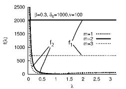
Figure 5: The limiting case of only one single isopedically magnetized gaseous disc is approximately achieved by setting $\delta_{0}=1000$. Two branches $f_{1}$ and $f_{2}$ roots are shown with $f_{1}>f_{2}$ for each $m\geq 2$ (see Appendix B). While they appear very close, $f_{1}$ curve does not intersect $f_{2}$ curve at small $\lambda$.

In principle, all $m$ values can have corresponding stationary solutions for global perturbation configurations. This depends on the choice of $\lambda$ and the combination of different parameters such as $k^{(s)}$, $k^{(g)}$ or $S^{(g)}$ and so forth. For $m=1$, the starting point of stationary solutions for the aligned case is $\lambda\approx 1.1$ and for the unaligned case it is slightly shifted to $\lambda\approx 1.2$. For $m=1$ the range of ratio $f=(0.01,\ 0.5)$ is very small for $\nu=0$ as compared to range $f=(1,\ 60)$ for $\nu=100$. For $m\geq 2$, a variation of $\beta$ parameter in the range of $\beta=(0.1,\ 0.49)$ for the background composite disc configuration does not affect features of $f(\lambda)$ curves very much. In the model of Wu & Lou (2006), potential ratio $f$ is studied for different properties of the magnetized gaseous disc alone (such as the sound speed) at a certain specified value of $\lambda$ parameter. The special case of one single magnetized gaseous disc in our model is complementary to their analysis. Again, the basic fact that typically $f\;\lower 4.0pt\hbox{${\buildrel\displaystyle<\over{\sim}}$}\;10$ must be kept in mind for applications to spiral galaxies. Due to their smaller values for $\nu=100$, the minus-sign solution $f_{2}$ is regarded as more plausible.

10 Conclusions and Discussion

We have investigated global stationary solutions for aligned and unaligned logarithmic perturbation configurations with a constant radial flux of angular momentum and paid special attention to the roles of dark matter halo represented by the $f$ parameter for the gravitational potential ratio and the isopedic parameter $\lambda$. For this purpose, the stationary dispersion relation for global perturbations is derived and a quadratic equation of $f$ is obtained. In our model formulation, the stationary assumption is applied as a very special limiting case of the QSSS hypothesis (e.g. Bertin & Lin 1996 and references therein) which itself is already a very strong requirement to the disc dynamics. For a non-vanishing small pattern speed of a few $\mathrm{km\ s^{-1}kpc^{-1}}$ (adopted in the QSSS theory), a similar relation between $f$ and $B_{z}$ may be also derived. Our sample calculations show that there are three possibilities for potential ratio $f$, corresponding to no solution, one solution and two solutions, respectively. In general, potential ratio $f$ is a fairly complicated function of several independent model parameters involved. In order to explore the dependence of potential ratio $f$ upon $\beta$, $\delta_{0}$, $\lambda$, $m$ and $\nu$, we have chosen typical values for these relevant parameters to characterize late-type disc galaxies. Therefore, these results should be applicable to typical spiral galaxies for comparison. The main results are now summarized below.

10.1 Global Aligned Perturbation Configurations with $\nu=0$ and $\beta_{1}=\beta$

Global aligned perturbation configurations with $\nu=0$ are studied for typical late-type galaxies with different $\beta$ values, corresponding to various power-law radial fall-offs of the disc rotation curve. Examples of our numerical exploration show that in the estimated range of $\lambda$ for disc galaxies, a variation of $\beta$ parameter has no significant impact on global stationary perturbation configurations with $m\geq 1$. As a general trend, a stronger magnetic field allows existence of stationary perturbation configurations for $m\geq 2$. For weaker magnetic fields, only stationary perturbation configurations with $m=1$ (i.e. lopsided cases) may exist. We have also explored stationary perturbation configurations for a disc galaxy at different epochs of evolution by varying the disc surface mass density ratio $\delta_{0}=\Sigma^{(g)}_{0}/\Sigma^{(s)}_{0}$. By our sample calculations, the variation of $\delta_{0}$ strongly affects the behaviour of $f(\lambda)$. This is a consequence of the fact that the magnetic field directly affects the gaseous disc and in an earlier stage of galaxy evolution, the gas fraction is higher in a composite disc system. With increasing $\delta_{0}$ ratio towards earlier epochs ( i.e. at higher cosmological redshifts in the early Universe), the range of allowed stationary perturbation configurations for $m\geq 2$ also increases while that for $m=1$ shrinks. In our simple scenario, $\delta_{0}$ parameter marks the evolution of a disc galaxy in the expanding Universe. At the beginning, a proto-spiral galaxy is presumably composed of a nebulous gas disc and a dark matter halo (e.g. Lou & Wu 2005; Wu & Lou 2006). During the evolution of a spiral galaxy, more and more stars are born and die and thus the disc mass ratio $\delta_{0}$ decreases slowly with time. With this scenario in mind, we interpret Figure 2 as follows. At an earlier stage of disc galaxy evolution, stationary solutions of global perturbation configurations with $m\geq 2$ exist over a wider range of $\lambda$. The influence of magnetic fields there is also stronger as the curve $f(\lambda)$ there varies significantly over a larger range of $\lambda$, indicating a wider range for magnetic field strengths.

This brings out an extremely interesting evolutionary perspective for speculations. Observationally, the global star formation rate (SFR) in spiral galaxies is an important indicative parameter to characterize the galactic evolution. Conceptually, if one attempts to relate this SFR with disc instabilities, the application of Toomre’s criterion (Safonov 1960; Toomre 1964) to a stellar disc alone would be insufficient because stars are directly born in the gaseous disc. Following this line of reasoning, one needs at least to explore instabilities in a composite system of stellar and gas discs (e.g. Lou & Fan 1998, 2000 and references therein) in the presence of a massive dark matter halo. The importance of magnetic fields is generally recognized in the dynamics of star-forming cloud cores. Nevertheless, how to specifically relate physical processes of star formation in clouds on much smaller scales and of large-scale disc instabilities remains a challenging problem due to the tremendous differences in scales. In spite of this challenge, we have developed intuitive feelings that regions of high gas density and strong magnetic fields on large scales are expected to be vulnerable or favorable to active star formation processes. Now in a highly simplified dynamic manner, our model analysis brings together several important aspects for this physical consideration, viz. dark matter halo, magnetic field, and higher gas fraction (i.e. larger $\delta_{0}$) in a composite disc system. The initial conditions for forming a proto-galactic disc nebula such as the dark matter halo, gas disc and magnetic field are expected to be statistical with fluctuations. The instability properties of such a magnetized disc system in the presence of a dark matter halo may then grossly determine the global SFR and thus the galactic evolution. In other words, different initial conditions can lead to different kinds of evolutionary tracks. In particular, it is conceivable that the SFR may have highs and lows along galactic evolutionary paths in the expanding Universe. This information would be valuable for understanding the overall cosmological evolution in terms of global SFRs of spiral galaxies.

To compare a late-type spiral galaxy with an early-type spiral galaxy, we emphasize that stationary perturbation solutions for $m\geq 2$ are very different in these galaxies. In a late-type spiral galaxy of $\delta_{0}\sim 0.05$, stationary perturbation configurations of $m\geq 2$ can only exist for strong magnetic fields while in an earlier stage of evolution, such solutions can exist for almost all $\lambda$ values. These results suggest that multiple-armed disc galaxies may be more numerous in the early Universe. It may be possible for disc galaxies to change patterns during the course of their evolution. Conceivably evolving on cosmological timescales, a disc galaxy pattern may alternately become stationary or quasi-stationary as evidenced by the fact of changing $\delta_{0}$ and $\lambda$, e.g. $f$ and $m\geq 2$ are shifted towards smaller $\lambda$ for stationary configurations. This offers a novel perspective to relate global SFRs of disc galaxies and the galactic pattern speed evolution. For example in numerical simulations, one may start from initially stationary perturbation configurations and then explore time-dependent quasi-stationary behaviours as well as nonlinear effects of a composite disc system by adjusting one or several relevant parameters systematically.

10.2 Global Stationary Unaligned Logarithmic Spiral Configurations with $\beta_{1}=1/4$ and $\nu\neq 0$

Parameter $\nu$ characterizing radial variations of coplanar perturbations affects $f$ ratio in many ways. For example, in spiral galaxies with more tightly wound logarithmic spiral arms (i.e. larger $\nu$), more dark matter is needed in the massive halo to sustain stationary perturbation configurations. Furthermore, with increasing $\nu$ towards the WKBJ regime, each $f$ may correspond to multiple stationary configurations. For very small $\nu$ in the opposite limit, only perturbation configurations with $m=1$ have stationary solutions (i.e. lopsided configurations). Stationary perturbations with $m=1$ also have solutions for larger $\nu$, but only in a certain range of $\lambda\approx(1.2,\ 3.25)$. Larger $\nu$ values have one stationary solution for all $m\geq 2$ (see Appendix B), namely the $f_{1}$ root of expression (63). If $\nu$ is increased further, then the second root $f_{2}$ of expression (63) also fulfills all necessary physical requirements on $f$ parameter. Here, $f_{2}$ root is always smaller than $f_{1}$ root and we expect that whenever there are two theoretical solutions possible, then $f_{2}$ tends to be the more realistic root because of its relatively lower values. The limiting case of $\nu\to\infty$ represents tightly wound spiral arms and the well-known WKBJ approximation (Lin & Shu 1964, 1966) should become applicable.

The curve $f_{2}(\lambda)$ shows that there is a one-to-one correspondence between $f_{2}$ root and strong magnetic fields. Therefore, by determining $f_{2}$ ratio through observations (e.g. rotation curves or gravitational lensing effects) and equation (40), the magnetic field strength can also be determined. For weak magnetic fields, root $f_{2}$ does not vary significantly enough and thus, isopedic magnetic field strength $B_{z}$ cannot be sensibly determined as a result of uncertainties in galactic observations.

10.3 Two Limiting Parameter Regimes

The two limiting cases of $\lambda\to\infty$ and $\delta_{0}\to\infty$ have been explored in the previous section. In the limit of $\lambda\to\infty$, magnetic field almost vanishes and one comes back to two gravitationally coupled hydrodynamic disc system with an axisymmetric dark matter halo. For late-type spiral galaxies, only perturbation configurations of $m=1$ lead to stationary aligned solutions with a positive $f$ ratio. For unaligned logarithmic perturbation configurations with $m\geq 2$, the existence of stationary solutions also depends upon the choice of dimensionless ‘radial wavenumber’ $\nu$. For early-type spiral galaxies of higher $\delta_{0}$, global stationary solutions of all $m$ for perturbation configurations can be found. As already noted, this implies the possibility of more numerous multiple-armed spiral galaxies in the early Universe.

For $\delta_{0}\to\infty$ (see Fig. 5 for large $\delta_{0}$), stationary perturbation solutions for $m\geq 2$ can be found for every chosen parameter set. For $m=1$, solutions exist in a certain range of $\lambda$. For example for $\nu=100$ and $\delta_{0}=1000$, the case of $m=1$ has $f$ roots for $\lambda=(1.2,\ 3.25)$ (see the right panel of Fig. 5).

To conclude for $\delta_{0}\to\infty$, for small $\nu$ or $\nu=0$, all $m$ values have one $f$ root. But for larger $\nu$, the case of $m\geq 2$ can have two $f$ roots. This is the same as that of $\delta_{0}=0.05$. The difference lies in the values of $f$. The larger the ‘radial wavenumber’ $\nu$ value is, the larger are the potential ratios $f_{1}$ and $f_{2}$.

For late-type spiral galaxies and unaligned logarithmic cases, a weak magnetic field does not play a significant role as expected. The younger the spiral galaxy is, the more important the role of a magnetic field especially in the regime of stronger magnetic fields. For very strong magnetic fields, it appears that $f$ ratio is more closely connected to the magnetic field and the effect of magnetic fields cannot be ignored. But for weak magnetic fields, $f$ ratio remains more or less constant for all types of spiral galaxies.

Our results can be summarized as follows. First of all, we emphasize that the lopsided global configuration $m=1$ is an exceptional case for which the curve $f(\lambda)$ has a distinctly different shape as compared to those for the cases $m\geq 2$ (see Appendix B). For both aligned and unaligned logarithmic spiral cases with $m\geq 2$, strong magnetic fields (still realistic in spiral galaxies) can bear a significant relation to the dark matter halo in maintaining globally stationary perturbation configurations.

Physically, we conclude that in spiral galaxies with or without radial variations in perturbations, weak magnetic fields do not influence stationary perturbation configurations. But when the magnetic field strength is increased, a globally stationary perturbation configuration would then become non-stationary if the $f$ ratio is not high enough for the increased magnetic field strength. A change of perturbation patterns might be possible during the course of the galaxy evolution. For example, flocculent galaxies might represent the transitional phase for global pattern changes of galaxies. This prediction may be tested by numerical simulations and by deep survey of morphological observations for galaxies in the early Universe.

Our model analysis has shown that the magnetic field needs to be sensibly chosen with other given disc parameters in order to maintain a global perturbation configuration with a stationary pattern in our frame of reference. Therefore, a variation or an adjustment of $B_{z}$ may put a stationary perturbation configuration into a non-stationary one or a non-stationary perturbation configuration into a stationary one because there exists a one-to-one correspondence between the potential ratio $f$ and a sufficiently strong magnetic field $B_{z}$ for globally stationary perturbation configurations. For such a stationary disc balance in general, the potential ratio $f$ can vary in a considerably large range depending on the choice of other relevant parameters in sensible regimes. As expected on intuitive ground, sufficiently weak magnetic fields exert fairly small influence on stationary perturbation configurations in our composite model. The main reason is that the magnetic pressure and tension together are not strong enough as compared with other forces which play important dynamic roles in our composite system.

In the regime of weak magnetic fields, there also exist instabilities widely explored in the literature. The magneto-Jeans instability (MJI) is an instability which is based on background in-plane magnetic fields. In recent years, several authors (e.g. Kim & Ostriker 2001; Kim, Ostriker & Stone 2002; Shetty & Ostriker 2006) have performed numerical MHD simulations for galaxies. In particular, they studied azimuthal magnetic fields that lie in the disc plane (see also Lou & Zou 2004, 2006; Lou & Bai 2006). For our study of isopedic magnetic fields, as already mentioned, Lou & Wu (2005) have proved that a constant $\lambda$ is a consequence of the frozen-in condition on magnetic flux (see also Wu & Lou 2006). Our composite MHD model offers a two-dimensional description of an isopedic magnetic field. Due to the idealization of razor-thin discs, perturbations lie in the galactic plane and have no $\hat{z}-$components. Hence, a treatment of the magnetorotational instability (MRI) is impossible due to its necessary requirement of a perturbation $e^{ik_{z}z}$ along $\hat{z}-$direction (Chandrasekhar 1960; Balbus & Hawley 1991, 1998; Balbus 2003). When switching over to discs of finite thicknesses, the MRI must be included and a larger $f$ is probably needed in order to counteract MRIs. With our theory, the range of strong vertical magnetic fields is well studied, whereas the effect of weak magnetic fields is underestimated since we do not account for MRIs which play an important role for weak magnetic fields. The results that we obtain here cannot be directly applied to coplanar magnetic fields, thus we can make no predictions for the MJIs.

The galactic application of our disc model results leads to two methods which may be utilised to determine either the isopedic magnetic field strength $B_{z}$ or the mass of an axisymmetric dark matter halo. First, by using equation (40) through observations of a disc galaxy, one can estimate the gravitational potential ratio $f$. In the case of a stationary pattern of a perturbation configuration, only one distribution of magnetic field strengths is possible for this $f$ value. This is a new approach of determining the distribution of isopedic magnetic field strengths in disc galaxies. Proceeding in the opposite direction, these model results may also be applied to determine $f$ ratio by using observationally inferred distribution of magnetic field strengths. This appears to be an alternative method to estimate the halo mass of dark matter. The real challenge of these procedures is to determine whether a perturbation pattern is stationary or quasi-stationary through independent observational diagnostics. In practice, the relevant parameters that need to be determined by galactic observations for our proposed method to work are $m$, $\beta$ (the scaling index for radial variations of unperturbed disc variables), $\beta_{1}^{d}$ (the scaling index for radial variations of perturbation disc variables), unperturbed disc surface mass densities $\Sigma^{(i)}_{0}(r)$, effective sound speeds $a^{(i)}$, either $\lambda$ (for the determination of gravitational potential ratio $f$) or the other way around $f$ (for the determination of distribution of magnetic field strengths $B_{z}$). It is indeed a challenging task for observations to specifically identify some of these parameters and as far as we know, galactic observations so far still have not determined completely all these parameters with error bars in one galaxy.

In addition, this work can also be understood as a preparation for the following study on MHD density waves in such a composite disc system since all relevant quantities and their relations among each other are presented in this work. In reference to singular isothermal disc (SID) models of Shu & Li (1997), Shu et al. (2000), Lou & Shen (2003), Lou & Zou (2004, 2006), Shen et al. (2005), there exist two classes of solutions for stationary magnetohydrodynamic (MHD) perturbation configurations with in-phase and out-of-phase density perturbations in the two discs. We expect for the case of a scale-free stellar disc and an isopedically magnetized scale-free gaseous disc embedded in an axisymmetric dark matter halo, that there are also two classes of in-phase and out-of-phase density perturbations. The formulae and results obtained here can be used later to analyze such MHD density waves.

Appendix A Derivations of stationary dispersion relation and relevant equations

For coplanar MHD perturbations in a background rotating axisymmetric disc system with $v^{(i)}_{r}=v^{(i)}_{r0}+v^{(i)}_{r1}$ , $\ v^{(i)}_{\theta}=v^{(i)}_{\theta 0}+v^{(i)}_{\theta 1}$ , $\ \Sigma^{(i)}=\Sigma^{(i)}_{0}+\Sigma^{(i)}_{1}$ , $\ \Phi^{(i)}=\Phi^{(i)}_{0}+\Phi^{(i)}_{1}$ and $\ H^{(i)}=H^{(i)}_{0}+H^{(i)}_{1}$ in equations $(\ref{eq:conti})-(\ref{eq:euler2})$, where superscript $i$ within parentheses can be set as $s$ and $g$ for stellar and magnetized gaseous discs respectively, it is straightforward to obtain linearized perturbation equations below

$$\frac{\partial\Sigma^{(i)}_{1}}{\partial t}+\frac{1}{r}\frac{\partial}{\partial r}\left[r\Sigma^{(i)}_{0}v^{(i)}_{r1}\right]+\frac{1}{r}\frac{\partial}{\partial\theta}\left[\Sigma^{(i)}_{0}v^{(i)}_{\theta 1}+\Sigma^{(i)}_{1}v^{(i)}_{\theta 0}\right]=0\ ,$$ (66)

$$\frac{\partial v^{(s)}_{r1}}{\partial t}+\Omega^{(s)}_{0}\frac{\partial v^{(s)}_{r1}}{\partial\theta}-2\Omega^{(s)}_{0}v^{(s)}_{\theta 1}=-\frac{\partial\left[H^{(s)}_{1}+\Phi^{(s)}_{1}+\Phi^{(g)}_{1}\right]}{\partial r}\ ,$$ (67)

$$\frac{\partial v^{(g)}_{r1}}{\partial t}+\Omega^{(g)}_{0}\frac{\partial v^{(g)}_{r1}}{\partial\theta}-2\Omega^{(g)}_{0}v^{(g)}_{\theta 1}=-\frac{\partial\left[\Theta H^{(g)}_{1}+\Phi^{(s)}_{1}+\epsilon\Phi^{(g)}_{1}\right]}{\partial r}\ ,$$ (68)

$$\frac{\partial v^{(s)}_{\theta 1}}{\partial t}+v^{(s)}_{r1}\bigg{[}\Omega^{(s)}_{0}+r\frac{\mathrm{d}\Omega^{(s)}_{0}}{\mathrm{d}r}\bigg{]}+\Omega^{(s)}_{0}\frac{\partial v^{(s)}_{\theta 1}}{\partial\theta}+\Omega^{(s)}_{0}v^{(s)}_{r1}=-\frac{\partial\left[H^{(s)}_{1}+\Phi^{(s)}_{1}+\Phi^{(g)}_{1}\right]}{r\partial\theta}\ ,$$ (69)

$$\frac{\partial v^{(g)}_{\theta 1}}{\partial t}+v^{(g)}_{r1}\bigg{[}\Omega^{(g)}_{0}+r\frac{\mathrm{d}\Omega^{(g)}_{0}}{\mathrm{d}r}\bigg{]}+\Omega^{(g)}_{0}\frac{\partial v^{(g)}_{\theta 1}}{\partial\theta}+\Omega^{(g)}_{0}v^{(g)}_{r1}=-\frac{\partial\left[\Theta H^{(g)}_{1}+\Phi^{(s)}_{1}+\epsilon\Phi^{(g)}_{1}\right]}{r\partial\theta}\ ,$$ (70)

where $v^{(i)}_{r0}=0$ for the background disc configuration. Equation (66) represents the two mass conservation equations, equations (67) and (68) are the two radial momentum equations, and equations (69) and (70) are the two azimuthal momentum equations; effects of the isopedic magnetic field are subsumed in the two parameters $\Theta$ and $\epsilon$ (see equations 22 and 23) for the magnetized gaseous disc in momentum equations (68) and (70); and the gravitational coupling between the stellar and gaseous discs is represented by the sum of gravitational potential perturbations $\Phi^{(s)}_{1}+\Phi^{(g)}_{1}$ or $\Phi^{(s)}_{1}+\epsilon\Phi^{(g)}_{1}$ in two-dimensional perturbation equations (67) to (70). As the axisymmetric gravitational potential of a massive dark matter halo is presumed to be unperturbed for simplicity, its perturbation does not appear on the right-hand sides of equations (67) to (70). For perturbations cast in the form of Fourier decomposition, we write for example

$$v^{(i)}_{r1}=A^{(i)}(r)\exp[i(\omega t-m\theta)]\ ,$$ (71)

$$v^{(i)}_{\theta 1}=B^{(i)}(r)\exp[i(\omega t-m\theta)]\ ,$$ (72)

where $m$ is an integral number to characterize azimuthal variations, $\omega$ is the angular perturbation frequency, $A^{(i)}(r)$ and $B^{(i)}(r)$ are small-magnitude functions of radius $r$, and superscripts $i=s,\ g$ stand for associations with stellar and gaseous discs, respectively. Two new frequency parameters are now introduced below for simplicity. The first one is the abbreviation $\overline{\omega}^{(i)}\equiv\omega-m\Omega^{(i)}_{0}$ and the second one is the so-called epicyclic frequency $\kappa^{(i)}_{0}$ of a rotating disc defined by

$$\left[\kappa^{(i)}_{0}\right]^{2}=r\mathrm{d}\left[\Omega^{(i)}_{0}\right]^{2}/\mathrm{d}r+4\left[\Omega^{(i)}_{0}\right]^{2}=2\left[b^{(i)}_{0}\right]^{2}(1-\beta)r^{-2\beta-2}=2(1-\beta)\left[\Omega^{(i)}_{0}\right]^{2}\ .$$ (73)

Substituting all expressions of Fourier harmonics into equations (66)$-$(70), we readily obtain the following perturbation equations

$$\Sigma^{(i)}_{1}i\overline{\omega}^{(i)}+\frac{1}{r}\frac{\partial}{\partial r}\left[r\Sigma^{(i)}_{0}v^{(i)}_{r1}\right]-\frac{im}{r}\Sigma^{(i)}_{0}v^{(i)}_{\theta 1}=0\ ,$$ (74)

$$v^{(s)}_{r1}i\overline{\omega}^{(s)}-2\Omega^{(s)}_{0}v^{(s)}_{\theta 1}=-\frac{\partial\left[H^{(s)}_{1}+\Phi^{(s)}_{1}+\Phi^{(g)}_{1}\right]}{\partial r}\ ,$$ (75)

$$v^{(g)}_{r,1}i\overline{\omega}^{(g)}-2\Omega^{(g)}_{0}v^{(g)}_{\theta 1}=-\frac{\partial\left[\Theta H^{(g)}_{1}+\Phi^{(s)}_{1}+\epsilon\Phi^{(g)}_{1}\right]}{\partial r}\ ,$$ (76)

$$v^{(s)}_{\theta 1}i\overline{\omega}^{(s)}+v^{(s)}_{r1}\frac{\left[\kappa^{(s)}_{0}\right]^{2}}{2\Omega^{(s)}_{0}}=\frac{im\left[H^{(s)}_{1}+\Phi^{(s)}_{1}+\Phi^{(g)}_{1}\right]}{r}\ ,$$ (77)

$$v^{(g)}_{\theta 1}i\overline{\omega}^{(g)}+v^{(g)}_{r1}\frac{\left[\kappa^{(g)}_{0}\right]^{2}}{2\Omega^{(g)}_{0}}=\frac{im\left[\Theta H^{(g)}_{1}+\Phi^{(s)}_{1}+\epsilon\Phi^{(g)}_{1}\right]}{r}\ ,$$ (78)

for both stellar and isopedically magnetized gaseous discs coupled by gravity. Furthermore, the perturbation of surface mass density is set to the following form of Fourier harmonics

$$\Sigma^{(i)}_{1}=S^{(i)}_{1}r^{-2\beta_{1}-1}\exp[i(\omega t-m\theta+\nu\ln r)]=S^{(i)}_{1}r^{-2\beta^{d}_{1}-1}\exp[i(\omega t-m\theta)]\$$ (79)

with $S^{(i)}_{1}$ being small-magnitude coefficients to justify the perturbation approach and

$$\beta^{d}_{1}\equiv\beta_{1}-i\nu/2\$$ (80)

being complex in general for $\nu\neq 0$. The unit complex factor $\exp(-im\theta)$ represents periodic azimuthal variations and the unit complex factor $\exp(i\nu\ln r)$ represents radial variations with $\nu$ closely related to the radial wavenumber. In general, $\beta_{1}$ parameter for perturbations can be different from $\beta$ parameter used for characterizing the background axisymmetric equilibrium disc in rotation. According to several formulae derived by Qian (1992), the corresponding perturbation of gravitational potential associated with a surface mass density perturbation is simply given by

$$\Phi_{1}^{(i)}=-GY_{m}(\beta^{d}_{1})S^{(i)}_{1}r^{-2\beta^{d}_{1}}\exp[i(\omega t-m\theta)]=-GrY_{m}(\beta^{d}_{1})\Sigma^{(i)}_{1}$$ (81)

analytically and the corresponding perturbation of enthalpy is given by

$$H^{(i)}_{1}=\frac{\mathrm{d}H^{(i)}_{0}}{\mathrm{d}\Sigma^{(i)}_{0}}\Sigma^{(i)}_{1}=nk^{(i)}\left[\Sigma^{(i)}_{0}\right]^{n-2}\Sigma^{(i)}_{1}=\frac{\left[a^{(i)}\right]^{2}}{\Sigma^{(i)}_{0}}\Sigma^{(i)}_{1}\ .$$ (82)

It follows immediately that

$$H^{(s)}_{1}+\Phi^{(s)}_{1}+\Phi^{(g)}_{1}=Gr\Sigma^{(s)}_{1}K^{(s)}\ ,\hskip 28.45274pt\mathrm{with}\hskip 28.45274ptK^{(s)}\equiv\frac{\left[a^{(s)}\right]^{2}}{Gr\Sigma^{(s)}_{0}}-Y_{m}(\beta_{1}^{d})(1+\delta_{1})\ ;$$ (83)

$$\Theta H^{(g)}_{1}+\Phi^{(s)}_{1}+\epsilon\Phi^{(g)}_{1}=Gr\Sigma^{(g)}_{1}K^{(g)}\ ,\hskip 28.45274pt\mathrm{with}\hskip 28.45274ptK^{(g)}\equiv\frac{\Theta\left[a^{(g)}\right]^{2}}{Gr\Sigma^{(g)}_{0}}-Y_{m}(\beta_{1}^{d})(\epsilon+\delta_{1}^{-1})\ ,$$ (84)

where $\delta_{1}\equiv\Sigma_{1}^{(g)}/\Sigma_{1}^{(s)}$ is a constant ratio for surface mass density perturbations by expression (79), and $K^{(s)}$ and $K^{(g)}$ defined by equations (83) and (84) respectively are two dimensionless constants because $\big{[}a^{(i)}\big{]}^{2}\propto r^{-2\beta}$ and $r\Sigma^{(i)}_{0}\propto r^{-2\beta}$. For coplanar perturbations in the stellar disc in rotation, we then have the following perturbation equations

$$\Sigma^{(s)}_{1}i\overline{\omega}^{(s)}+\frac{1}{r}\frac{\partial}{\partial r}\left[r\Sigma^{(s)}_{0}v^{(s)}_{r1}\right]-\frac{im}{r}\Sigma^{(s)}_{0}v^{(s)}_{\theta 1}=0\ ,$$ (85)

$$v^{(s)}_{r1}i\overline{\omega}^{(s)}-2\Omega^{(s)}_{0}v^{(s)}_{\theta 1}=-GK^{(s)}\frac{\partial}{\partial r}\left[\Sigma^{(s)}_{1}r\right]\ ,$$ (86)

$$v^{(s)}_{\theta 1}i\overline{\omega}^{(s)}+v^{(s)}_{r1}\frac{\left[\kappa^{(s)}_{0}\right]^{2}}{2\Omega^{(s)}_{0}}=imG\Sigma^{(s)}_{1}K^{(s)}\ .$$ (87)

Meanwhile for coplanar MHD perturbations in the isopedically magnetized gaseous disc in rotation, we obtain in parallel

$$\Sigma^{(g)}_{1}i\overline{\omega}^{(g)}+\frac{1}{r}\frac{\partial}{\partial r}\left[r\Sigma^{(g)}_{0}v^{(g)}_{r1}\right]-\frac{im}{r}\Sigma^{(g)}_{0}v^{(g)}_{\theta 1}=0\ ,$$ (88)

$$v^{(g)}_{r1}i\overline{\omega}^{(g)}-2\Omega^{(g)}_{0}v^{(g)}_{\theta 1}=-GK^{(g)}\frac{\partial}{\partial r}\left[\Sigma^{(g)}_{1}r\right]\ ,$$ (89)

$$v^{(g)}_{\theta 1}i\overline{\omega}^{(g)}+v^{(g)}_{r1}\frac{\left[\kappa^{(g)}_{0}\right]^{2}}{2\Omega^{(g)}_{0}}=imG\Sigma^{(g)}_{1}K^{(g)}\ .$$ (90)

¿From equations $(\ref{eq:2stellar})-(\ref{eq:3stellar})$ and $(\ref{eq:2gaseous})-(\ref{eq:3gaseous})$, we directly derive expressions for radial and azimuthal velocity perturbations $v^{(i)}_{r1}$ and $v^{(i)}_{\theta 1}$ as given below.

$$v^{(i)}_{r1}=\frac{iGK^{(i)}}{\big{[}\overline{\omega}^{(i)}\big{]}^{2}-\big{[}\kappa_{0}^{(i)}\big{]}^{2}}\left(-\frac{2m\Omega_{0}^{(i)}}{r}+\overline{\omega}^{(i)}\frac{\partial}{\partial r}\right)\left[\Sigma^{(i)}_{1}r\right]\ ,$$ (91)

$$v^{(i)}_{\theta 1}=\frac{GK^{(i)}}{\big{[}\overline{\omega}^{(i)}\big{]}^{2}-\big{[}\kappa_{0}^{(i)}\big{]}^{2}}\left(\frac{m\overline{\omega}^{(i)}}{r}-\frac{\big{[}\kappa_{0}^{(i)}\big{]}^{2}}{2\Omega_{0}^{(i)}}\frac{\partial}{\partial r}\right)\left[\Sigma^{(i)}_{1}r\right]\ .$$ (92)

Substituting these expressions into the mass conservation equations and using expression (79), we finally arrive at

$$\frac{\overline{\omega}^{(i)}r}{GK^{(i)}\Sigma^{(i)}_{0}}=\frac{\big{[}m^{2}-4(\beta^{d}_{1})^{2}+2\beta^{d}_{1}\big{]}\overline{\omega}^{(i)}-2m\beta\Omega_{0}^{(i)}}{\big{[}\overline{\omega}^{(i)}\big{]}^{2}-\big{[}\kappa_{0}^{(i)}\big{]}^{2}}-\frac{4(\beta+1)\big{[}m\Omega_{0}^{(i)}+\beta^{d}_{1}\overline{\omega}^{(i)}\big{]}\overline{\omega}^{(i)}\omega}{\left[[\overline{\omega}^{(i)}]^{2}-[\kappa_{0}^{(i)}]^{2}\right]^{2}}\equiv Q^{(i)}\$$ (93)

for both stellar and magnetized gaseous discs, respectively, and for defining the corresponding $Q^{(i)}$. A combination of these two equations for perturbations in stellar and gaseous discs leads to the dispersion relation of the gravity coupled disc configuration, namely

$$\left\{\left[a^{(s)}\right]^{2}-G\Sigma^{(s)}_{0}rY_{m}(\beta^{d}_{1})-\overline{\omega}^{(s)}r^{2}/Q^{(s)}\right\}\left\{\Theta\left[a^{(g)}\right]^{2}-\epsilon G\Sigma^{(g)}_{0}rY_{m}(\beta^{d}_{1})-\overline{\omega}^{(g)}r^{2}/Q^{(g)}\right\}=G\Sigma^{(s)}_{0}rY_{m}(\beta^{d}_{1})G\Sigma^{(g)}_{0}rY_{m}(\beta^{d}_{1})\ .$$ (94)

Relation (94) is comprehensive and it contains all useful information about the disc dynamics after a perturbation has arisen there. Depending on the purpose of investigation, one can define different parameter regimes by using this dispersion relation. We study non-axisymmetric stationary perturbations with $m\neq 0$ and $\omega=0$ which can be either aligned configurations or unaligned logarithmic spirals. For the stationary case of $\omega=0$, equation (94) reduces to

$$\left\{\big{[}a^{(s)}\big{]}^{2}-G\Sigma^{(s)}_{0}rY_{m}(\beta^{d}_{1})-\big{[}\Omega_{0}^{(s)}\big{]}^{2}r^{2}\left[\frac{m^{2}-2(1-\beta)}{m^{2}-4(\beta^{d}_{1})^{2}+2\beta^{d}_{1}+2\beta}\right]\right\}\qquad\qquad\qquad\qquad\qquad\qquad\qquad\qquad\qquad\qquad$$

$$\qquad\times\left\{\Theta\big{[}a^{(g)}\big{]}^{2}-\epsilon G\Sigma^{(g)}_{0}rY_{m}(\beta^{d}_{1})-\big{[}\Omega_{0}^{(g)}\big{]}^{2}r^{2}\left[\frac{m^{2}-2(1-\beta)}{m^{2}-4(\beta^{d}_{1})^{2}+2\beta^{d}_{1}+2\beta}\right]\right\}=\left[G\Sigma^{(s)}_{0}rY_{m}(\beta^{d}_{1})\right]\left[G\Sigma^{(g)}_{0}rY_{m}(\beta^{d}_{1})\right]\ ,$$ (95)

where, according to expressions (40) and (41) for the background equilibrium disc system, we have disc angular rotation speeds given by

$$\Omega_{0}^{(s)}\equiv v^{(s)}_{\theta 0}/r\ \hskip 14.22636pt\mathrm{with}\hskip 14.22636pt\left[v^{(s)}_{\theta 0}\right]^{2}=2\beta rGY_{0}(\beta)\left[\Sigma^{(s)}_{0}+\Sigma^{(g)}_{0}\right](1+f)-\left[a^{(s)}\right]^{2}(2\beta+1)\ ,$$ (96)

$$\Omega^{(g)}_{0}\equiv v^{(g)}_{\theta 0}/r\ \hskip 14.22636pt\mathrm{with}\hskip 14.22636pt\left[v^{(g)}_{\theta 0}\right]^{2}=2\beta rGY_{0}(\beta)\left[\big{[}\Sigma^{(s)}_{0}+\Sigma^{(g)}_{0}\big{]}(1+f)-(1-\epsilon)\Sigma^{(g)}_{0}\right]-\Theta\left[a^{(g)}\right]^{2}(2\beta+1)\ .$$ (97)

As the gravitational potential ratio $f$ should be the same in both equations (40) and (41), a relation between $\big{[}v^{(s)}_{\theta 0}\big{]}^{2}$ and $\big{[}v^{(g)}_{\theta 0}\big{]}^{2}$ can therefore be established, namely

$$\big{[}v^{(s)}_{\theta 0}\big{]}^{2}=\big{[}v^{(g)}_{\theta 0}\big{]}^{2}+(2\beta+1)\big{\{}\Theta\big{[}a^{(g)}\big{]}^{2}-\big{[}a^{(s)}\big{]}^{2}\big{\}}+2\beta rGY_{0}(\beta)(1-\epsilon)\Sigma^{(g)}_{0}\ .$$ (98)

Using expressions $v^{(i)}_{\theta 0}=b^{(i)}_{0}r^{-\beta}$ and $\Sigma^{(i)}_{0}=S^{(i)}_{0}r^{-2\beta-1}$ for the background scale-free disc system, equation (98) can be written as

$$\big{[}b^{(s)}_{0}\big{]}^{2}=\big{[}b^{(g)}_{0}\big{]}^{2}+(2\beta+1)\big{\{}\Theta\big{[}a^{(g)}\big{]}^{2}-\big{[}a^{(s)}\big{]}^{2}\big{\}}r^{2\beta}+2\beta GY_{0}(\beta)(1-\epsilon)S^{(g)}_{0}\$$ (99)

without radial dependence. We now introduce the rotational Mach number $D^{(s)}$ for the stellar disc and the rotational magnetosonic Mach number $D^{(g)}$ for the isopedically magnetized gaseous disc, respectively.

$$D^{(s)}\equiv\frac{v^{(s)}_{\theta 0}}{a^{(s)}}=\frac{b^{(s)}_{0}}{a^{(s)}r^{\beta}}\ ,\hskip 28.45274pt\rightarrow\hskip 28.45274ptb^{(s)}_{0}=a^{(s)}r^{\beta}D^{(s)}\ ;$$ (100)

$$D^{(g)}\equiv\frac{v^{(g)}_{\theta 0}}{\sqrt{\Theta}a^{(g)}}=\frac{b^{(g)}_{0}}{\sqrt{\Theta}a^{(g)}r^{\beta}}\ ,\hskip 28.45274pt\rightarrow\hskip 28.45274ptb^{(g)}_{0}=\sqrt{\Theta}a^{(g)}r^{\beta}D^{(g)}\ .$$ (101)

Using background disc equilibrium equations (40), (41) and (99), the following relations can then be derived,

$$\big{[}D^{(s)}\big{]}^{2}=\frac{2\beta GY_{0}(\beta)S^{(s)}_{0}(1+\delta_{0})(1+f)}{\big{[}a^{(s)}\big{]}^{2}r^{2\beta}}-(2\beta+1)\ ,$$ (102)

$$\big{[}D^{(g)}\big{]}^{2}=\frac{2\beta GY_{0}(\beta)S^{(g)}_{0}\big{[}f(1+\delta_{0}^{-1})+\delta^{-1}_{0}+\epsilon\big{]}}{\Theta\big{[}a^{(g)}\big{]}^{2}r^{2\beta}}-(2\beta+1)\ ,$$ (103)

$$\big{[}D^{(s)}\big{]}^{2}=\big{[}D^{(g)}\big{]}^{2}\Delta+(2\beta+1)(\Delta-1)+2\beta GY_{0}(\beta)(1-\epsilon)S^{(g)}_{0}\big{/}\big{[}[a^{(s)}]^{2}r^{2\beta}\big{]}\ ,$$ (104)

with ratio $\Delta\equiv\Theta\big{[}a^{(g)}\big{]}^{2}\big{/}\big{[}a^{(s)}\big{]}^{2}$. With these defined quantities and relations (102), (103) and (104), stationary dispersion relation (95) can be cast into

$$\left\{1-\frac{GS^{(s)}_{0}Y_{m}(\beta^{d}_{1})}{\big{[}a^{(s)}\big{]}^{2}r^{2\beta}}-\left[D^{(s)}\right]^{2}\left[\frac{m^{2}-2(1-\beta)}{m^{2}-4(\beta^{d}_{1})^{2}+2\beta^{d}_{1}+2\beta}\right]\right\}\qquad\qquad\qquad\qquad\qquad\qquad\qquad\qquad$$

$$\times\left\{1-\frac{\epsilon GS^{(g)}_{0}Y_{m}(\beta^{d}_{1})}{\Theta\big{[}a^{(g)}\big{]}^{2}r^{2\beta}}-\left[D^{(g)}\right]^{2}\left[\frac{m^{2}-2(1-\beta)}{m^{2}-4(\beta^{d}_{1})^{2}+2\beta^{d}_{1}+2\beta}\right]\right\}=\frac{GS^{(s)}_{0}Y_{m}(\beta^{d}_{1})}{\big{[}a^{(s)}\big{]}^{2}r^{2\beta}}\frac{GS^{(g)}_{0}Y_{m}(\beta^{d}_{1})}{\Theta\big{[}a^{(g)}\big{]}^{2}r^{2\beta}}\ .$$ (105)

A.1 Two Cases of Real Stationary Dispersion Relation and Relevant Mathematical Expressions

Our main purpose is to establish relations between dark matter halo (represented by $f$ ratio) and an isopedic magnetic field in gaseous disc (represented by the isopedic ratio $\lambda$). For the two cases of $\beta_{1}^{d}=\beta_{1}=\beta$ (with $\nu=0$) and of $\beta_{1}=1/4$ (with $\nu\neq 0$), we show in the following that $M$ and $Y_{m}$ as defined by equations (53) and (35) become real numbers. In the literature, $\beta_{1}^{d}=\beta$ is called the aligned case since the radial wavenumber parameter $\nu$ vanishes in this case and thus, only azimuthal and no radial wave variations are present. In this case, we have

$$M=\frac{m^{2}-2(1-\beta)}{m^{2}+4\beta(1-\beta)}\ ,\qquad\qquad\qquad\qquad\quad\ \$$ (106)

$$Y_{m}(\beta)=\frac{\pi\Gamma(m/2-\beta+1/2)\Gamma(m/2+\beta)}{\Gamma(m/2-\beta+1)\Gamma(m/2+\beta+1/2)}\ .$$ (107)

For $\nu\neq 0$ and thus a complex $\beta_{1}^{d}$, the general expressions for $M$ and $Y_{m}(\beta_{1}^{d})$ are

$$M=\frac{m^{2}-2(1-\beta)}{m^{2}+2(\beta+\beta_{1}-2\beta_{1}^{2}+\nu^{2}/2)+i\nu(4\beta_{1}-1)}\ ,\qquad\qquad\quad$$ (108)

$$Y_{m}(\beta_{1}^{d})=\frac{\pi\Gamma(m/2-\beta_{1}+i\nu/2+1/2)\Gamma(m/2+\beta_{1}-i\nu/2)}{\Gamma(m/2-\beta_{1}+i\nu/2+1)\Gamma(m/2+\beta_{1}-i\nu/2+1/2)}\ .$$ (109)

By setting $\beta_{1}=1/4$ in expressions (108) and (109), we immediately have

$$M=\frac{m^{2}-2(1-\beta)}{m^{2}+2\beta+1/4+\nu^{2}}\ ,\qquad\qquad$$ (110)

$$Y_{m}(\beta_{1}^{d})=\left|\frac{\Gamma(m/2+1/4+i\nu/2)}{\Gamma(m/2+3/4+i\nu/2)}\right|^{2}\ .$$ (111)

Expression (111) is based on the relation $\Gamma(z)^{*}=\Gamma(z^{*})$ for Gamma-function where ^∗ denotes the complex conjugate operation. For these two cases $\beta_{1}^{d}=\beta_{1}=\beta$ (with $\nu=0$) and of $\beta_{1}=1/4$ (with $\nu\neq 0$ in general), we explore numerically the behaviour $f(\lambda)$ by specifying other relevant model parameters.

Appendix B Dependence of gravity potential ratio $f$ on perturbation orders $m$

Here, we briefly describe the gravitational potential ratio $f$ as a function for different $m$ values and provide an upper limit for the difference of $f(m+2)-f(m)$. In general, the function $f$ depends on $m$ through functional parameters $M$ and $Y_{m}(\beta_{1}^{d})$. In the limit of $m\to\infty$, we have $M\to 1$ and therefore the difference $\Delta M=M(m+1)-M(m)\to 0$. For the property of functional parameter $Y_{m}(\beta_{1}^{d})$, we first discuss the property of Gamma-function. For Gamma functions, the well-known recursion formula is simply

$$\Gamma(x+1)=x\Gamma(x)\ ,$$ (112)

which immediately leads to the following four relations

$$\Gamma((m+2)/2-\beta_{1}^{d}+1/2)=(m/2-\beta_{1}^{d}+1/2)\Gamma(m/2-\beta_{1}^{d}+1/2)\ ,$$ (113)

$$\Gamma((m+2)/2+\beta_{1}^{d})=(m/2+\beta_{1}^{d})\Gamma(m/2+\beta_{1}^{d})\ ,$$ (114)

$$\Gamma((m+2)/2-\beta_{1}^{d}+1)=(m/2-\beta_{1}^{d}+1)\Gamma(m/2-\beta_{1}^{d}+1)\ ,$$ (115)

$$\Gamma((m+2)/2+\beta_{1}^{d}+1/2)=(m/2+\beta_{1}^{d}+1/2)\Gamma(m/2+\beta_{1}^{d}+1/2)\$$ (116)

as applied to our case under consideration. Therefore, we have

$$Y_{m+2}(\beta^{d}_{1})=\frac{\big{(}m-2\beta_{1}^{d}+1\big{)}\big{(}m+2\beta_{1}^{d}\big{)}}{\big{(}m-2\beta_{1}^{d}+2\big{)}\big{(}m+2\beta_{1}^{d}+1\big{)}}Y_{m}(\beta^{d}_{1})\ .$$ (117)

For $m\to\infty$, it follows that $Y_{m+2}(\beta_{1}^{d})\to Y_{m}(\beta_{1}^{d})$, indicating the difference $\Delta Y_{m}(\beta_{1}^{d})=Y_{m+2}(\beta^{d}_{1})-Y_{m}(\beta_{1}^{d})\to 0$. Based on these analyses, we conclude that for very large values of $m$, there is no significant difference between $f(m+2)$ and $f(m)$, and therefore $f(m+2)\to f(m)$ in the limit of large $m$ values.

For $m=2$, we have from equations (53) and (117)

$$M(4)-M(2)=\frac{7+\beta}{8-2(\beta^{d}_{1})^{2}+\beta^{d}_{1}+\beta}-\frac{1+\beta}{2-2(\beta^{d}_{1})^{2}+\beta^{d}_{1}+\beta}\ ,$$ (118)

$$Y_{4}(\beta^{d}_{1})-Y_{2}(\beta^{d}_{1})=\left[\frac{(3-2\beta_{1}^{d})(1+\beta_{1}^{d})}{(2-\beta_{1}^{d})(3+2\beta_{1}^{d})}-1\right]Y_{2}(\beta^{d}_{1})=\left[\frac{3+\beta_{1}^{d}-2(\beta_{1}^{d})^{2}}{6+\beta_{1}^{d}-2(\beta_{1}^{d})^{2}}-1\right]Y_{2}(\beta^{d}_{1})\equiv NY_{2}(\beta^{d}_{1})\ ,$$ (119)

Figure 6: For the left panel, the difference of $M(4)-M(2)$ is shown as a function of $\beta$ parameter with a fixed real $\beta_{1}^{d}$, with a maximum at $\beta=-0.25$ and $\beta_{1}^{d}\sim 0.25$; for a real value of $\beta_{1}^{d}$, the difference $M(4)-M(2)$ appears to be a monotonically decreasing function with increasing $\beta$ value. For the right panel, the difference of $M(4)-M(2)$ is shown as a function of real $\beta_{1}^{d}$ values with a fixed value $\beta=-0.25$. A maximum value can be readily identified.

which defines the coefficient $N$ as a function of $\beta^{d}_{1}$ that is complex for $\nu\neq 0$. The difference $M(4)-M(2)$ is a function of both $\beta$ and $\beta^{d}_{1}$. The largest difference is found for $\beta=-0.25$ and $\beta_{1}^{d}\sim 0.2-0.3$ with $\Delta M\equiv M(4)-M(2)=0.46$ (see Figure 6). For applications to spiral galaxies, only positive $\beta$ values are physically relevant. But for a theoretical consideration, a negative $\beta$ is allowed to estimate limit. To conclude, we obtain

$$\Delta M\leq 0.46\ .$$ (120)

Figure 7: Variation of coefficient $N(\beta_{1}^{d})$ defined by equation (119) as a function of real $\beta_{1}^{d}$ values. The factor $N(\beta_{1}^{d})$ in relation $Y_{4}=(N+1)Y_{2}$ as a function of $\beta_{1}^{d}$.

For a real range of $\beta_{1}^{d}\in[-0.5,0.5]$ with $\nu=0$, functional parameter $N(\beta_{1}^{d})$ is plotted in Figure 7. The smallest $N$ is $-0.6$ for $\beta_{1}^{d}=-0.5$. From equation (117), one can also see that $Y_{m+2}(\beta^{d}_{1})$ is always smaller than $Y_{m}(\beta^{d}_{1})$. This fact explains the negative values shown in Figure 7. For the absolute difference, we get inequality

$$|\Delta Y_{m}|=|Y_{m+2}-Y_{m}|\leq 0.6Y_{m}\ .$$ (121)

In contrast to $\Delta M$ which can be determined as a constant, $\Delta Y_{m}$ is a function of $Y_{m}$. For $\Delta f$, the upper limit is $f(4)-f(2)$ which is different each time depending on the chosen parameters. As a result, the difference of two functions $f(n)$ and $f(n+2)$ with $n=m,m+1,\cdots$ goes towards zero, namely

$$f(m+2)-f(m)\to 0\hskip 28.45274pt\mathrm{for}\hskip 28.45274ptm\to\infty\ .$$ (122)

$$f(m+3)-f(m+1)\to 0\hskip 28.45274pt\mathrm{for}\hskip 28.45274ptm\to\infty\ .$$ (123)

Appendix C Perturbation density ratio $\delta_{1}$ in the model disc system

In order to compare the mass density perturbations in the two discs, the ratio $\delta_{1}=\Sigma_{1}^{(g)}/\Sigma_{1}^{(s)}$ is derived in the following by using equation (93). This ratio $\delta_{1}$ is contained implicitly in $K^{(i)}$ expressions. Using this relation for the stellar disc and $\omega^{(g)}=0$, we derive

$$\delta_{1}=\frac{\Sigma^{(g)}_{1}}{\Sigma^{(s)}_{1}}=\frac{-\big{[}D^{(s)}\big{]}^{2}\big{[}A^{(s)}\big{]}^{2}\big{[}m^{2}-2(1-\beta)\big{]}}{GS^{(s)}_{0}Y_{m}(\beta^{d}_{1})\big{[}m^{2}-4(\beta^{d}_{1})^{2}+2\beta^{d}_{1}+2\beta\big{]}}+\frac{\big{[}A^{(s)}\big{]}^{2}}{GS^{(s)}_{0}Y_{m}(\beta^{d}_{1})}-1\ .$$ (124)

We substitute expression (104) of $D^{(s)}$ into equation (124) to relate the two discs. With $N=-(m^{2}-2+2\beta)\ ,$ we then obtain

$$\delta_{1}=N\frac{(D^{(g)})^{2}\Theta(A^{(g)})^{2}+(2\beta+1)\big{[}\Theta(A^{(g)})^{2}-(A^{(s)})^{2}\big{]}+2\beta GY_{0}(\beta)(1-\epsilon)S^{(g)}_{0}}{GY_{m}(\beta_{1}^{d})S^{(s)}_{0}\big{[}m^{2}-4(\beta^{d}_{1})^{2}+2\beta^{d}_{1}+2\beta\big{]}}+\frac{(A^{(s)})^{2}}{GS^{(s)}_{0}Y_{m}(\beta_{1}^{d})}-1\ .$$ (125)

The ratio $\delta_{1}=\Sigma^{(g)}_{1}/\Sigma^{(s)}_{1}$ is negative in the case of out-of-phase density wave perturbations. For this case, the gravity effect is weaker and the MHD density wave speed is faster. In the case of in-phase density wave perturbations, this ratio $\delta_{1}$ is positive, the gravity effect is stronger and the MHD density wave speed is slower (Lou & Fan 1998).

References

- (1) Balbus S. A., 2003, ARA&A, 41, 555
- (2) Balbus S. A., Hawley J. F., 1991, ApJ, 376, 214
- (3) Balbus S. A., Hawley J. F., 1998, Rev. Mod. Phys., 70, 1
- (4) Baldwin J. E., Lynden-Bell D., Sancisi R., 1980, MNRAS, 193, 313
- (5) Beck R., Brandenburg A., Moss D., Shukorov A., Sokoloff D., 1996, ARA&A, 34, 155
- (6) Bertin G., Lin C. C., 1996, Spiral Structure in Galaxies. MIT Press, Cambridge, MA
- (7) Bertin G., Lin C. C., Lowe S. A., Thurstans R. P., 1989a, ApJ, 338, 78
- (8) Bertin G., Lin C. C., Lowe S. A., Thurstans R. P., 1989b, ApJ, 338, 104
- (9) Binney J., Tremaine S., 1987, Galactic Dynamics. Princeton Univ. Press, Princeton
- (10) Bosma A., 1981, AJ, 86, 1825B
- (11) Brown J. C., Taylor A. R., Wielebinski R., Mueller P., 2003, ApJ, 592, L29
- (12) Chakrabarti S., Laughlin G., Shu F. H., 2003, ApJ, 596, 220
- (13) Chakrabarti S., 2008, submitted (astro-ph/08120821)
- (14) Chandrasekhar S., 1961, Hydrodynamic and Hydromagnetic Instability. Clarendon, Oxford University
- (15) Diemand J., Kuhlen M., Madau P., Zemp M., Moore B., Potter D., Stadel J., 2008, Nature, 454, 735
- (16) Gittins D. M., Clarke C. J., 2004, MNRAS, 349, 909
- (17) Goldreich P., Tremaine S., 1979, ApJ, 233, 857
- (18) Kendall S., Kennicutt R. C., Clarke C., Thornley M. D., 2008, MNRAS, 387, 1007
- (19) Kent S. M., 1986, AJ, 91, 1301
- (20) Kent S. M., 1987, AJ, 93, 816
- (21) Kent S. M., 1988, AJ, 96, 514
- (22) Kim W., Ostriker E. C., 2001, ApJ, 559, 70
- (23) Kim W., Ostriker E. C., Stone J. M., 2002, ApJ, 581, 1080
- (24) Krumm N., Salpeter E. E., 1976, ApJ, 208, L7
- (25) Krumm N., Salpeter E. E., 1977, A&A, 56, 465
- (26) Landau L. D., Lifshitz E. M., 1959, Fluid Mechanics. Pergamon, Oxford
- (27) Li Z.-Y., Shu F. H., 1996, ApJ, 468, 261
- (28) Lin C. C., Shu F. H., 1964, ApJ, 140, 646
- (29) Lin C. C., Shu F. H., 1966, Proc. Nat. Acad. Sci., 55, 229
- (30) Lizano S., Shu F. H., 1989, ApJ, 342, 834
- (31) Lou Y.-Q., Bai X. N., 2006, MNRAS, 372, 81
- (32) Lou Y.-Q., Fan Z. H., 1998, MNRAS, 297, 84
- (33) Lou Y.-Q., Fan Z. H., 2000, MNRAS, 315, 646
- (34) Lou Y.-Q., Shen Y., 2003, MNRAS, 343, 750
- (35) Lou Y.-Q., Wu Y., 2005, MNRAS, 364, 475
- (36) Lou Y.-Q., Zou Y., 2004, MNRAS, 350, 1220
- (37) Lou Y.-Q., Zou Y., 2006, MNRAS, 366, 1037
- (38) Lynden-Bell D., Lemos J. P. S., 1999 (astro-ph/9907093)
- (39) Nakano T., 1979, PASJ, 31, 697
- (40) Ostriker J. P., Peebles P. J. E., 1973, ApJ, 186, 467
- (41) Ostriker J. P., Peebles P. J. E., Yahil A., 1974, ApJ, 193, L1
- (42) Qian E., 1992, MNRAS, 257, 581
- (43) Roberts M. S., 1962, AJ, 67, 437
- (44) Roberts M. S., Rots A. H., 1973, A&A, 26, 483
- (45) Rubin V. C., 1965, ApJ, 142, 934
- (46) Safronov V. S., 1960, Ann. d’Astrophys., 23, 979
- (47) Shen Y., Liu X., Lou Y.-Q., 2005, MNRAS, 356, 1333
- (48) Shen Y., Lou Y.-Q., 2003, MNRAS, 345, 1340
- (49) Shen Y., Lou Y.-Q., 2004, MNRAS, 353, 249
- (50) Shetty R., Ostriker E. C., 2006, ApJ, 647, 997
- (51) Shu F.-H., Laughlin G., Lizano S., Galli D., ApJ, 2000, 535, 190
- (52) Shu F.-H., Li Z.-Y., 1997, ApJ, 475, 251
- (53) Sofue Y., Fujimoto M., Wielebinski R., 1986, ARA&A, 24, 459
- (54) Syer D., Tremaine S., 1996, MNRAS, 281, 925
- (55) Toomre A., 1964, ApJ, 139, 1217
- (56) Toomre A., 1977, ARA&A, 15, 437
- (57) Visser H. C. D., 1980a, A&A, 88, 149
- (58) Visser H. C. D., 1980b, A&A, 88, 159
- (59) Wentzel D. D., 1963, A&A, 1, 195
- (60) Wu Y., Lou Y.-Q., 2006, MNRAS, 372, 992
- (61) Zhang S. J., Jin J. M., 1996, Computation of Special Functions. John Wiley & Sons, New York
- (62) Zweibel E. G., Heiles C., 1997, Nature, 385, 131