Soliton localization in Bose-Einstein condensates with time-dependent harmonic potential and scattering length

Abstract

We derive exact solitonic solutions of a class of Gross-Pitaevskii equations with time-dependent harmonic trapping potential and interatomic interaction. We find families of exact single-solitonic, multi-solitonic, and solitary wave solutions. We show that, with the special case of an oscillating trapping potential and interatomic interaction, a soliton can be localized indefinitely at an arbitrary position. The localization is shown to be experimentally possible for sufficiently long time even with only an oscillating trapping potential and a constant interatomic interaction.

I Introduction

The experimental realization of solitons in Bose-Einstein condensates burger ; denschlag ; anderson ; randy ; schreck ; eirman has stimulated intense interest in their properties perez1 ; busch ; linear1 ; cast ; linear2 ; kasa ; sala0 ; abdu ; sala . The inhomogeneity provided by the trapping potential has renewed the old zab ; has0 ; chen ; konotop1 ; franco and more recent serk interest in the different aspects of one- and multi-solitons dynamics in inhomogeneous potentials.

In the experiments of Refs. randy ; schreck , stable bright solitons were created and set in a particle-like center-of-mass motion. The wave nature of solitons was revealed when two adjacent solitons repelled each other as a result of their phase difference linear1 . On the other hand, it is established that bright solitons collapse when the number of atoms exceeds a certain limit book . This results from the attractive Hartree energy overcoming the repulsive kinetic energy pressure. One of the methods proposed to stabilize the soliton against collapsing is to rapidly oscillate the interatomic interaction or the trapping potential vibrating . Obviously, the inhomogeneity imposed by the trapping potential plays an important role on the dynamics and stability of solitons.

The evolution of solitons is approximately described by the inhomogeneous nonlinear Schr$\ddot{\rm o}$dinger equation known as the Gross-Pitaeviskii equation gpref1 ; gpref2 . The approximation stems from the fact that the Gross-Pitaevskii equation is a mean-field approximation of the exact $N$-particle Schr$\ddot{\rm o}$dinger equation. While in some cases the soliton dynamics obtained by these two equations disagree castan , the Gross-Pitaevskii equation often gives accurate results. Theoretical studies performed to account for the observed behavior of solitons were conducted by solving the Gross-Pitaevskii equation with numerical, perturbative, or variational methods. Much less effort was devoted to finding exact solutions of this equation chen ; wu ; ieee ; jun ; liang ; lu ; raj ; usamapre ; ramesh . In addition to providing rigorous insight, exact solutions acquire valuable importance when problems such as soliton-soliton collisions and soliton interaction with potentials are addressed. In such cases, formulae for the force between solitons or soliton’s effective mass can be derived gordon . In addition, obtaining such exact solutions allows for testing the validity of the Gross-Pitaevskii equation at high soliton densities and obtaining the long-time evolution of the soliton where numerical techniques aught to break down.

Here, we further explore exact solitonic solutions of the Gross-Pitaevskii equation. Specifically, the goal of this paper is two-fold. First, we investigate the existence and properties of solitonic solutions in the presence of time-dependent trapping potential and interatomic interaction. Secondly, we focus on the effect of an oscillating trapping potential and interatomic interaction on the center-of-mass motion of the soliton. We consider here only the case of attractive interatomic interactions which allows for bright solitons.

The first goal is achieved by employing the Darboux transformation method salle to derive families of exact solitonic solutions of a class of Gross-Pitaevskii equations. It should be noted that the main solution we derive here (Eq. (22)), which corresponds to a harmonic expulsive potential, reproduces a special case of the general solution found by Serkin et al. corresponding to a combination of a harmonic and linear potentials serk . Hence, the significance of the first goal is mainly presenting a systematic method of generating exact solutions.

For the second goal, we considered the special case of oscillating strengths of the harmonic trapping potential and interatomic interaction. Interestingly enough, it turns out that such oscillations not only stabilize the soliton against shrinking, but also make it possible to localize it at an arbitrary position. This is the main result of this paper. The possibility of localizing the soliton is then discussed from an experimental point of view. To that end, we considered the nonintegrable, though experimentally simpler, case of only an oscillating trapping potential and constant interatomic interaction. Here too, the soliton can be localized, though not indefinitely as before. The long-time evolution shows that the soliton continues to be trapped but will be oscillating around the minimum of the harmonic potential. For a typical experimental setup, we show that the soliton can be localized around its initial position for a time period of the order of, or even larger than, the lifetime of the soliton. The soliton localization suggests a management mechanism for the soliton position and speed that may have applications in various situations such as soliton-soliton collisions and soliton interaction with potentials.

The rest of the paper is organized as follows. In the next section, we present the general form of the Gross-Pitaevskii equation to be solved. In section III, we use the Darboux transformation method to derive the new solitonic solutions. We then discuss their properties, dynamics, and localization. In section IV, we discuss the experimental feasibility of realizing soliton localization. We end in section V with a summary of our main results and conclusions.

II The Gross-Pitaevskii equation

The Gross-Pitaevskii equation describing a Bose-Einstein condensate trapped by an axially-symmetric harmonic potential with attractive interatomic interactions is given by

$$i\hbar{\partial\over\partial t}\psi({\bf r},t)=\left[-{\hbar^{2}\over 2m}\nabla_{\bf r}^{2}+{1\over 2}m\,\left(\omega_{x}^{2}\,x^{2}+\omega_{\perp}^{2}(y^{2}+z^{2})\right)-{4\,\pi\,a_{s}\,\hbar^{2}\over m}|\psi({\bf r},t)|^{2}\right]\psi({\bf r},t),$$ (1)

where $a_{s}$ is the absolute value of the $s$-wave scattering length, and $\omega_{x}$ and $\omega_{\perp}$ are the characteristic frequencies of the harmonic trapping potential in the axial and radial directions, respectively.

When the confinement of the Bose-Einstein condensate is much larger in the $y$ and $z$ directions compared to the confinement in the $x$ direction, the system can be considered effectively one-dimensional along the $x$ direction. The three-dimensional Gross-Pitaevskii equation can then be integrated over the $y$ and $z$ directions to result in a one-dimensional Gross-Pitaevskii equation perez1 ; carr

$$i\hbar{\partial\over\partial t}\psi(x,t)=\left[-{\hbar^{2}\over 2m}{\partial^{2}\over\partial x^{2}}+{1\over 2}m\,\omega_{x}^{2}\,x^{2}-2\lambda\,a_{s}|\psi(x,t)|^{2}\right]\psi(x,t),$$ (2)

where $\lambda=\omega_{\perp}/\omega_{x}$. Scaling length to $a_{x}=\sqrt{\hbar/m\omega_{x}}$, time to $1/\omega_{x}$, and $\psi(x,t)$ to $1/\sqrt{2\lambda\,a_{x}}$, the Gross-Pitaevskii equation takes the dimensionless form

$$i{\partial\over\partial t}\psi(x,t)=\left[-{1\over 2}{\partial^{2}\over\partial x^{2}}+{1\over 2}\,p(t)\,x^{2}-a\,q(t)|\psi(x,t)|^{2}\right]\psi(x,t),$$ (3)

where $a=a_{s}/a_{x}$ is the scaled scattering length. The dimensionless general functions $p(t)$ and $q(t)$ are introduced to account for the time-dependencies of the strengths of the trapping potential and the interatomic interaction.

In the subsequent section, it is shown that this equation is integrable only if $p(t)$ and $q(t)$ are parametrically related as follows: $p(t)={\ddot{\gamma}}(t)-{\dot{\gamma}}(t)^{2}$ and $q(t)=\exp{(\gamma(t))}$, where $\gamma(t)$ is an arbitrary real function (see Eq. (7)). We find exact solitonic solutions of Eq. (3) below in terms of the function $\gamma(t)$. A host of rich and interesting physical systems are described by such a class of solutions. In particular, an oscillating form of $\gamma(t)$ will be considered in this paper.

III Darboux Transformation and the Exact Solutions

III.1 Darboux Transformation

Applying the Darboux transformation method on nonlinear partial differential equations requires finding a linear system of equations for an auxiliary field ${\bf\Psi}(x,t)$. The linear system is usually written in a compact form in terms of a pair of matrices as follows: ${\bf\Psi}_{x}={\bf U}\cdot{\bf\Psi}$ and ${\bf\Psi}_{t}={\bf V}\cdot{\bf\Psi}$. The matrices ${\bf U}$ and ${\bf V}$, known as the Lax pair, are functionals of the solution of the differential equation. The consistency condition of the linear system ${\bf\Psi}_{xt}={\bf\Psi}_{tx}$ is required to be equivalent to the partial differential equation under consideration. Applying the Darboux transformation, as defined below, on ${\bf\Psi}$ transforms it into another field ${\bf\Psi}[1]$. For the transformed field ${\bf\Psi}[1]$ to be a solution of the linear system, the Lax pair must also be transformed in a certain manner. The transformed Lax pair will be a functional of a new solution of the same differential equation.

Practically, this is performed as follows. First, we find the Lax pair and an exact solution of the differential equation, known as the seed solution. Fortunately, the trivial solution can be used as a seed, leading to nontrivial solutions. Using the Lax pair and the seed solution, the linear system is then solved and the components of ${\bf\Psi}$ are found. The new solution is expressed in terms of these components and the seed solution. The following detailed derivation of the new solution clarifies this procedure further.

Using our Lax Pair search method usama_darboux , we find the following linear system which corresponds to the class of Gross-Pitaevskii equations we are interested in:

$${\bf\Psi}_{x}=\zeta{\bf J\cdot\Psi\cdot\Lambda}+{\bf U\cdot\Psi},$$ (4)

$${\bf\Psi}_{t}=i\zeta^{2}{\bf J\cdot\Psi\cdot\Lambda\cdot\Lambda}+\zeta\,\left(i{\bf U}+x\,\gamma(t)\,{\bf J}\right){\bf\cdot\Psi\cdot\Lambda}+{\bf V\cdot\Psi},$$ (5)

where,

${\bf\Psi}(x,t)=\left(\begin{array}[]{cc}\psi_{1}(x,t)&\psi_{2}(x,t)\\ \phi_{1}(x,t)&\phi_{2}(x,t)\end{array}\right)$,     ${\bf J}=\left(\begin{array}[]{cc}1&0\\ 0&-1\end{array}\right)$,     $\\ \\ \\ {\bf\Lambda}=\left(\begin{array}[]{cc}\lambda_{1}&0\\ 0&\lambda_{2}\end{array}\right)$,     ${\bf U}=\left(\begin{array}[]{cc}0&\sqrt{a}Q(x,t)\\ -\sqrt{a}Q^{*}(x,t)&0\end{array}\right)$,


${\bf V}=\left(\begin{array}[]{cc}ia|Q(x,t)|^{2}/2&\sqrt{a}\lambda x{\dot{\gamma}}Q(x,t)+i\sqrt{a}Q_{x}(x,t)/2\\ -\sqrt{a}\lambda x{\dot{\gamma}}Q^{*}(x,t)+i\sqrt{a}Q^{*}_{x}(x,t)/2&-ia|Q(x,t)|^{2}/2\end{array}\right)$,


$\zeta(t)=\exp{\left(\gamma(t)\right)}$, and $\lambda_{1}$ and $\lambda_{2}$ are arbitrary constants. For convenience, we presented the matrices in terms of the function $Q(x,t)$ which is related to the wave function as follows $Q(x,t)=\psi(x,t)e^{(\gamma(t)+i{\dot{\gamma}}(t)x^{2})/2}$.

It should be emphasized that while applying the Darboux transformation is almost straightforward, finding a linear system that corresponds to the differential equation at hand is certainly not a trivial matter. Usually, this is found by trial and error, or by starting from a certain linear system and then finding the differential equation it corresponds to. In Ref. usama_darboux , we have introduced a systematic approach to find the linear system which we describe here briefly. The partial derivatives of the auxiliary field, ${\bf\Psi}_{x}$ and ${\bf\Psi}_{t}$, are expanded in powers of $\bf\Lambda$ with unknown matrix coefficients. The expansions are terminated at the first order for ${\bf\Psi}_{x}$ and the second order for ${\bf\Psi}_{t}$ since this will be sufficient to generate the class of Gross-Pitaevskii equations under consideration. The higher order matrix coefficients turn out to be essentially determined by the zeroth order matrix coefficients $\bf U$ and $\bf V$. To find the matrices $\bf U$ and $\bf V$, we expand them in powers of the wavefunction $\psi(x,t)$, its complex conjugate, and their partial derivatives. The coefficients of the expansions are unknown functions of $x$ and $t$. Substituting these expansions in the consistency condition (Eq. (6) below) we find a set of equations for the unknown function coefficients. Finally, by solving these equations the Lax pair and consequently the linear system will be determined. The linear system found here is a generalization to that of Zakharov-Shabat for homogeneous Gross-Pitaevskii equation zs .

For ${\bf\Psi}$ to be a solution of both Eqs. (4) and (5), the consistency condition ${\bf\Psi}_{xt}={\bf\Psi}_{tx}$ must be satisfied. This condition leads to the following relation between the matrices $\bf U$ and $\bf V$

$${\bf U}_{t}-{\bf V}_{x}+[{\bf U},{\bf V}]=0,$$ (6)

where $[{\bf U},{\bf V}]$ is the commutator of ${\bf U}$ and ${\bf V}$. Substituting the above expressions for $\bf U$ and $\bf V$ in the last equation, we obtain the Gross-Pitaevskii equation

$$i{\partial\over\partial t}\psi(x,t)=\left[-{1\over 2}{\partial^{2}\over\partial x^{2}}+{1\over 2}\left({\ddot{\gamma}}(t)-{\dot{\gamma}}(t)^{2}\right)x^{2}\psi(x,t)-a\,e^{{\gamma(t)}}|\psi(x,t)|^{2}\right]\psi(x,t),$$ (7)

and its complex conjugate. This equation shows that the functions $p(t)$ and $q(t)$ are parametrically related to each other through the general function $\gamma(t)$. In Ref. serk , Serkin et al. solve a nonautonomous Gross-Pitaevskii equation that is similar to Eq. (7) but with additional time-dependent dispersion and linear potential. Similar to our conclusion usama_darboux , the authors of this reference and Ref. ramesh found that relations between the coefficients must be obeyed for the the model to be integrable. We focus here on the specific case of only a harmonic trapping potential and constant dispersion. The linear system of 8 equations, Eqs. (4) and (5), read explicitly

$$\psi_{1x}-\phi_{1}\sqrt{a}\,e^{\frac{1}{2}\left(i\dot{\gamma}x^{2}+\gamma\right)}\psi_{0}-\sqrt{2}\lambda_{1}\psi_{1}e^{\gamma}=0,$$ (8)

$$\psi_{2x}-\phi_{2}\sqrt{a}\,e^{\frac{1}{2}\left(i\dot{\gamma}x^{2}+\gamma\right)}\psi_{0}-\sqrt{2}\lambda_{2}\psi_{2}e^{\gamma}=0,$$ (9)

$$\phi_{1x}+\sqrt{2}\lambda_{1}\,e^{\gamma}\phi_{1}+\psi_{0}^{*}\psi_{1}\sqrt{a}\,e^{\frac{1}{2}\left(\gamma-ix^{2}\dot{\gamma}\right)}=0,$$ (10)

$$\phi_{2x}+\sqrt{2}\lambda_{2}\,e^{\gamma}\phi_{2}+\psi_{0}^{*}\psi_{2}\sqrt{a}\,e^{\frac{1}{2}\left(\gamma-ix^{2}\dot{\gamma}\right)}=0,$$ (11)

$$\psi_{1t}-i\psi_{1}e^{\gamma}\left(2e^{\gamma}\lambda_{1}^{2}-i\sqrt{2}x\dot{\gamma}\lambda_{1}+{1\over 2}\left|\psi_{0}\left|{}^{2}\right.\right.a\right)-{1\over 2}\phi_{1}\sqrt{a}\,e^{\frac{1}{2}\left(i\dot{\gamma}x^{2}+\gamma\right)}\left(i\psi_{0x}+\psi_{0}\left(2i\sqrt{2}e^{\gamma}\lambda_{1}+x\dot{\gamma}\right)\right)=0,$$ (12)

$$\psi_{2t}-i\psi_{2}e^{\gamma}\left(2e^{\gamma}\lambda_{2}^{2}-i\sqrt{2}x\dot{\gamma}\lambda_{2}+{1\over 2}\left|\psi_{0}\left|{}^{2}\right.\right.a\right)-{1\over 2}\phi_{2}\sqrt{a}\,e^{\frac{1}{2}\left(i\dot{\gamma}x^{2}+\gamma\right)}\left(i\psi_{0x}+\psi_{0}\left(2i\sqrt{2}e^{\gamma}\lambda_{2}+x\dot{\gamma}\right)\right)=0,$$ (13)

$$\phi_{1t}+{1\over 2}\psi_{1}\sqrt{a}\,e^{\frac{1}{2}\left(\gamma-ix^{2}\dot{\gamma}\right)}\left(\psi_{0}^{*}\left(2i\sqrt{2}e^{\gamma}\lambda_{1}+x\dot{\gamma}\right)-i\psi_{0x}^{*}\right)+{1\over 2}\phi_{1}e^{\gamma}\left(i\left|\psi_{0}\left|{}^{2}\right.\right.a+2\lambda_{1}\left(2ie^{\gamma}\lambda_{1}+\sqrt{2}x\dot{\gamma}\right)\right)=0,$$ (14)

$$\phi_{2t}+{1\over 2}\psi_{2}\sqrt{a}\,e^{\frac{1}{2}\left(\gamma-ix^{2}\dot{\gamma}\right)}\left(\psi_{0}^{*}\left(2i\sqrt{2}e^{\gamma}\lambda_{2}+x\dot{\gamma}\right)-i\psi_{0x}^{*}\right)+{1\over 2}\phi_{2}e^{\gamma}\left(i\left|\psi_{0}\left|{}^{2}\right.\right.a+2\lambda_{2}\left(2ie^{\gamma}\lambda_{2}+\sqrt{2}x\dot{\gamma}\right)\right)=0,$$ (15)

where $\psi_{0}(x,t)$ is an exact seed solution of Eq. (7). These equations reduce to an equivalent system of 4 equations with nontrivial solutions by making the following substitutions: $\lambda_{1}=-\lambda_{2}^{*}$, $\psi_{2}=\phi_{1}^{*}$, and $\phi_{2}=-\psi_{1}^{*}$. Using the trivial solution, $\psi_{0}(x,t)=0$, as a seed, the linear system will have the solution

$$\psi_{1}(x,t) = {c_{1}}e^{2i\lambda_{1}^{2}\int e^{2\gamma(t)}\,dt+e^{\gamma(t)}{\lambda_{1}}x},$$ (16)

$$\phi_{2}(x,t) = {c_{2}}e^{-2i\lambda_{1}^{2}\int e^{2\gamma(t)}\,dt-e^{\gamma(t)}{\lambda_{1}}x},$$ (17)

where $c_{1}$ and $c_{2}$ are real arbitrary constants of integration.

Consider the following version of the Darboux transformation salle

$${\bf\Psi}[1]={\bf\Psi}\cdot{\bf\Lambda}-\sigma{\bf\Psi},$$ (18)

where ${\bf\Psi}[1]$ is the transformed field, $\sigma={{\bf\Psi_{0}}}\cdot{\bf\Lambda}\cdot{\bf\Psi_{0}}^{-1}$. Here $\bf\Psi_{0}$ is a known (seed) solution of the linear system Eqs. (8-15). For the transformed field ${\bf\Psi}[1]$ to be a solution of the linear system, the matrix $\bf U$ for instance must be transformed as note

$${\bf U}[1]=\sigma\cdot{\bf U}\cdot\sigma^{-1}+\sigma_{x}\cdot\sigma^{-1},$$ (19)

where $\sigma^{-1}$ is the inverse of $\sigma$. This equation gives the new solution in terms of the seed solutions of the Gross-Pitaevskii equation, $\psi_{0}(x,t)$, and the linear system, ${\bf\Psi_{0}}$, which reads

$$\psi(x,t)=\psi_{0}(x,t)+{2\over a}(\lambda_{1}+\lambda_{1}^{*})e^{-i{\dot{\gamma}}(t)x^{2}/4+\gamma(t)/2}{\phi_{1}\psi_{1}^{*}\over|\phi_{1}|^{2}+|\psi_{1}|^{2}}.$$ (20)

III.2 Exact single-solitonic solution

Using $\psi_{0}(x,t)=0$ and Eqs. (16) and (17), the new solution takes the form

$$\psi(x,t)=\frac{4\sqrt{2}\,{\lambda_{1r}}\,{c_{1}}\,{{{c_{2}}}^{*}}}{{\sqrt{{a}}}}\frac{e^{\gamma(t)/2+i\theta(t)}}{|c_{1}|^{2}e^{\beta(t)x-x_{0}(t)}+|c_{2}|^{2}e^{-(\beta(t)x-x_{0}(t))}},$$ (21)

where $\theta(t)=-4\,\left({{\lambda_{1i}}}^{2}-{{\lambda_{1r}}}^{2}\right)\,\int e^{2\,\gamma(t)}\,dt{+x\,\left(2\,e^{\,\gamma(t)}\,{\lambda_{1i}}-x\,{\dot{\gamma}}(t)/\sqrt{8}\right)}$, $\beta(t)=2\sqrt{2}{\lambda_{1r}}\,e^{\gamma(t)}$, and $x_{0}(t)=8\,{\lambda_{1i}}\,{\lambda_{1r}}\,\int e^{2\,\gamma(t)}\,dt$. Here $c_{1}$, $c_{2}$, $\lambda_{1}$, and $\lambda_{2}$ are arbitrary constants. The subscripts $r$ and $i$ denote real and imaginary parts, respectively. Substituting $c_{1}=\exp{(\delta_{1})}$, $c_{2}=\exp{(\delta_{2})}$, where $\delta_{1}$ and $\delta_{2}$ are arbitrary constants, completing the square in the phase factor, and normalizing $\psi(z,t)$ to $N$, this solution can be recast in the following more appealing form

$$\psi(x,t)={\sqrt{N}\sqrt{N\,a}\over 2}\,e^{\gamma(t)/2+i\phi(x,t)}{\rm sech}{\left({N\,a\over 2}\,e^{\gamma(t)}(x-x_{\rm cm}(t))\right)},$$ (22)

where

$$\phi(x,t)=\phi_{0}(t)+{\dot{x}_{\rm cm}}(t)\,(x-x_{\rm cm}(t))-{1\over 2}{\dot{\gamma}}(t)(x-x_{\rm cm}(t))^{2},$$ (23)

$$x_{\rm cm}(t)=\left(x_{0}e^{2\gamma(0)}+\left(v_{0}+x_{0}\,{\dot{\gamma}}(0)\right)g(t)\right)e^{-\gamma(t)-\gamma(0)},$$ (24)

$$\phi_{0}=c_{3}-{1\over 2}{\dot{\gamma}}(t)^{2}\,x_{\rm cm}(t)^{2}+{1\over 2}\left({1\over 4}({a\,N})^{2}+e^{-2\gamma(0)}\left(v_{0}+x_{0}\,{\dot{\gamma}}(0)\right)^{2}\right)g(t),$$ (25)

$g(t)=\int_{0}^{t}e^{2\gamma(t^{\prime})}dt^{\prime}$. The constant $c_{3}$ corresponds to an arbitrary overall phase.

This solution corresponds to a sech-shaped soliton containing $N$ atoms with a time-dependent center-of-mass $x_{\rm cm}(t)$ and time-dependent width $2\exp(-\gamma\,t)/N\,a$. The linear part of the phase profile shows that the soliton is moving with a center-of-mass velocity $v(t)={\dot{x}}_{\rm cm}(t)$. The quadratic part corresponds to a phase chirp associated with the quadratic trapping potential.

The simple choice $\gamma(t)=constant$, which corresponds to the homogeneous Gross-Pitaevskii equation, gives $x_{\rm cm}(t)=v_{0}\,t+x_{0}$. The solitonic solution in this case corresponds to the well-known sech-shaped soliton with a center-of-mass moving with a constant velocity $v_{0}$ and starting the motion at the initial position $x_{0}$. In the limit $\gamma(t)\rightarrow 0$, the solution, Eq. (22), reduces to

$$\psi(x,t)={\sqrt{N}\sqrt{N\,a}\over 2}\,e^{i\,\phi(t)}{\rm sech}{\left({N\,a\over 2}(x-(x_{0}+v_{0}\,t))\right)},$$ (26)

where $\phi(t)=c_{3}+((a\,N)^{2}+4v_{0}^{2})\,t/8+v_{0}\left(x-(x_{0}+v_{0}\,t)\right)$. This is the well-known sech solution of the homogeneous Gross-Pitaevskii equation. For $\gamma(t)=constant\times t$ we get a Gross-Pitaevskii equation with an expulsive harmonic potential and exponentially growing interatomic interaction liang . In principle, we can choose any form of $\gamma(t)$, but one should keep in mind that the interatomic interaction strength is proportional to $\exp{(\gamma(t))}$. Such a time-dependence may not be realistic from an experimental point of view for any $\gamma(t)$.

In Ref. serk Serkin et al. have already derived the exact solitonic solution of a Gross-Pitaevskii equation with a linear and quadratic potentials and time-dependent dispersion

$$i{\partial\over\partial t}\psi(x,t)=\left[-{D(t)\over 2}{\partial^{2}\over\partial x^{2}}-{\Omega^{2}(t)\over 2}x^{2}-2\alpha(t)x-a\,R(t)|\psi(x,t)|^{2}\right]\psi(x,t).$$ (27)

The authors show that this equation is integrable only if the functions $D(t)$, $\Omega(t)$ and $R(t)$ are related to each other through the integrability condition (Eq. (2) in Ref. serk ). The special case of only a quadratic potential and constant dispersion corresponds to the Gross-Pitaevskii equation considered in this paper. Substituting $\alpha(t)=0$ and $D(t)=1$ in Eq. (2) of Ref. serk , the integrability condition simplifies to $\Omega^{2}=-{\dot{\gamma}}^{2}+{\ddot{\gamma}}$, which shows that, in this special case, the previous equation is indeed equivalent to Eq. (7). Therefore, substituting $\alpha(t)=0$ and $D(t)=1$ in the general solution of Eq. (27), namely Eq. (8) in Ref. serk , should result in our solution, Eq. (22). It turns out, however, that the two solutions do not match exactly. The solution of Ref. serk corresponds to a soliton located initially at $x=0$ while in our case the soliton is located initially at the arbitrary position $x_{0}$. This can be clearly seen by substituting, without loss of generality, $\eta(t)=N\,a\,\exp(\gamma(t))/4$ and $\kappa(t)=-v_{0}\,\exp(-\gamma(0))/2$ in the argument of the sech function of Eq. (8) of Ref. serk . This results in a center of mass coordinate $x_{\rm cm}(t)=v_{0}g(t)\,e^{-\gamma(t)-\gamma(0)}$. Since $g(0)=0$, this shows that $x_{\rm cm}(0)=0$ in contrast with our case $x_{\rm cm}(0)=x_{0}$.

The dynamics of the soliton is readily given by Eq. (24). An equation of motion for the center-of-mass $x_{\rm cm}(t)$ can be derived from the Euler’s equation of the lagrangian $L[x_{\rm cm},{\dot{x}}_{\rm cm}]=\int_{-\infty}^{\infty}i\,dx\,\psi^{*}{\partial\psi/\partial t}-E[x_{\rm cm},{\dot{x}}_{\rm cm}]$. The energy functional is given by

$$E[x_{\rm cm},{\dot{x}}_{\rm cm}]=\int_{-\infty}^{\infty}\psi^{*}(x,t)\left[-{1\over 2}{\partial^{2}\over\partial x^{2}}+{1\over 2}\,({\ddot{\gamma}}(t)-{\dot{\gamma}}(t)^{2})\,x^{2}-{1\over 2}a\,e^{\gamma(t)}|\psi(x,t)|^{2}\right]\psi(x,t),$$ (28)

which results in the equation of motion

$${\ddot{x}}_{\rm cm}(t)+({\ddot{\gamma}}-{\dot{\gamma}}^{2})x_{\rm cm}(t)=0.$$ (29)

This equation shows that the center-of-mass motion is determined by the function $\gamma(t)$. Thus, interatomic interactions do not affect the center-of-mass motion which is a manifestation of Kohn’s theorem kohn .

III.3 Oscillating trapping potential

In this section, we consider an oscillating form of $\gamma(t)$ which results in a trapping potential and interatomic interaction with oscillating strengths. A first simple choice for $\gamma(t)$ would be for instance $\cos{(\omega\,t+\delta)}$. However, in this case, the interatomic interaction, which will be proportional to $\exp{(\cos{\omega\,t+\delta})}$, oscillates nonlinearly. Such time-dependent interatomic interaction may not be possible to realize experimentally. Instead, we use the form

$$\gamma(t)={1\over 2}(\alpha_{1}+\alpha_{2}\cos{(\omega t+\delta)}),$$ (30)

where $\alpha_{1}$, $\alpha_{2}$, $\omega$, and $\delta$ are arbitrary dimensionless constants. In this case, the Gross-Pitaevskii equation, Eq. (7), takes the form

$$i{\partial\psi(x,t)\over\partial t}=\left[-{1\over 2}{\partial^{2}\over\partial x^{2}}-{1\over 4}\alpha_{2}\omega^{2}\left(\cos{(\omega t+\delta)}+{1\over 2}\alpha_{2}\sin{(\omega t+\delta)^{2}}\right)x^{2}-a\,e^{(\alpha_{1}+\alpha_{2}\cos{(\omega t+\delta)})/2}|\psi(x,t)|^{2}\right]\psi(x,t).$$ (31)

The advantage of this particular form of $\gamma(t)$ is that, for $\alpha_{2}\ll 1$, the amplitude of the oscillation in the interatomic interaction can be set to an arbitrarily small value such that the strength of the interatomic interaction can be considered practically as constant. Substituting this expression for $\gamma(t)$ in Eq.(29), we get

$${\ddot{x}}_{\rm cm}-{1\over 4}\alpha_{2}\,\omega^{2}\,\left(2\cos{(\omega\,t+\delta)}+\alpha_{2}\sin{(\omega\,t+\delta)}^{2}\right)x_{\rm cm}=0.$$ (32)

The general solution of this equation is readily given by Eq. (24), which now takes the form

$$x_{\rm cm}(t)=x_{0}\,e^{{\alpha_{2}\over 2}(\cos{\delta}\,-\cos{(\omega\,t+\delta)})}+\left(v_{0}-{1\over 2}x_{0}\,\alpha_{2}\,\omega\,\sin{\delta}\right)e^{-{\alpha_{2}\over 2}(\cos{\delta}+\cos{(\omega\,t+\delta)})}\int_{0}^{t}{dt^{\prime}\,e^{\alpha_{2}\,\cos{(\omega\,t^{\prime}+\delta)}}}.$$ (33)

The first term of this equation corresponds to a bounded oscillation, but the presence of the integral in the second term makes $x_{\rm cm}(t)$ unbounded. Due to this term, the soliton will be expelled out of the trap, i.e., $x_{\rm cm}(t\rightarrow\infty)=\pm\infty$. Therefore, the soliton can be localized, by choosing the parameters such that the prefactor of the unbounded term vanishes, namely

$$v_{0}={1\over 2}x_{0}\,\alpha_{2}\,\omega\,\sin{\delta}.$$ (34)

With this condition, the center-of-mass of the soliton is given by

$$x_{\rm cm}(t)=x_{0}\,e^{{\alpha_{2}\over 2}(\cos{\delta}\,-\cos{(\omega\,t+\delta)})}.$$ (35)

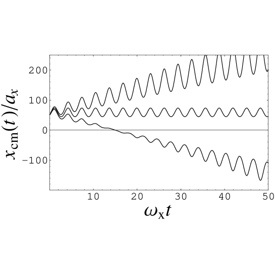
Figure 2: Soliton’s center-of-mass trajectory for three values of the initial velocity. The upper curve corresponds to $v_{0}=1.2\times x_{0}\,\alpha_{2}\omega\,\sin{(\delta)}/2=12.6$, the middle curve corresponds to $v_{0}=x_{0}\,\alpha_{2}\omega\,\sin{(\delta)}/2=10.5$, and the lower curve corresponds to $v_{0}=0.8\times x_{0}\,\alpha_{2}\omega\,\sin{(\delta)}/2=8.4$. For the three curves, we take $\alpha_{1}=1$, $\alpha_{2}=0.5$, $\omega=2$, $\delta=1$, and $x_{0}=50$.

This is one of the main conclusions of this paper. It shows that the soliton can be localized at an arbitrary position by oscillating the strength of the trapping potential and the interatomic interaction. Without such oscillations, the soliton will be expelled out of the trap. In fact, this result also holds for any bounded type of oscillations as can be inferred from Eq. (24). Taking $v_{0}+x_{0}\,{\dot{\gamma}}(0)=0$, this equation gives $x_{\rm cm}(t)=x_{0}\,e^{\gamma(0)-\gamma(t)}$, which is bounded for any bounded $\gamma(t)$. The different cases of soliton localization and delocalization, described by Eq. (33), are shown in Figs. 1 and 2. In Fig. 1, the soliton is shown to be expelled out of the left (right) side of the trap when $v_{0}<x_{0}\,\alpha_{2}\,\omega\,\sin{(\delta)}/2$ ($v_{0}>x_{0}\,\alpha_{2}\,\omega\,\sin{(\delta)}/2$), while for $v_{0}=x_{0}\,\alpha_{2}\,\omega\,\sin{(\delta)}/2$, the soliton remains localized around its initial position $x_{0}$. In Fig. 2, this is shown with the trajectory of the center-of-mass of the soliton.

Notice that in order to localize the soliton, no condition on $\omega$ was required. Therefore, one may argue that by taking $\omega$ arbitrarily small, we get a localized soliton in an almost stationary expulsive harmonic trap. This of course contradicts the fact that in an expulsive harmonic trap, solitons are expelled away from the center. However, one should keep in mind that with our special form of $\gamma(t)$, namely Eq. (30), the strength of the trapping potential will be proportional to $\omega^{2}$. Therefore, a very small value of $\omega$ corresponds to a shallow potential that approaches the homogeneous case for $\omega=0$. The fact that the strength of the harmonic potential depends on $\omega$ leads to conclude that, for deep traps, larger trap oscillations frequency are needed to localize the soliton contrary to the case with shallow traps where the soliton can be localized with smaller trap oscillations frequency.

Taking the time average of the trapping potential $(\omega/2\pi)\int_{0}^{2\pi/\omega}d\,t\,({\ddot{\gamma}}(t)-{\dot{\gamma}}(t)^{2})\,x^{2}/2=-\alpha_{2}^{2}\,\omega^{2}\,x^{2}/16$ shows that the soliton spends on the average more time in the expulsive trapping potential. One may thus conclude that after sufficiently long time the soliton will be expelled out of the trap which contradicts our previous localization result. A careful examination of the dynamics shows that this conclusion is incorrect. In spite of the fact that the soliton spends more time in the expulsive trap, the inhomogeneity of the trapping potential can compensate for the time difference. The strength of the trapping potential has in general two periods $\tau_{1}$ and $\tau_{2}$, as shown in Fig. 3. The period $\tau_{1}$ depends on $\alpha_{2}$ and $\tau_{2}=2\pi/\omega$. The strength of the trapping potential is positive for a period of $\tau_{1}$ and negative for $\tau_{2}-\tau_{1}>\tau_{1}$ for all $\alpha_{2}$. Assuming the soliton started the motion at $x_{0}>0$ from rest, it will experience at first a harmonic trapping potential for time $\tau_{1}$ and therefore will move to the left (region of lower potential) for a certain distance. At time $\tau_{1}$, the trapping potential becomes expulsive for time period $\tau_{2}-\tau_{1}$ and the soliton starts to return back. However, it starts now from a point of lower potential than at $x_{0}$ which means that it will experience a weaker trapping potential. Therefore, in order to reach the starting point, $x_{0}$, it needs more time compared to the forward part of the motion. If that time matches $\tau_{2}-\tau_{1}$, the soliton returns back to $x_{0}$ with zero velocity and the cycle repeats leading to trapping of the soliton, which corresponds to the middle curve of Fig. 2. On the other hand, if the soliton reaches a point $x>x_{0}$, it will be eventually expelled out of the right side of the trap corresponding to the upper curve of Fig. 2, and if it reaches $x<x_{0}$, it will be expelled out of the left side of the trap corresponding to the lower curve of Fig. 2.

To further understand this trapping mechanism, we calculated the trapping potential felt by the soliton through its trajectory, namely $V(x_{\rm cm}(t))$, which is plotted in Fig. 4. In this figure, the dynamics of the soliton is represented by a point moving on the curve with a direction that is indicated on each curve. The center-of-mass motion of Fig. 2 can be extracted by tracing $x_{\rm cm}(t)$ while the point moves along the potential curves. In Fig.4a, the soliton starts at $x_{0}=50$ with initial velocity $v_{0}=1.2\,\alpha_{2}\,x_{0}\,\omega\,\sin{(\delta)}/2$. In this case, the soliton gets drifted by time towards larger values of $x_{\rm cm}$ corresponding to the upper curve of Fig. 1. In Fig. 4c, the initial velocity is $v_{0}=\,\alpha_{2}\,x_{0}\,\omega\,\sin{(\delta)}/2$, which results in soliton localization. In this subfigure, the soliton oscillates between $x_{\rm cm}=50$ and $x_{\rm cm}=61$ corresponding to the middle curve of Fig. 2. In Fig. 4e, the initial velocity is $v_{0}=0.8\,\alpha_{2}\,x_{0}\,\omega\,\sin{(\delta)}/2$ leading to a drift towards lower values of $x_{\rm cm}$ corresponding to the lower curve of Fig. 2. To make an analogy with a classical particle moving in a time-independent potential, we defined $V_{\rm eff}(x_{\rm cm}(t))=V(x_{\rm cm}(t))-[V(x_{\rm cm}(\pi/\omega))-V(x_{\rm cm}(0))][x_{\rm cm}(t)-x_{\rm cm}(0)]/[x_{\rm cm}(\pi/\omega)-x_{\rm cm}(0)]$. In Figs. 4b, d, f, we plot $V_{\rm eff}(x_{\rm cm})$ that corresponds to Figs. 4a, c, e, respectively. The dynamics is now simplified to that of a classical particle oscillating in a ladder of parabolic potentials. For the nonlocalized soliton, the potential minimum is shifted by time to the right (Fig. 4b) or to the left (Fig. 4f). For the localized soliton case, the minimum of the potential is stationary.

III.4 Another family of exact solutions

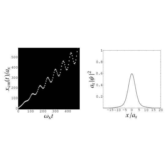
Figure 5: (Left) Spatiotemporal contour plot of soliton density profile. (Right) Soliton density profile at $t=0$. The values of the parameters used in this plot are: $c_{1}=-c_{2}=10$, $c_{3}=c_{4}=1$, $\lambda_{1i}=\lambda_{1r}=1$, $A=2$, $a=0.9$, $k_{0}=5$, $\lambda=\omega=1$, $\delta=0$, $\alpha_{1}=-6$, $\alpha_{2}=0.3$. The value of $k_{0}$ is the solution of $\alpha=0$ with respect to $k_{0}$.

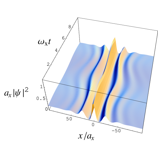
Figure 7: (Color online) Density profile of a single soliton solution. The values of the parameters used in this plot are: $-c_{2}=c_{1}=10$, $c_{3}=c_{4}=1$, $\lambda_{1i}=\lambda_{1r}=1$, $A=2$, $a=0.9$, $k_{0}\sim 5.03$, $\lambda=\omega=1$, $\delta=0$, $\alpha_{1}=-6$, $\alpha_{2}=0.3$. The value of $k_{0}$ is the solution of $\alpha=0$ with respect to $k_{0}$.

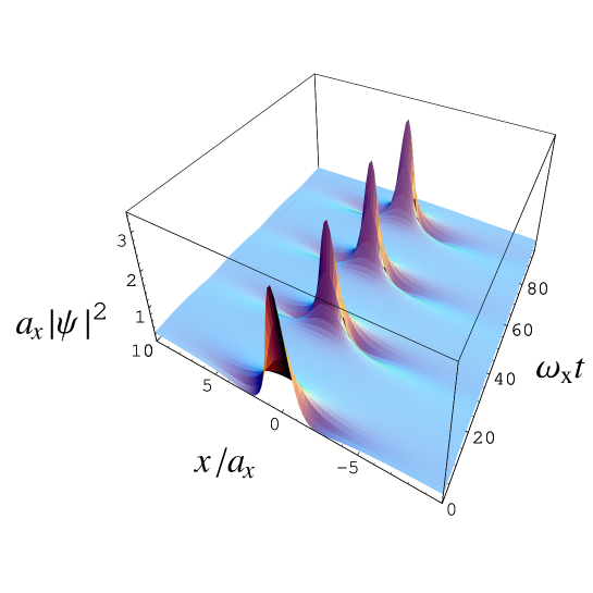
Figure 8: (Color online) Density profile of a multi-solitons solution. The values of the parameters used in this plot are: $-c_{2}=c_{1}=10$, $c_{3}=c_{4}=1$, $\lambda_{1i}=0$, $\lambda_{1r}=1$, $A=2$, $a=0.9$, $k_{0}=0$, $\lambda=1$, $\omega=0.01$, $\delta=0$, $\alpha_{1}=-2$, $\alpha_{2}=0.3$.

Using the exact solution found above as a seed solution, the Darboux transformation generates a two-solitons solution. This kind of solution is useful for studying soliton-soliton interactions which is left for future work. Another family of more complicated exact solitonic solutions can be obtained by using a nontrivial seed solution as shown in Appendix A. Substituting for $\gamma(t)$ in Eq. (41), we get the second class of exact solutions. This family of solutions is more complicated than the above single-solitonic solution since it involves, in addition to the single-solitonic solutions, multi-solitonic and solitary wave solutions. Here, we present briefly the main properties of the solutions of this kind. In Fig. 5, we plot the density of a single-solitonic solution showing that the soliton is being expelled out of the center of the trap. The oscillation in the trajectory of the soliton is due to the oscillating trapping potential. The discontinuous appearing of the soliton is due to the interaction with the background. This trajectory can also be extracted from the general solution, Eq. (41), by considering the term $(\Gamma c_{1}^{2}e^{2\alpha\eta-\sqrt{\dot{\eta}}\Delta_{r}x}+\Gamma c_{2}^{2}e^{-2\alpha\eta+\sqrt{\dot{\eta}}\Delta_{r}x})$ in the denominator. At the soliton’s density peak this is the dominant term that determines the position of the soliton. Specifically, the position of the peak is given by the condition $2\alpha\eta-\sqrt{\dot{\eta}}\Delta_{r}x=0$. Using this condition to plot $x$ versus $t$ in Fig. 6, we obtain a curve that is identical to the soliton trajectory in Fig. 5. The mean slope of this curve is proportional to $\alpha/2\Delta_{r}$. Hence, the rate at which the soliton leaves the center of the trapping potential can be delayed by choosing the parameters and the arbitrary constants such that $\alpha/2\Delta_{r}$ is small. For the special case of $\alpha=0$ the center-of-mass of the soliton will be localized at $x=0$ indefinitely. In this case, the oscillating trapping potential results only in oscillations in the width and peak density of the soliton. This is also shown in Fig. 7 where we see a multi-solitonic solution with central soliton being localized at $x=0$ and off-central ones oscillating around their initial positions. In Fig. 8, we show that for some values of the parameters the dynamics of the peak soliton density can be so drastic such that the soliton disappears in the background and reappears at regular discrete times.

IV Numerical solution and experimental realization

As we have seen in section III.3, there is a possibility to localize the soliton by oscillating the trapping potential and the interatomic interaction in the manner described by Eq. (31). Such synchronized oscillations may not be possible to realize experimentally. Instead, a setup with an oscillating strength of the trapping potential and constant interatomic interaction may be experimentally more favorable. This situation can be obtained in our case with the condition $\alpha_{2}\ll 1$ resulting in the following Gross-Pitaevskii equation

$$i{\partial\psi(x,t)\over\partial t}=\left[-{\partial^{2}\over\partial x^{2}}-{1\over 2}\Omega^{2}\cos{(\omega t+\delta)}\,x^{2}-a\,|\psi(x,t)|^{2}\right]\psi(x,t)$$ (36)

where $\Omega=\omega\,\sqrt{\alpha_{2}/2}$ and we have set $\alpha_{1}=0$. We solve this equation numerically using the exact solution of the homogeneous case, namely the solution of Eq. (36) with $\Omega=0$, as the initial wavefunction. This can be obtained from Eq. (22) simply by substituting $\alpha_{1}=\alpha_{2}=0$. The soliton’s center-of-mass trajectory is extracted from the resulting numerical solution and then plotted versus time as shown in Fig. 9. The trajectory is shown with the filled circles for $\omega=2$ and $\Omega=0.44$ and with the empty circles for $\omega=2$ and $\Omega=0.14$. It is clear from this figure that with smaller amplitude of the oscillating trapping potential, the soliton will be localized for longer periods. The solid and dashed curves show the corresponding trajectories in the presence of the oscillating interatomic interaction as described by Eq. (33). The difference between the solid and filled circles curves shows the important role played by the oscillations in the interatomic interactions in stabilizing the soliton. On the other hand, the overlap between the dashed and open circles curves shows that the effect of interatomic interactions is minor for smaller amplitudes of the oscillation in the trapping potential.

The exact center-of-mass dynamics of the solitonic solution of Eq. (36) is dictated, according to Kohn’s theorem kohn , by the potential $-{1\over 2}\Omega^{2}\cos{(\omega t+\delta)}\,x^{2}$ independently from the interatomic interaction. Taking advantage of this fact, the equation of motion of the center of mass follows

$${\ddot{x}_{\rm cm}}(t)-\Omega^{2}\,\cos{(\omega\,t+\delta)}\,x_{\rm cm}(t)=0.$$ (37)

The general solution of this equation is a linear combination of the sine and cosine Mathieu functions

$$x_{\rm cm}(t)=c_{1}\,C(0,\alpha_{2},(\omega\,t+\delta)/2)+c_{2}\,S(0,\alpha_{2},(\omega\,t+\delta)/2),$$ (38)

where $c_{1}$ and $c_{2}$ are arbitrary constants. Using the initial conditions $x_{\rm cm}(0)=x_{0}$ and ${\dot{x}}_{\rm cm}(0)=0$, the solution takes the form

$$x_{\rm cm}(t)={x_{0}\,C(0,\alpha_{2},(\omega\,t+\delta)/2)\over C(0,\alpha_{2},\delta/2)}.$$ (39)

This solution is plotted in Fig. 10, where we also plot the result of the numerical solution of Eq. (36) for the same parameters. The agreement between the numerical and the exact result is evident. The advantage of the exact analytical solution over the numerical one is that we can investigate the long-time dynamics of the soliton. In Fig. 11, we plot the center-of-mass of the soliton for a much longer time interval than in Figs. 9 and 10. This figure shows that the soliton will be trapped over such a large time scale and is oscillating between $x_{0}$ and $-x_{0}$. The frequency of this oscillation is given by the period of the Mathieu function $C(0,\alpha_{2},(\omega\,t+\delta)/2)$. A numerical computation of the first root of this function for different values of $\alpha_{2}$ and $\omega$ shows that this frequency is proportional to $\alpha_{2}\,\omega$. The constant of proportionality is determined numerically which results in $\omega_{P}=0.353\,\alpha_{2}\,\omega$. The fact that the soliton is trapped by the oscillating harmonic potential is a well-established result for such a configuration, known as Paul trap paul , which is used to trap cold ions. (Hence, $\omega_{P}$ denotes the frequency of the Paul trap.).

To have realistic estimates of the parameters $\alpha_{1}$, $\alpha_{2}$, and $\omega$, we consider the experiment of Strecker et al. randy . In this experiment, solitons were created with a maximum number of $N=5000$ ⁷Li atoms per soliton. The solitons’ center-of-mass oscillated with amplitude $\sim 370\,{\rm\mu}$m and period $~{}310$ ms. The strength of the harmonic trapping potential in the radial direction $\omega_{\perp}=2\pi\times 800$ rad/s was much larger than that of the axial direction $\omega_{x}=2\pi\times 3$ rad/s. In this case, the unit of length used in this paper is $a_{x}\approx 2\,{\rm\mu}$m and the unit of time is $1/\omega_{x}\approx 50$ ms. Furthermore, for the ⁷Li scattering length $a_{s}\sim 3a_{0}=1.5\times 10^{-10}$ m, our scaled scattering length is $a=a_{s}/a_{x}\simeq 10^{-4}$. In view of these experimental values, Fig. 9 is explained as follows. The filled circles show a soliton located initially at $10\,{\rm\mu}$m from the trap center. Oscillating the trapping potential with frequency $\Omega=0.44\,\omega_{x}\simeq 2\pi\times 1.3\,$ rad/s, the soliton will be drifted a distance of $10\,{\rm\mu}$m from its initial location in a time period of 1.2 s. On the other hand, using a rather more gentle oscillation in the trapping potential, namely with $\Omega=0.14\,\omega_{x}\simeq\,2\pi\times 0.4\,$ rad/s, the soliton will be nearly localized about its initial position over the same time period.

The exact result, Eq. (33), indicates that the soliton can be trapped at any position and with any trap frequency as long as the trapping potential and the interatomic interaction are oscillating coherently. Furthermore, it shows that the soliton maintains its single-solitonic structure irrespective of the robustness of the trap oscillation. In the present case, where the interatomic interactions oscillation is turned off, the situation may be different. The soliton looses the possibility of indefinite localization and may also loose its single-soliton structure. Solving Eq. (36) for larger values of $\Omega$ and $x_{0}$ shows that the soliton will leave its initial position faster and gets fragmented into many solitons that collide and interfere with each other. Therefore, localizing the soliton at larger distances while maintaining its single-solitonic structure requires shallower traps.

V conclusions

Using the Darboux transformation method, we derived exact solitonc solutions of a class of Gross-Pitaevskii equations represented by Eq. (7). The solutions are obtained for a general time-dependent strength of the harmonic trapping potential and a related time-dependent strength of the interatomic interaction. Two classes of exact solitonic solitions were found. The first class represents a single soliton with an arbitrary phase, initial position, and initial velocity, as given by Eq. (22). The second class comprises single, multiple, and solitary wave solitonic solutions.

As a specific case, we considered an oscillating trapping potential and interatomic interaction, as given by Eqs. (30) and (31). We found that the soliton can be localized at an arbitrary position and for any amplitude and frequency of the oscillating trapping potential. This localization is possible in spite of the asymmetric oscillation where the trapping potential spends more time being expulsive. In such a case, one expects that by time the soliton will be expelled out of the trap. It turns out, however, that the inhomogeneity in the trapping potential has a balancing effect such that it becomes possible to localize the soliton indefinitely. As a consequence of the previously-mentioned approximate nature of the Gross-Pitaevskii equation, the fact that our solutions have a $\delta$-function center-of-mass is also approximate new100 . For finite number of atoms, the center-of-mass spreads which may lead to delocalization of the soliton. For small variations in the center-of-mass, the soliton is expected to remain localized, but when the center-of-mass spreading is larger than the amplitude of the soliton oscillation around its equilibrium point, we expect that localization disappears completely.

To discuss the experimental realization, we considered a simpler situation with an oscillating trapping potential and constant interatomic interaction, as described by Eq. (36). The numerical solution of this equation showed that soliton localization is possible but for a finite time that can be controlled by the frequency and amplitude of the trapping potential oscillation. It is shown that for the ⁷Li experiment of Strecker et al. randy , the soliton can be localized for a time long enough to be observed. With smaller frequency and amplitude, the localization time becomes even larger.

The Gross-Pitaevskii equation provides an accurate description of the dynamics of solitons as long as finite-temperature effects are suppressed and atom losses are negligible book . At finite temperatures and with atom losses, the soliton broadens and starts to loose it particle-like behavior. When exposed to oscillations in the trapping potential, the soliton will, in this case, be fragmented and soliton localization may not hold.

Using the localization mechanism, solitons can be prepared in arbitrary initial conditions. This may be useful for studying soliton-soliton collisions or the interaction of solitons with potentials. For instance, the shallow oscillating trap can be turned on immediately after the solitons were created which leads to localizing the soliton at a certain position. Then by switching on and off the oscillating trap the soliton can be moved from one point to the other.

Appendix A Exact Solutions Using a Nonzero Seed

A nontrivial seed solution can be easily obtained by substituting in Eq. (7) $\psi(x,t)=\exp{(h_{1}(t)+ih_{2}(x,t))}$, where $h_{1}(t)$ and $h_{2}(x,t)$ are real functions:

$$\psi_{0}(x,t)=A\,\exp{\left[\frac{\,{\dot{\gamma}}(t)}{2}-{\frac{i}{4}\,\left(4\,a\,A^{2}-4\,e^{\,{\dot{\gamma}}(t)}\,x\,{k_{0}}-2\,{{k_{0}}}^{2}+4\,\int e^{2\,{\dot{\gamma}}(t)}\,dt\,\left(-2\,a\,A^{2}+{{k_{0}}}^{2}\right)+x^{2}\,{\ddot{\gamma}}(t)\right)}\right]}.$$ (40)

Here $A$ and $k_{0}$ are arbitrary constants.

Solving the linear system (4) and (5) using the seed solution, Eq. (40), and then substituting for $\psi_{0}(x,t)$, $\psi_{1}(x,t)$, and $\phi_{1}(x,t)$ in the last equation, we obtain the following new exact solution of Eq. (7):

$$\psi(x,t) = {\dot{\eta}}^{1/4}e^{-i{\ddot{\eta}}x^{2}/8{\dot{\eta}}}\left\{\frac{}{}Ae^{q_{1}}\right.$$ (41)

$$+ 4\lambda_{1r}e^{i\theta_{4}+q_{2}}(2ic_{3}A\sqrt{a}e^{2\alpha\eta}+c_{4}q_{3}e^{-2i\theta_{1}+\Delta_{r}\sqrt{\dot{\eta}}x})(c_{3}q_{3}^{*}e^{2\alpha\eta}-2iA\sqrt{a}c_{4}e^{-i\theta_{3}+\Delta_{r}\sqrt{\dot{\eta}}x})$$

$$/ \left[c_{1}^{2}\Gamma e^{2\alpha\eta-\Delta_{r}\sqrt{\dot{\eta}}x}+c_{2}^{2}\Gamma e^{-2\alpha\eta+\Delta_{r}\sqrt{\dot{\eta}}x}-4Ac_{1}c_{2}\sqrt{a}[(2\lambda_{1r}-\Delta_{r})(\cos{2\theta_{1}}+\cos{\theta_{3}})\right.$$

$$+ \left.(\Delta_{i}-2\lambda_{1r})(\sin{2\theta_{1}}+\sin{\theta_{3}})+(\sin{2\theta_{1}}+\sin{\theta_{3}})k_{0})\frac{}{}\right]\left.\frac{}{}\right\},$$

where
$q_{1}=i[2A^{2}a(2\eta-1)+k_{0}(k_{0}(1-2\eta)+2\sqrt{\dot{\eta}})x]/2$,
$q_{2}=-2\alpha\eta-\Delta\sqrt{\dot{\eta}}x$,
$q_{3}=\Delta_{i}+k_{0}+i(\Delta_{r}+2i\lambda_{1i}-2\lambda_{1r})$,
$\theta_{1}=\Delta_{r}\lambda_{1r}\eta-((2\lambda_{1i}+k_{0})-\sqrt{\dot{\eta}})\Delta_{i}/2$,
$\theta_{2}=(k_{0}^{2}(1-2\eta)-4\Delta_{r}\lambda_{1r}\eta)/4+2A^{2}a(1-2\eta)+2\Delta_{i}(2\lambda_{1i}\eta-\sqrt{\dot{\eta}}x)+2k_{0}(\Delta_{i}\eta+\sqrt{\dot{\eta}}x)$,
$\theta_{3}=(2\Delta_{i}\lambda_{1i}-2\Delta_{r}\lambda_{1r}+\Delta_{i}k_{0})\eta-\sqrt{\dot{\eta}}\Delta_{i}x$,
$\theta_{4}=k_{0}\sqrt{\dot{\eta}}x+(2A^{2}a-k_{0}^{2})(2\eta-1)/2$,
$\Gamma=(\Delta_{i}-2\lambda_{1i})^{2}+(\Delta_{r}-2\lambda_{1r})^{2}+4A^{2}a+k_{0}(2\Delta_{i}-4\lambda_{1i}+k_{0})$,
$\alpha=\Delta_{r}\lambda_{1i}+\Delta_{i}\lambda_{1r}+\Delta_{r}k_{0}/2$,
$\Delta_{r}={\rm Re}[\sqrt{(2\lambda_{1}-ik_{0})^{2}-4A^{2}a}]$,
$\Delta_{i}={\rm Im}[\sqrt{(2\lambda_{1}-ik_{0})^{2}-4A^{2}a}]$,
$\gamma=\Delta_{i}+k_{0}+i(\Delta_{r}+2i\lambda_{1i}-2\lambda_{1r})$,
$\eta(t)=\int{e^{2{\dot{\gamma}}(t)}dt}$,
and $c_{1}$ and $c_{2}$ are arbitrary constants. It should be noted that this is an exact solution of Eq. (7) for any $\gamma(t)$.

There are 5 arbitrary parameters in the general solution, namely $k_{0}$, $A$, $\lambda_{1}$, $c_{1}$, and $c_{2}$. The first three parameters control the phase and amplitude of the seed solution which is part of the general solution. The last two parameters control the amplitude and phase of the general solution. The solitonic solutions represented by Eq. (41) are nonsingular for all $x$ and $t$ since the denominator of this equation does not vanish. This can be easily deduced from Eq. (20) where we see that the denominator of Eq. (41) is merely the amplitude of $\phi_{1}$ and $\psi_{1}$ that vanishes only if we have the trivial solution with $c_{1}=c_{2}=0$.

Figure 1: Soliton’s density profile (solid curve) and trapping potential (dashed curve). First column of subfigures: $v_{0}=0.8\times x_{0}\,\alpha_{2}\omega\,\sin{(\delta)}/2=8.4$. Middle column of subfigures: $v_{0}=x_{0}\,\alpha_{2}\omega\,\sin{(\delta)}/2=10.5$. Last column of subfigures: $v_{0}=1.2\times x_{0}\,\alpha_{2}\omega\,\sin{(\delta)}/2=12.6$. For the three cases, we take $\alpha_{1}=1$, $\alpha_{2}=0.5$, $\omega=2$, $\delta=1$, and $x_{0}=50$. Time is in units of $1/\omega_{x}$.

Figure 3: Strength of the trapping potential versus time. The following values were used: $\alpha_{1}=1$, $\alpha_{2}=0.75$, $\omega=\pi$, $\delta=1.2$.

Figure 4: First column: The trapping potential $V(x_{\rm cm}(t))$. Second column: The effective trapping potential $V(x_{\rm cm}(t))$. (a) and (b) correspond to, $v_{0}=1.2\,\alpha_{2}\,x_{0}\,\omega\,\sin{(\delta)}/2$, (c) and (d) correspond to, $v_{0}=\alpha_{2}\,x_{0}\,\omega\,\sin{(\delta)}/2$, (e) and (f) correspond to, $v_{0}=0.8\alpha_{2}\,x_{0}\,\omega\,\sin{(\delta)}/2$. For all curves: $x_{0}=50$, $\alpha_{1}=1$, $\alpha_{2}=0.2$, $\delta=0.4$, and $\omega=\pi$. The arrows show the direction of the motion of the soliton.

Figure 6: Trajectory of the soliton’s peak density. The values of the parameters used here are the same as those of Fig.5.

Figure 9: Soliton’s center-of-mass trajectory. The solid and dashed curves correspond to the exact formula Eq. (24). Empty and filled circles correspond to the numerical solution of Eq. (36). Solid curve and filled circles are obtained with $\Omega=\omega\sqrt{\alpha_{2}/2}=0.44\,\omega_{x}\,$ and dashed curve and empty circles are obtained with $\Omega=\omega\sqrt{\alpha_{2}/2}=0.14\,\omega_{x}$. The rest of parameters used are: $a=10^{-4}$, $\delta=v_{0}=0$, $x_{0}=5$, $\alpha_{1}=1$, $N=4\times 10^{3}$, $\alpha_{2}=0.1$ for the solid curve and $\alpha_{2}=0.01$ for the dashed curve.

Figure 10: Soliton’s center-of-mass trajectory. The solid and dashed curves correspond to the exact formula Eq. (39). Empty and filled circles correspond to the numerical solution of Eq. (36). All parameters used are are the same as those of Fig. 9.

Figure 11: The solid and dashed curves correspond to the exact formula Eq. (39). The two curves are the same as those of Fig. 10 but shown here over a larger time interval. Extending the time interval further shows that the dashed curve is also oscillatory.

References

• (1) S. Burger, K. Bongs, S. Dettmer, W. Ertmer, K. Sengstock, and A. Sanpera, G.V. Shlyapnikov, and M. Lewenstein Phys. Rev. Lett. 83, 5198 (1999).
• (2) J. Denschlag et al., Science 287, 97 (2000).
• (3) B.P. Anderson, P.C. Haljan, C.A. Regal, D.L. Feder, L.A. Collins, C.W. Clark, and E.A. Cornell, Phys. Rev. Lett. 86, 2926 (2001).
• (4) L. Khaykovich, F. Schreck, G. Ferrari, T. Bourde, J. Cubizolles, L.D. Carr, Y. Castin, C. Salomon, Science 296, 1290 (2002).
• (5) K.E. Strecker, G.B. Partridge, A.G. Truscott, and R.G. Hulet, Nature 417, 150 (2002).
• (6) B. Eiermann, Th. Anker, M. Albiez, M. Taglieber, P. Treutlein, K.-P. Marzlin, and M.K. Oberthaler , Phys. Rev. Lett. 92, 230401 (2004).
• (7) V.M. Perez-Garcia, H. Michinel, and H. Herrero, Phys. Rev. A 57, 3837 (1998).
• (8) Th. Busch and J.R. Anglin, Phys. Rev. Lett. 84, 2298 (2000).
• (9) U. Al Khawaja, H.T.C. Stoof, R.G. Hulet, K.E. Strecker, G.B. Partridge, Phys. Rev. Lett., 89, 200404 (2002).
• (10) L.D. Carr and Y. Castin, Phys. Rev. A 66, 063602 (2002).
• (11) L.D. Carr and J. Brand, Phys. Rev. Lett., 92, 040401 (2004).
• (12) K. Kasamatsu and M. Tsubota, Phys. Rev. Lett. 93, 100402 (2004).
• (13) L. Salasnich, Phys. Rev. A 70, 053617 (2004).
• (14) F. K. Abdullaev, A. Gammal, A. Kamchatnov, L. Tomio, Int. Jour. of Mod. Phys. B, 19, 3415 (2005).
• (15) L. Salasnich, A. Parola, and L. Reatto, Phys. Rev. Lett. 91, 080405 (2003).
• (16) N. J. Zabusky and N. J. Zabusky, Phys. Rev. Lett. 15, 240 (1965).
• (17) A. Hasegawa. FD Tappert: Appl. Phys. Lett. 23, 171 (1973).
• (18) H.H. Chen and C.S. Liu Phys.Rev.Lett. 37, 693 (1976); Phys. Fluids 21, 377 (1978).
• (19) V.V. Konotop, Phys.Rev.E, 47, 1423 (1993).
• (20) S. Tsuchiya, F. Dalfovo, L.P. Pitaevskii, Phys. Rev. A 77, 045601 (2008).
• (21) V.N. Serkin, Akira Hasegawa, and T. L. Belyaeva, Phys. Rev. Lett. 98, 074102 (2007).
• (22) See for instance, C. J. Pethick and H. Smith, Bose-Einstein Condensation in Dilute Gases, Cambridge University Press, Cambridge, 2001.
• (23) H. Saito and M. Ueda, Phys. Rev. Lett. 90, 040403 (2003).
• (24) E.P. Gross, 20, 454 (1961).
• (25) L.P. Pitaevskii, Zh. Eksper. Teor. Fiz. 40, 646 (1961).
• (26) C. Weiss and Y. Castin, Phys. Rev. Lett. 102, 010403 (2009).
• (27) Wu-Ming Liu, B. Wu, and Q. Niu, Phys. Rev. Lett. 84, 2294 (2000).
• (28) V.N. Serkin and A. Hasegawa, IEEE J. of selected topics in quantum electronics 8, 418 (2002).
• (29) J. Ieda, T. Miyakawa, and M. Wadati Phys. Rev. Lett. 93, 194102 (2004).
• (30) Z.X. Liang, Z.D. Zhang, and W.M. Liu, Phys. Rev. Lett. 94, 050402 (2005).
• (31) Lu Li, Zaidong Li, B.A. Malomed, D. Mihalache, and W.M. Liu Phys. Rev. A 72, 033611 (2005).
• (32) R. Atre, P.K. Panigrahi, and G.S. Agarwal,Phys. Rev. E 73, 056611(2006).
• (33) U. Al Khawaja, Phys. Rev. E 75, 066607 (2007).
• (34) V.R. Kumar, R. Radha, and P.K. Panigrahi, Phys. Rev. A. 77, 023611 (2008).
• (35) J.P. Gordon, Opt. Lett. 8, 596 (1983).
• (36) V.B. Matveev and M.A. Salle, Dardoux Transformations and Solitons, Springer Series in Nonlinear Dynamics, Springer-Verlag, Berlin, 1991.
• (37) L.D. Carr, C.W. Clark, and W.P. Reinhardt, Phys. Rev. A. 62, 063610 (2000); L.D. Carr, C.W. Clark, and W.P. Reinhardt, Phys. Rev. A. 62, 063611 (2000).
• (38) U. Al Khawaja, J. Phys. A: Math. Gen. 39, 9679 (2006).
• (39) Since the new solution can already be extracted from Eq.Β (19), there is no need to write the more complicated equation for ${\bf V}[1]$ which leads to the same result.
• (40) V.E. Zakharov and A.B. Shabat, Funct. Anal. Appl. 8, 226 (1974); Funct. Anal. Appl. 13, 166 (1980).
• (41) W. Kohn, Phys. Rev. 123, 1242 (1961).
• (42) See for instance, W. Paul, Rev. Mod. Phys. 62, 531 (1998).
• (43) F. Calogero and A. Degasperis, Phys. Rev. A 11, 265 (1975).