Serendipitous Discovery of an Overdensity of Ly$\alpha$ Emitters at $z\sim$ 4.8 in the Cl1604 Supercluster Field

Abstract

We present results of a spectroscopic search for Ly$\alpha$ emitters (LAEs) in the Cl1604 supercluster field using the extensive spectroscopic Keck/DEep Imaging Multi-Object Spectrograph database taken as part of the Observations of Redshift Evolution in Large Scale Environments (ORELSE) survey. A total of 12 slitmasks were observed and inspected in the Cl1604 field, spanning a survey volume of $1.365\times 10^{4}$ co-moving $\rm{Mpc}^{3}$. We find a total of 17 high redshift ($4.39\leq z\leq 5.67$) LAE candidates down to a limiting flux of $1.9\times 10^{-18}$ ergs s^-1 cm^-2 ($L($Ly$\alpha)=4.6\times 10^{41}$ ergs $\rm{s}^{-1}$ or $\sim$0.1$L_{\ast}$ at $z\sim 5$), 13 of which we classify as high quality. The resulting LAE number density is nearly double that of LAEs found in the Subaru deep field at $z\sim 4.9$ and nearly an order of magnitude higher than in other surveys of LAEs at similar redshifts, an excess that is essentially independent of LAE luminosity. We also report on the discovery of two possible LAE group structures at $z\sim 4.4$ and $z\sim 4.8$ and investigate the effects of cosmic variance of LAEs on our results. Fitting a simple truncated single Gaussian model to a composite spectrum of the 13 high quality LAE candidates, we find a best-fit stellar velocity dispersion of 136 km $\rm{s}^{-1}$. Additionally, we see modest evidence of a second peak in the composite spectrum, possibly caused by galactic outflows, offset from the main velocity centroid of the LAE population by $\sim$440 km $\rm{s}^{-1}$ as well as evidence for a non-trivial Ly$\alpha$ escape fraction. We find an average star formation rate density (SFRD) of $\sim 5\times 10^{-3}$ $\rm{M}_{\odot}$ $\rm{yr}^{-1}$ $\rm{Mpc}^{-3}$ with moderate evidence for negative evolution in the SFRD from $z\sim 4.6$ to $z\sim 5.7$. By simulating the statistical flux-loss due to our observational setup we measure a best-fit luminosity function characterized by $\Phi_{\ast}L_{\ast}=2.2^{+3.9}_{-1.3}\times 10^{39}$ ergs s^-1 Mpc^-3 for $\alpha$=-1.6, generally consistent with measurements from other surveys at similar epochs. Finally, we investigate any possible effects from weak or strong gravitational lensing induced by the foreground supercluster, finding that our LAE candidates are minimally affected by lensing processes.

1. Introduction

While Ly$\alpha$ emitters (LAEs) have been sought for nearly 40 years, designing and implementing surveys capable of detecting large unbiased populations of these objects have proven difficult. Due to the extreme faintness of the population and technological limitations, the searches pioneered by Davis et al. in the 1970s (Davis & Wilkinson 1974; Partridge 1974) established what would later be a theme for such surveys: constraints on galaxy populations and cosmological parameters through a dearth of detections. At that time little was known about the properties of high-redshift galaxies, with the observational distinction between LAEs and a second high-redshift star-forming population, Lyman break galaxies (LBGs), not yet possible. This ignorance about the fundamental differences in the properties of the two types of high-redshift galaxies resulted in the grouping of both galaxy populations into a single category: Primeval Galaxies (PGs). While early theoretical modeling (see Davis 1980) predicted the density of PGs to be $\gtrsim$10000 per $\rm{deg}^{2}$ at high redshift (z $>$ 3), early searches for PGs (Koo & Kron 1980; Saulson & Boughn et al. 1982; Boughn et al. 1986; Pritchet & Hartwick 1987, 1990; Elston et al. 1989; de Propris et al. 1993; Thompson et al. 1995; Thompson & Djorgovski 1995) were unable to find any such objects. It was not until the mid-1990’s with the searches of Steidel and collaborators that large populations of PGs were detected, almost exclusively of the LBG flavor (Steidel et al. 1996a, 1996b).

The detection of LAEs has proven significantly more problematic than LBGs due to the difficulty of efficiently identifying the Ly$\alpha$ line in candidate galaxies. In addition, the Ly$\alpha$ line is only observed in $\sim$25% of high redshift star-forming galaxies (Steidel et al. 2000; Shapley et al. 2003). Due to these difficulties, it is only in the past half-decade that techniques have been successfully developed and implemented to detect reasonably large numbers of LAEs.

The most common technique in contemporary LAE searches is the use of custom-made narrowband filters with bandpasses of 100 Å or less, designed to collect light in windows of low atmospheric transmission. Imaging campaigns using such filters have been successfully undertaken in blank fields complemented by deep broadband photometry (Hu et al. 2004, hereafter H04; Ouchi et al. 2003, 2008, hereafter O03, O08; Rhoads et al. 2000; Malhotra & Rhoads 2002) or in areas of suspected overdensities (Kurk et al. 2004; Miley et al. 2004; Venemans et al. 2004; Zheng et al. 2006; Overzier et al. 2008). While this technique has proven capable of detecting large numbers of LAEs, the populations detected may be inherently biased, due either to the small redshift windows probed, a bias intensified by the high level of observed spatial clustering of LAEs, or due to the large line equivalent widths (EWs) necessary to detect such objects.

An alternative is dedicated spectroscopic campaigns in blank fields (Crampton & Lilly 1999; Martin & Sawicki 2004, hereafter MS04; Tran et al. 2004, hereafter T04; Martin et al. 2008, hereafter M08), yielding samples of LAEs complementary to photometric searches. While narrowband imaging surveys provide large samples as a result of their ability to probe large volumes in relatively short periods of time, the increased sky noise due to the large filter bandpass ($\sim$100Å) relative to a “typical” Ly$\alpha$ emission width (10-20 Å full-width at half-maximum, FWHM) makes it difficult to probe deep into the LAE luminosity function. As a result the line luminosities of galaxies detected in these surveys are usually at or above $L_{\ast}$. By dispersing the night sky background so that the emission line has only to exceed the background over the natural width of the line rather than over $\sim$ 100 Å, spectroscopic surveys for LAEs become much more efficient probes of sub-$L_{\ast}$ galaxies at high redshift.

The difficulty with such observations is that spectroscopy probes a significantly smaller area on the sky than narrowband techniques, with the area reduced by the ratio of the slit area to the telescope field of view (see discussion in M08). The early dedicated searches of T04 and MS04 suffered from this limitation, covering 17.6 $\rm{arcmin}^{2}$ and 5.1 $\rm{arcmin}^{2}$ respectively. Along with the small spectral bandpasses designed to fit in atmospheric transmission windows, this effect severely limited the volume probed by such surveys and as a result no LAEs were detected. It was not until the recent search of M08, using similar techniques but with a significant increase in sensitivity and field of view, that LAEs were discovered exclusively through dedicated spectroscopic techniques. These results demonstrate the necessity of large volume searches to effectively detect and analyze populations of LAEs.

With the recent use of multi-object spectrographs for large surveys of galaxies at intermediate redshift (e.g., DEEP2, VVDS) it has become possible to obtain deep, high resolution spectra of large patches of blank sky and move beyond single serendipitous discoveries of LAEs (Franx et al. 1997; Dawson et al. 2002; Stern et al. 2005) to statistical samples of high-redshift emission line galaxies (Sawicki et al. 2008; hereafter S08). With this in mind, we have searched the extensive (3.214 $\rm{arcmin}^{2}$, 1.365$\times 10^{4}$ $\rm{Mpc}^{3}$) spectroscopic database of the Cl1604 supercluster at $z$ $\sim$ 0.9 (Gal et al. 2008, hereafter G08). This structure is studied as part of the Observations of Redshift Evolution in Large Scale Environments (ORELSE) survey (Lubin et al. 2009), an ongoing multi-wavelength campaign mapping out the environmental effects on galaxy evolution in the large scale structures surrounding 20 known clusters at moderate redshift ($0.6\leq z\leq 1.3$). While the angular coverage is moderate compared to other such surveys of LAEs, the Cl1604 data have the advantage of large spectral coverage (see Section 2) and deep observations on the Keck 10-m telescope, which allow us to probe down to unprecedented levels in the luminosity function ($\sim$0.1$L_{\ast}$ at $z\sim 5$). As a result we find 17 LAE candidates in our moderately sized volume, almost all of which are fainter than the characteristic luminosity at $z\sim 5$. These detections allow us to place some of the first constraints on the properties of low luminosity galaxies at high redshift, including implications for this population’s role in the reionization of the universe.

The remainder of the paper is organized as follows: Section 2 describes the spectral data and our selection process. Section 3 describes tests to validate our high redshift LAE candidates. Section 4 includes a discussion of other properties, such as photometric limits, line equivalent widths, velocity profiles, and star formation rates (SFRs) of the LAE candidates. In Section 5 we describe the number density and luminosity function of our LAE candidates as well as the effects of LAE clustering and cosmic variance. In addition, since these data were taken in an area of the sky with a rare, massive structure in the foreground, we also discuss in Section 5 any possible contributions from gravitational lensing. Section 6 summarizes our results. Throughout this paper we use the concordance $\Lambda$CDM cosmology with $H_{0}$ = 70 km s^-1, $\Omega_{\Lambda}$ = 0.7, and $\Omega_{M}$ = 0.3. At $z=4.8$, the median redshift of our sample, the age of the universe is 1.2 Gyr and the angular scale is 6.41 kpc arcsec^-1, with 621 Myr elapsing between $z=6.4$ and $z=4.1$, the redshift range of LAEs to which our spectral coverage is sensitive. All EW measurements are given in the rest frame and all magnitudes are given in the AB system (Oke & Gunn 1983; Fukugita et al. 1996).

2. Data

The first target of the ORELSE survey, and the subject of study in this paper, is the Cl1604 field, containing the Cl1604 supercluster at z = 0.9: a massive collection of eight or more constituent groups and clusters spanning 13 $h^{-1}$ comoving Mpc in the transverse dimensions and nearly 100 $h^{-1}$ comoving Mpc in the radial dimension (see G08 for the coordinates and velocity centroids of the clusters that comprise the Cl1604 supercluster). The data on this structure include Very Large Array (B-array, 20 cm), Spitzer IRAC (3.6/4.5/5.8/8.0 $\mu$m) and MIPS 24 $\mu$m imaging, archival Subaru V-band imaging, deep Palomar $r\arcmin$ $i\arcmin$ $z\arcmin$ $K_{s}$ imaging, a 17 pointing Hubble Space Telescope ACS mosaic in F606W and F814W, and two deep (50 ks) Chandra pointings.

In addition to the photometric data, an extensive spectroscopic campaign has been completed in the Cl1604 field to determine the rest-frame optical/UV spectral properties and redshifts of a large fraction of the constituent cluster members. Photometric data alone are not ideal for this purpose, as typical photometric redshift errors can span the line-of-sight extent of large scale structures such us Cl1604, leading to severe uncertainties in environmental indicators such as local density. To accurately quantify environmental effects, large spectroscopic coverage is essential in minimizing the effects of projections (see G08 for a more detailed discussion).

To this end, 12 masks covering a large portion of the Cl1604 structure were observed with the DEep Imaging Multi-Object Spectrograph (DEIMOS; Faber et al. 2003) on the Keck II 10-m telescope between May 2003 and June 2007. The observations were taken with 1$\arcsec$ slits with the 1200 l mm^-1 grating, blazed at 7500 Å, resulting in a pixel scale of 0.33 Å pix^-1, a resolution of $\sim$ 1.7 Å  (68 km s^-1), and typical wavelength coverage of 6385 Å to 9015 Å. Each DEIMOS mask contained between 80 and 130 individual slits with an average length of 9.9$\arcsec$, with 95% having slit lengths between 4.92$\arcsec$ and 14.88$\arcsec$. The slits in each mask combined for a total sky coverage of 0.2678 arcmin² per mask, independent of the number of slits. The spectroscopic targets for these slits were selected based on the likelihood of being a cluster member, determined through a series of color and magnitude selections (see G08). The masks were observed with differing total integration times, which varied depending on weather and seeing conditions, in order to achieve similar levels of redshift completeness of targeted galaxies. A differing number of 1800s exposures were stacked for each mask, with total integration times of 7200s to 14400s.

The exposures for each mask were combined using the DEEP2 version of the spec2d package (Davis et al. 2003). This package combines the individual exposures of the slit mosaic and performs wavelength calibration, cosmic ray removal and sky subtraction on slit by slit basis, generating a processed two-dimensional spectrum for each slit. The spec2d pipeline also generates a processed one-dimensional spectrum for each slit. This extraction creates a one-dimensional spectrum of the target, containing the summed flux at each wavelength in an optimized window. In all, 903 total high quality (Q $\geq$ 3, see G08 for an explanation on the quality codes) spectra were obtained, with 329 falling within 0.84 $\leq$ z $\leq$ 0.96, the adopted redshift range of the supercluster.

2.1. Searching for Serendipitous Detections

During the reduction process spec2d also determines if any other peaks exist in the spatial profile of the slit that are distinct from the target. If such peaks exist, spec2d does similar extractions at these spatial locations creating one-dimensional spectra for these non-targeted serendipitous detections (hereafter serendips). All serendipitous spectra generated in this manner were systematically inspected by one of us (RG) to determine whether these extractions contained genuine stellar or galactic signatures rather than instrumental or reduction artifacts.

In addition to the spec2d extraction algorithm for serendips, each mask was visually inspected by two of the authors (BL and RG) independently to search for additional serendips using zspec, a publicly available redshift measurement program developed by D. Magwick, M. Cooper, and N. Konidaris for the DEEP2 survey. In the few cases where an object was found by only one of the authors or an object was assigned two separate redshifts, the slit was “blindly” re-analyzed by a third author (DK) and a consensus was reached on the validity and redshift of the serendip by all three of the authors. Once a serendip was found by eye and confirmed genuine, and if spec2d had not detected it on the slit, a manual extraction was performed. This process involved re-running the spec2d extraction routine on the two-dimensional spectrum with a centroid and FWHM determined by the spatial location and extent of the serendips as measured in the two-dimensional spectrum. This new extraction was then inspected and analyzed using in zspec to determine if the extraction window was properly centered and the aperture was properly matched to the spatial extent of the source. In the cases where a non-targeted object was detected by eye and spec2d had correctly extracted the spectrum, the one-dimensional spectrum was displayed with zspec and, if needed, any modifications to the centroid and FWHM were done iteratively. The redshift was determined by guessing the wavelength range of a feature (typically 3727 Å  [OII], 3968 Å  CaH, 3934 Å  CaK, 4861 Å  H$\beta$, 5007 Å [OIII], or 6563 Å  H$\alpha$), which allows zspec to determine the best-fit redshift through an iterative $\chi^{2}$ minimization algorithm. All serendips found in the Cl1604 spectral data were found through visual inspection, only 30% of which were also detected and extracted by spec2d. The small fraction of serendips detected by spec2d is not surprising as most galaxies discovered serendipitously were faint emission-line objects and spec2d requires either a continuum or several bright emission features to recognize and extract the spectrum of a second object on the slit.

Of the 167 serendips found in this manner, 122 were associated with the previously mentioned lower redshift ($z$ $<$ 1 for our spectral setup) nebular emission or stellar absorption lines. The remaining 45 objects were associated with either (a) low signal-to-noise ratio (S/N) features making a redshift determination uncertain, (b) definite features obscured by poor sky reduction or other instrumental issues, or (c) a single feature, which in the absence of any other spectral indicators makes redshift determination difficult, but not impossible (Kirby et al. 2007). It is the 39 galaxies which comprise category (c) that are of interest for this paper.

2.2. Survey Volume

The 12 DEIMOS masks observed in the field of the Cl1604 supercluster subtend a total angular area of 3.214 $\rm{arcmin}^{2}$, significantly smaller than the 200 $\rm{arcmin}^{2}$ covered by the dedicated IMACS Magellan LAE survey of M08 and smaller than even the 5.1 $\rm{arcmin}^{2}$ covered by MS04. However, these surveys have limited volume due to their relatively small coverage in the line of sight dimension, with spectral ranges comparable to that of narrowband imaging surveys ($\sim$ 100 Å). The large spectral coverage (6400 Å to 9000 Å) of the Cl1604 DEIMOS data allows for a competitive survey volume. The 12 masks sample a volume of $1.70\times 10^{4}$ co-moving $\rm{Mpc}^{3}$ between $z=4.26$ and $z=6.40$, slightly smaller than other contemporary blind spectroscopic searches for LAEs ($4.5\times 10^{4}$ comoving $\rm{Mpc}^{3}$, M08; $6.9\times 10^{4}$ comoving $\rm{Mpc}^{3}$, S08). However, this volume still does not approach the volume covered in narrowband imaging searches for LAEs such as LALA ($7.4\times 10^{5}\,\rm{Mpc}^{3}$; Rhoads et al. 2000; Rhoads & Malhotra 2001), the Subaru Deep Field Search ($\sim 1\times 10^{6}\,\rm{Mpc}^{3}$; O03), the Subaru XMM - Newton Deep Survey (hereafter SXDF) ($\sim 1\times 10^{6}\,\rm{Mpc}^{3}$; O08), or the search for LAE galaxies in the COSMOS field ($\sim 1.7\times 10^{6}\,\rm{Mpc}^{3}$; Murayama et al. 2007). Though surveying a volume significantly smaller than that of narrowband imaging searches, the Cl1604 data has the advantage of probing much deeper in the luminosity function than such surveys, with a limiting luminosity of $L_{lim}=4.6\times 10^{41}$ ergs $\rm{s}^{-1}$ at $z\sim 5$, an order of magnitude dimmer than those of narrowband imaging surveys ($L_{lim}=4\times 10^{42}$ ergs $\rm{s}^{-1}$ , Rhoads & Malhotra 2001; $L_{lim}=3\times 10^{42}$ ergs $\rm{s}^{-1}$ , O08; $L_{lim}=6.3\times 10^{42}$ ergs $\rm{s}^{-1}$ , Murayama et al. 2007). The limiting Ly-$\alpha$ luminosity varies slightly (5%-10%) from mask to mask due to different integration times and seeing conditions; however, the limiting luminosity of $L_{lim}=4.6\times 10^{41}$ ergs $\rm{s}^{-1}$ represents the brightest limiting luminosity at $z\sim 5$ of all 12 masks, meaning that an LAE at $z\lesssim 5$ with this luminosity would be detected in all masks as long as it fell relatively close to the center of a DEIMOS slit.

Three LAEs were detected by M08, representing the first successful detection of LAEs by a dedicated spectroscopic survey. Given the survey volume of M08 and the range of luminosities found in their survey, it is reasonable to assume that to detect at least one LAE with L$\geq L_{\ast}$ a survey volume of $1.5\times 10^{4}$ $\rm{Mpc}^{3}$ is needed. This is consistent with the non-detections of T04 and MS04, which covered $6.13\times 10^{3}$ $\rm{Mpc}^{3}$ and $1.1\times 10^{3}$ $\rm{Mpc}^{3}$, respectively, and were sensitive to this depth. This limit, which excludes the effects of sample variance or any evolution in the LAE luminosity function between $z$ = 4.26 and $z$ = 6.4, places our survey right at the volume threshold necessary to detect a single LAE with L $>$ $L_{\ast}$.

To calculate the volume of the survey from the entire observable redshift range of the DEIMOS masks is, however, an overestimate; sky emission features render spectral regions of the data essentially unusable, necessitating bright line fluxes in order to exceed the sky noise. It is also tempting at this point to make a correction for the angular area of the slit lost by placing a relatively large lower redshift object (the targeted galaxy) in the center of each slit. However, as discussed in Section 3.2 this portion of the slit is not rendered unusable by the target galaxy, as we find many serendips and nearly one-third of our LAE candidate population at positions coincident with the spatial location of the targets. While it is extremely likely that the physics governing the observed luminosities at these locations differ from serendips discovered at other positions along the slit (the two most likely physical mechanisms are discussed briefly in Section 3.2), this portion of the slit can still be used to serendipitously detect galaxies and we therefore include it in the calculation of the volume probed by the survey. An estimate of the loss due to airglow lines is necessary, however, and must be done on a slit-to-slit basis as the wavelength coverage of each slit is not uniform, but depends on the position of the slit along the direction parallel to the dispersion on the slitmask, and is further compounded by the non-uniformity of the spatial lengths of the slits. In order to properly account for the fractional volume lost by bright sky emission lines, we adopt an approach similar to the one taken in S08. For each two-dimensional slit file, the wavelength value of each pixel was determined from the spec2d wavelength solution. Every pixel that was within $\pm$ 2$\sigma$ (calculated from the FWHM 1200 l mm^-1 resolution) of any bright night sky emission line was considered unusable. The high resolution of the 1200 l mm^-1 DEIMOS data allows for minimal losses in usable volume, losing only $\pm$ 1.7 Å around each airglow line. Figure 1 shows the usable elements of the data in the spectral dimension as well as the cumulative volume covered by the survey as a function of increasing wavelength. The volume calculated in this manner was $1.365\times 10^{4}$ co-moving $\rm{Mpc}^{3}$, $\sim$ 20% smaller than that determined by the more naive calculation.

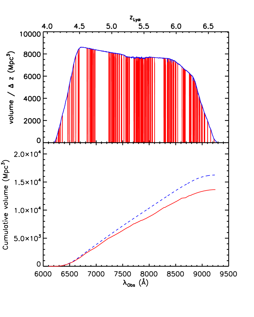
Figure 1.— The top panel shows differential volume (per unit redshift) as a function of wavelength for our 12 DEIMOS masks in the Cl1604 field. The vertical lines represent regions straddling bright night sky emission features. The lower panel shows the cumulative volume of the survey as a function of wavelength as corrected for the volume lost by the night sky emission lines (red solid line) and the uncorrected volume (blue dashed line).

2.3. Flux Calibration

The DEIMOS spectra were flux calibrated using a fifth-order Legendre polynomial fit to time-averaged DEIMOS 1200 l mm^-1 observations of spectrophotometric standard stars taken between June 2002 and September 2002 (see Figure 2). While the response is known to vary as a function of time, it is a relatively small effect under photometric conditions ($\sim$5%-10%). As most of our data were taken under photometric conditions, we can safely ignore this variation. The throughput correction for each pixel is:

$$f_{\lambda,i}[\frac{ergs}{cm^{2}\,s\,\AA}]=\frac{C_{i}\,D_{i}\,h\,c}{\pi 449^{2}\,\delta_{\lambda,i}\,t_{exp}\,\lambda_{c,i},}$$ (1)

where $C_{i}$ are the raw counts in the $i$th pixel, $D_{i}$ is the throughput correction at the central wavelength of the $i$th pixel, 449 is half the effective Keck II mirror aperture in centimeters, $\delta_{\lambda,i}$ is the plate scale in the $i$th pixel in Å pixel^-1, $t_{exp}$ is the effective exposure time, and $\lambda_{c}$ is the central wavelength of each pixel in Å.

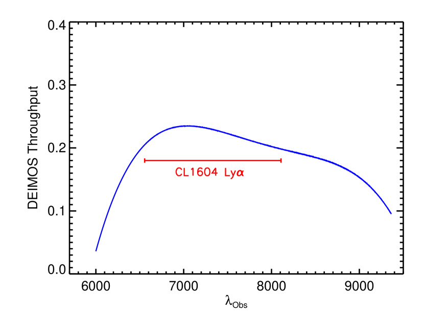
Figure 2.— A fifth-order Legendre polynomial fit to measured values of the throughput of DEIMOS for our spectral setup as a function of wavelength. This throughput includes loss from other optical elements and atmospheric transmission. For comparison the wavelength range of Cl1604 LAE candidates found in the data is plotted below the throughput curve. The wavelength range of LAE candidates encompasses the area of highest instrumental throughput.

The accuracy and precision of the throughput correction was checked in the following way. For each high quality target galaxy at the redshift of the supercluster, the spectrum was multiplied by a fit to the Sloan Digital Sky Survey (SDSS) $i\arcmin$ filter curve using a quadratic interpolation to match the wavelength grid of each DEIMOS spectrum. Targets were chosen because they were centered widthwise on the slit (serendipitous detections could fall anywhere on the slit) and supercluster members were chosen because the range of half-light radii was well determined from the ACS imaging.

A simulation was run in order to account for losses of light due to the finite spatial extent of the slit. Galaxies were simulated with exponential disk luminosity profile, half-light radii ranging from 0.34$\arcsec$ to 0.6$\arcsec$, based on values measured from ACS F814W data. For each simulated galaxy, the light profile was convolved with a Gaussian of FWHM comparable to the average seeing conditions under which our data were taken (0.9$\arcsec$). A slit of width 1$\arcsec$ and length 6$\arcsec$ was then placed on the galaxy, with the central part of the galaxy coincident with the central location of the slit. The total flux inside the slit was calculated for each simulated galaxy, with the slit throughput defined as the ratio of this quantity to the total flux in the absence of a slit. This slit throughput is plotted as a function of half light radius ($r_{h}$) and seeing in Figure 3. In addition, a similar simulation was run to determine the slit throughput as a function of position from the slit center under a variety of different seeing conditions. Since we are most interested in this effect for LAE galaxies, an object with $r_{h}=0.2\arcsec$ was used in the simulation, representing a reasonable limit to the sizes of large LAEs (see Overzier et al. 2006 or Venemans et al 2005).

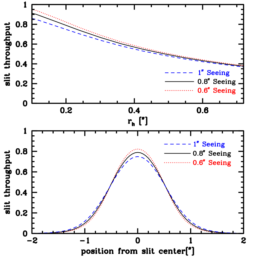
Figure 3.— Slit throughput ($\omega$) plotted as a function of half light radius (r_h) for a variety of different seeing conditions assuming the object is placed at the center of the 1$\arcsec$ slit (top panel), representing an absolute lower limit on the amount of flux that must be lost by any galaxy when observed with our spectral setup. The lower panel plots the loss of flux as a function of position along the minor axis (perpendicular to the spatial axis) of the slit for a galaxy with a half light radius of large LAEs (r_h=0.2$\arcsec$) for a variety of different seeing conditions. While the slit throughput has a moderately weak dependence on seeing and half light radius, the dependence on slit position is strong, falling off steeply when the object’s position is more than 0.4$\arcsec$ from the central position of the slit.

Despite the functional dependence of slit-loss on the object’s half light radius, the dependence is not particularly steep. For objects with $r_{h}$ $\leq$ 0.4$\arcsec$ the dependence is essentially linear. Thus, an average slit loss (1 - slit throughput) of 0.4 was adopted to correct each spectrum. Adopting an average slit loss correction was essential for the significant portion of DEIMOS objects which fall outside the coverage of the ACS mosaic and have no reliable half light radius measurements.

The flux density observed in the $i\arcmin$ bandpass for each spectrum is:

$$\overline{f_{\lambda}}=\frac{\sum_{i=0}^{n}f_{\lambda,i}S_{\lambda,i}\delta_{\lambda,i}\lambda_{c,i}}{c\sum_{i=0}^{n}\frac{S_{\lambda,i}\delta_{\lambda,i}}{\lambda_{c,i}},}$$ (2)

where the sum is over the $n$ DEIMOS pixels that fall within the $i\arcmin$ bandpass and $S_{\lambda,i}$ is the $i\arcmin$ transmission as a function of wavelength. The AB magnitude of each spectrum in the $i\arcmin$ band was then calculated by:

$$i\arcmin_{AB,spec}=-2.5log(\overline{f_{\lambda}})-48.60-\gamma\cdot sec(z),$$ (3)

with $\gamma$ being the airmass term for Mauna Kea. This spectral $i\arcmin_{spec}$ magnitude was then compared to our Palomar Large Format Camera (LFC; Simcoe et al. 2000) photometry (see G08 for details). Since the slit positions were determined from the LFC imaging, there were cases where there were noticeable ($>$ 1$\arcsec$) positional errors. Thus, galaxies not centered or absent from the slit or those with photometric flags were removed from the sample. The derived spectral magnitudes of the remaining galaxies are plotted against the LFC photometric magnitudes in Figure 4.

Figure 4.— LFC $i\arcmin$ magnitudes plotted as a function of magnitudes derived from the flux calibrated DEIMOS spectra (top panel) and as the difference between the spectral and LFC magnitudes (bottom panel) for all high quality (Q$\geq$3) spectra in the Cl1604 supercluster. The best-fit relations are overplotted. The systematic offset between the spectral and LFC magnitudes in the brighter end of the lower panel is most likely due to an underestimation of slit losses or non-photometric considerations. This is not problematic as the offset drops to zero at the fainter end of the plot, the region that our LAE candidates populate. The large rms in the lower panel represent real uncertainties in flux calibration of the data, a trend that does not improve with decreasing brightness.

The rms scatter of the spectral magnitudes between $i\arcmin$ = 19.5 and $i\arcmin$ = 25 is 0.49 magnitudes, corresponding to an $\sim$ 60% uncertainty in any absolute flux measurement. While the range of magnitudes are brighter than the average magnitude (or magnitude limit) of the LAE candidates in our sample, we adopt this rms as being reflective of the uncertainty in Ly$\alpha$ line flux measurements. In addition, the spectral magnitudes are systematically fainter on average by 0.48 magnitudes (lower panel of Figure 4). While this offset also corresponds to a bias of $\sim$ 60% for absolute flux measurements, this is less of a concern than the rms scatter for several reasons. First, the trend in the systematic offset as a function of magnitude tends towards zero at fainter magnitudes. If a magnitude-size relation is assumed for our target galaxies, the observed trend suggests that any offset comes from underestimating slit losses for the brighter target galaxies. Since we are interested in Ly$\alpha$ line fluxes, emission which originates from host galaxies that have typical $i\arcmin$ magnitudes fainter than our dimmest target galaxy (i.e., $i\arcmin$ $>$ 25.2), this systematic will not adversely affect our measurements. While we use a slit throughput of 0.8 (see the following section) when calculating the line fluxes for the purposes of deriving LAE properties such as EWs or SFRs, a full slit loss simulation used in calculating the luminosity function is undertaken in Section 5.4. Finally, we approach all measurements from the bottom—,i.e., erring on the side of underestimating the true flux of the galaxies so that our measurements will be a strict lower limit to compare with other surveys. We therefore ignore this systematic and include only the rms error when calculating line fluxes.

2.4. Line Flux Measurements

For each single emission line galaxy, the one-dimensional spectrum was inspected, and three bandpasses were chosen to measure the emission line flux. The first bandpass encompasses the entirety of the emission line, avoiding any instrumental or reduction artifacts. The other two bandpasses were chosen to be relatively sky line free regions blueward and redward of the emission line, as close to the emission line in the dispersion dimension as the data would allow, set to a minimal width of 20 Å. A linear model was fit to each spectrum in the blueward and redward bandpasses to mimic the continuum throughput. The model parameters were fit with a $\chi^{2}$ minimization routine, with the associated errors calculated from the covariance matrix. While a continuum fit was typically unnecessary for LAE objects, as the associated background was formally consistent with zero in most cases, the above procedure was implemented to accurately measure the line flux of low-$z$ single-emission line galaxies used as a comparison (see Section 3).

The resulting model background was subtracted from each spectrum in the emission line bandpass, with the total flux in each bandpass measured by:

$$F_{Ly\alpha}[\rm{\frac{ergs}{cm^{2}\,s}}]=\sum_{i=0}^{n}\left(f_{\lambda,i}\,\delta\lambda_{i}-B(\lambda_{i})\right)\,\frac{1}{\omega_{slit},}$$ (4)

where $B(\lambda_{i})$ is the model at each wavelength, $\delta\lambda_{i}$ is the size of the pixel at each wavelength, $\omega_{slit}$ is the slit throughput, and $f_{\lambda,i}$ is defined in Equation 1. The slit throughput used in the calculation of the Ly$\alpha$ line fluxes was set to 0.8, appropriate for a target galaxy with a half-light radius of 0.2$\arcsec$ in 0.9$\arcsec$ seeing. As most LAE candidates are not in the middle of the slit (as a target would be) and since the slit-throughput function remains below 80% for galaxies centered on the slit for all but the smallest half-light radii ($r_{h}\lesssim 0.1\arcsec$), the flux measured in this way still represents a lower limit to the true flux coming from the galaxy. Tables 1 and 2 list the name, redshift (assuming the line is Ly$\alpha$), right ascension and declination (assuming the serendip is at the center of the slit widthwise), the confidence class, line flux (minimally corrected for flux losses due to the slit as in the above equation), line luminosity, measured or 3$\sigma$ limiting magnitudes, the EW of the Ly$\alpha$ line, and the observed wavelength of each LAE candidate.

The associated errors for each flux measurement were derived from a combination of (response corrected) Poisson errors from each spectrum and the errors associated with the background model, as well as the flux calibration error discussed in the previous section. There can also be significant systematic errors associated with the bandpass choices. Limiting the size of the emission line bandpass can significantly underestimate the true line flux, while an overextension of the limits can introduce significant noise into the measurement. A select group of galaxies, spanning the dynamic range of the spectra measured in this manner, were analyzed in order to estimate the magnitude of this error. In all cases the systematic errors derived for a “reasonable” range of bandpass choices were completely dwarfed by Poisson errors.

2.5. Flux Limit and Spectral Completeness

Since our search depended almost entirely on human detection of sources, accurately quantifying the completeness limit of the objects detected is more difficult than in searches that use automatic peak finding algorithms. The human eye, while being very good at discriminating between spurious and real detections and at finding irregularities in data (serendips in our case), is subject to a variety of effects which are difficult to quantify. To roughly quantify our completeness limit we simulated one hundred slits, each 55 by 8192 pixels corresponding to 6.5$\arcsec$ by 2700 Å at the DEIMOS 1200 l mm^-1 grating plate scale. These data were first simulated using the noise and background properties measured from actual DEIMOS two-dimensional spectra in regions where features and poor-sky subtraction were absent. These feature-free, artifact-free regions were collapsed into one-dimensional spectra using the same method used by spec2d in extracting one-dimensional spectra of target galaxies. Each of the two-dimensional spectra were populated with flux values that mimicked the properties of the real two-dimensional spectra, creating in essence one-hundred 6.5$\arcsec$ “blank-sky” slits. These simulated blank-sky slits were populated with objects that varied in both intensity and frequency. For each simulated slit, between zero and four objects were placed on the slit, characterized by two-dimensional Gaussians with freely varying amplitudes, dispersions in both the spatial and spectral dimensions, spatial locations, and central wavelengths. Noise was also introduced to each Gaussian to properly simulate the counting error associated with observing actual galaxies. The slits were populated so that a slit had zero objects 50% of the time and between one and four objects 50% of the time. In addition, the heights and dispersions of the Gaussians were constrained so that the objects would have reasonable flux values, i.e. values corresponding to an order of magnitude both fainter and brighter than the faintest and brightest single-emission line object detected in our data.

Each of the two-dimensional slits was then analyzed by one of the authors (BL) in blind observations using a fashion similar to that used for the original data. The conditions that were present when observing the original slits were re-created to the best of our ability (e.g., the time spent on each slit, the method of looking for detections, the software used). For every simulated object detected in the two-dimensional slits, a one-dimensional spectrum was created using methods similar to spec2d. A catalog of generated objects was compared to the catalog of objects detected by eye and the remaining objects that went undetected in the data were then similarly extracted. If we set the completeness limit at the faintest object detected nearly 100% of the time, this limit corresponds to objects with significances between 105$\sigma$ and 111$\sigma$ in the two-dimensional data, or a one-dimensional significance of 7$\sigma$. This significance translates to a completeness limit of $1.9\times 10^{-18}$ ergs s^-1 cm^-2 for a 7200s exposure time, decreasing slightly for our masks with longer integration times. This completeness limit is consistent with the line flux analysis done in Section 3.3 (see Figure 8 and associated discussion), suggesting that this limit is close to the actual completeness limit of the survey.

3. Emission Line Tests

The large spectral coverage and moderately high resolution of DEIMOS give us a distinct advantage over narrowband imaging searches for LAEs or searches with small spectral coverage, as we are able to differentiate the Ly$\alpha$ line from other emission lines that are typically confused for it. The lines which are the most prevalent contaminants in searches for Ly$\alpha$ emission are the 3727 Å  [OII] doublet, [OIII] at 5007 Å, H$\beta$ at 4861 Å, or H$\alpha$ at 6563 Å.

The most insidious contaminant in many LAE surveys is the [OII] doublet (rest frame separation 2.8Å). For our spectral setup this line would be observed at a redshift of 0.71 $\leq$ $z$ $\leq$ 1.41 and is usually resolved with the 1200 l mm^-1 grating. A small fraction of the [OII] doublets are unresolved due to a combination of galactic rotational effects and the slit being oriented along the major axis of the galaxy. In this case the [OII] line can still be discriminated from Ly$\alpha$ by the asymmetry of the line. The nebular Ly$\alpha$ line is typically characterized by its strong asymmetry, with suppression of line flux in the blueward portion and, in some cases, an extended redward tail. A blended (unresolved) [OII] line in normal star forming regions (in the absence of an active galactic nucleus (AGN)) exhibits asymmetry opposite that of Ly$\alpha$, with an extended tail in the blueward portion of the line (Osterbrock 1989; Dawson et al. 2007). Galaxies emitting H$\alpha$, H$\beta$, or [OIII], in cases of even moderate S/N, can be easily distinguished from Ly$\alpha$ by other associated spectral features. The 5007 Å [OIII] line is typically seen with 4959 Å [OIII] and 4861 Å H$\beta$ with varying degrees of relative intensities (Baldwin et al. 1981). The 6563 Å H$\alpha$ line can be identified by two accompanying SII lines at 6716 Å and 6730 Å and two [NII] lines at 6548 Å and 6583 Å, also with varying degrees of relative intensity. Many spectra originally classified as single-emission line objects were recognized as low redshift interlopers through the identification of faint associated lines.

For the remaining 39 objects that were classified as genuine single-emission line objects, several tests were performed to further remove any low redshift interlopers. The Ly$\alpha$ line is characterized by a large 1.3–4.5 mag continuum break blueward of the line due to attenuation of Ly$\alpha$ photons by intervening neutral hydrogen (H04). Initially, the spectral data were inspected, and 10 single-emission line serendip exhibiting appreciable continuum blueward of the emission feature relative to any redward continuum was eliminated as a potential LAE candidates. The imaging data were also useful in discriminating single-emission line serendips in this regard, as the photometric filter setup would also, in many cases, probe the continuum break across the Ly$\alpha$ line (see Figure 5). Each single-emission line serendip detected in one or more of the photometric bands was required to exhibit a continuum break over filters blueward and redward of the line. Since most of these objects are extremely faint in the imaging (if they are detected at all), requiring a strong continuum break over the emission line is, in almost all cases, similar to requiring that the object drop out of any band blueward of the emission line. Our bluest LFC and ACS bands, $r\arcmin$ and F606W, are situated so that either would pick up a significant amount of continuum flux from any LAE at the bluer end of our detection limit ($\lambda$ $\leq$ 7000 Å, $z_{Ly\alpha}$ $\leq$ 4.75). For objects such as this we had to rely on Subaru Suprime-cam V-band data to discriminate between potential LAEs and low-$z$ interlopers. Any galaxy detected in the V-band data was excluded as an LAE candidate due to the relative shallowness of the image (see Section 4.1 for details on the depth of the photometry). All but two of 22 single-emission line galaxies that were eliminated as potential LAE candidates through the above tests failed the continuum break test. The two single-emission line low-$z$ interlopers that did not fail this test were among the 10 galaxies that failed the spectral continuum break test. In addition, each single-emission line serendip that was detected in the photometric data was also inspected visually, and any objects with large ($>$ 2$\arcsec$) angular extents were classified as low-$z$ interlopers. Six of the 22 single-emission line low-$z$ interlopers were rejected by this test, although in all cases these galaxies had failed at least one of the two previous tests.

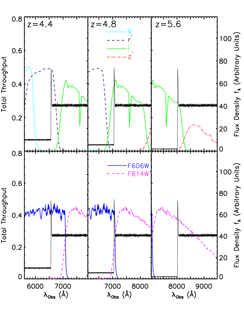
Figure 5.— Synthetic Ly$\alpha$ spectra at three different redshifts spanning the range of redshifts of our sample overlaid on the four ground-based filter transmission curves (top three panels) and two ACS filter transmission curves (bottom three panels) for which we have coverage. The continuum break over the Ly$\alpha$ line is modeled based on narrowband imaging measurements of the continuum break (H04). For lower redshift LAEs, the only band able to detect the continuum break is the ground-based V band. At the redshift of most of our sample ($z\sim 4.8$), the Ly$\alpha$ line just passes the coverage of the ground-based $r\arcmin$ band and lies just at the red end of the F606W band. At higher redshifts the Ly$\alpha$ line is comfortably situated in the F814W band and at the red end of the ground-based $i\arcmin$ band, giving us significantly more power to discriminate between interlopers and genuine LAEs at these redshifts. The throughput of the V band is scaled down and the throughput of the $z\arcmin$ band is scaled up for clarity.

Of the original 39 single-emission line cases, 17 objects survived the previous tests. A small subset of these objects were insensitive to these tests, as the single-emission line object was superimposed spatially in the spectral data with either the target or another serendip. In such cases, the single-emission lines were checked against a variety of nebular emission lines at the redshift of the superimposed target or serendip to verify that it could not simply be an unusual emission feature coming from the same galaxy. In many cases, however, it was clear from the morphology or positions of the lines that the two emission features originated from two separate sources. In some cases the two superimposed objects were resolved in the ACS data, and the continuum break test was used on one or both of the galaxies, depending on whether the identity of the single-emission line source was certain. More frequently, however, the two objects remained unresolved in the HST data, so we include them in our sample. Of the 17 objects that survived the original single-emission line tests, all 17 passed the tests described above. These 17 objects comprise our LAE sample (see Figures 19-21).

3.1. Line asymmetry

Another discriminator used on the individual single-emission line spectra was a computation of the wavelength asymmetry parameter (Dawson et al. 2007). Briefly, the asymmetry parameter, a_λ, is defined as:

$$\frac{1}{a_{\lambda}}=\frac{\lambda_{c}-\lambda_{10,b}}{\lambda_{10,r}-\lambda_{c},}$$ (5)

where $\lambda_{c}$ is the central wavelength of the emission, defined as the point of maximal flux in the line profile, and $\lambda_{10,r}$ and $\lambda_{10,b}$ are the wavelengths where the flux first exceeds 10% of the peak flux redward and blueward of the line, respectively. This diagnostic can be used to further discriminate single-emission lines that exhibit standard Gaussian (Voigt) profiles such as H$\beta$, H$\alpha$, [OIII] (1/$a_{\lambda}$ $\sim$ 1), or a blended 3727 Å  [OII] doublet (1/$a_{\lambda}$ $>$ 1) from a higher redshift Ly$\alpha$ line that exhibits strong asymmetry in the opposite direction. While this test can be a useful diagnostic in a statistical sense, an asymmetry parameter of $1/a_{\lambda}$ $\geq$ 1 was not a strong enough constraint to rule out an object as an LAE candidate if it had passed all the previous tests. This is because several processes (instrumental broadening, local underdensities of HI regions, etc.) can cause the LAE emission to appear symmetric. Conversely, an object which had failed one or more of the above tests was not reclassified as a potential LAE based on an unusually high (1/$a_{\lambda}$ $<$ 1) asymmetry parameter, as low redshift lines can, under rare circumstances, exhibit strong redward-skewed asymmetry (see for example object D21 in MS04). Therefore, this diagnostic was used only to discriminate between high quality LAE candidates and poorer quality candidates, rather than distinguishing genuine LAEs from interlopers. Figure 6 shows a histogram of the inverse of the asymmetry parameter of the known lower redshift single-emission line objects, a population of blended [OII] emitters (confirmed by other associated lines present in the spectrum), and our 17 LAE candidates. The objects clearly separate out; the LAE candidates primarily occupy the high asymmetry (low inverse asymmetry) portion of phase space, the low-$z$ interlopers are distributed around unity (symmetric), and the [OII] galaxies are primarily situated in the region of phase space opposite that of the LAE candidates. In fact, all but three LAE candidates (all Quality 1; see below) have inverse asymmetry parameters less than 0.75.

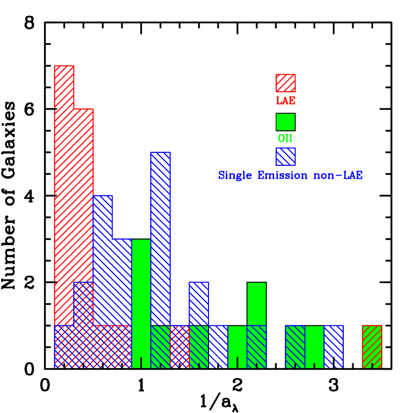
Figure 6.— The inverse of the asymmetry parameter measured for the emission lines of three different populations: known blended [OII] emitters ($0.7<z<1.4$), low-$z$ single-emission line galaxies, and our 17 LAE candidates. This parameter easily discriminates even blended [OII] emission lines, which are strongly skewed toward high values of the inverse of the asymmetry parameter, from LAE lines which typically exhibit values much less than unity. The low-$z$ single-emission line galaxies are less easily discriminated by this test, with a distribution that is centered around symmetric (1/a_λ=1) line profiles and wings that extend into the phase space of the other two populations. All LAE candidates with higher inverse asymmetries (1/$a_{\lambda}>0.75$), including one very high value, are low-quality candidates.

3.2. LAE Confidence Classes

Each of the 17 LAE candidates was assigned a quality class. Quality classes are assigned to LAE candidates in a fashion nearly identical to that of S08 and are defined as follows: Quality 1 objects pass all of the above tests, but show no additional indicators of being genuine LAEs. Objects which are Quality 1 do not exhibit any asymmetry (or exhibiting blueward-skewed asymmetry) in their line profiles and are non-detections in all photometric bands. These objects are our least secure candidates, nearly equally likely to be low luminosity foreground galaxies as LAEs. Quality 2 and 3 objects all similarly pass the interloper tests but also show strong asymmetric line profiles. A few of these objects are detected in one or more photometric bands, further increasing our confidence in these objects as genuine LAEs, but it is the asymmetric line profile which is the defining characteristic of the higher confidence classes. Both Quality 2 and Quality 3 candidates represent our highest level of confidence that an object is a genuine LAE. However, Quality 2 objects are superimposed with a target or another serendip spatially on the slit. Thus, the flux measurements of the Quality 2 objects could be significantly dimmed by extinction from the interstellar medium (ISM) of the foreground galaxy or boosted through galaxy-galaxy lensing. This additional, unknown component of the uncertainty makes it necessary to exclude Quality 2 galaxies from certain parts of the analysis.

3.3. Flux and Redshift Tests

The tests discussed in the beginning of Section 3 can only be used to rule out objects as LAEs, not to prove that any particular object is definitively an LAE. The tests in the following two sections explore the statistical similarities or differences between LAE candidates and the low-$z$ interlopers, giving us further confidence that the LAE candidates represent a unique and separate population.

3.3.1 Effective Redshift Test

First we compare the observed wavelengths of the single-emission lines in the low-$z$ interloper population to the observed wavelengths of the Ly$\alpha$ lines in the LAE candidates. The low-$z$ single-emission line interlopers are comprised of some combination of [OII], H$\beta$, [OIII], and H$\alpha$ emitters and therefore cannot be given definite redshifts. Following the analysis done in S08, we have recast the low-$z$ interlopers in terms of an effective redshift: the redshift that the object would have if the line were Ly$\alpha$, such that $z_{eff,Ly\alpha}$ = ($\lambda_{em}$/1215.7 - 1).

The idea of this test is that the low-$z$ single-emission line interlopers, if they truly are comprised of a mix of the aforementioned lines, should be, in the absence of any instrumental effects, equally distributed in effective redshift (wavelength) space. An object at a redshift of $z$ = 0.35 emits the 5007 Å[OIII] line at $\lambda_{obs}$ = 6759 Å and 6563 Å  H$\alpha$ at $\lambda_{obs}$ = 8860 Å, both of which could mimic single emission lines under a variety of different conditions. These effects could be (1) instrumental: the placement of the slit on the slit mask truncating either the blue or red end of the CCD response; (2) atmospheric: a bright night sky line masking the second emission line; or (3) a result of galactic processes: a low level AGN which exhibits strong [OIII] emission but little to no Balmer emission, or a starburst galaxy having strongly suppressed forbidden transitions relative to the strength of the Balmer lines. In any of these cases, the chance is more or less equal that the single-emission line galaxy will show up as the blue or the red emission line. The redshift distribution of the LAE population should be strongly biased towards the lowest redshifts to which we are sensitive, as we probe successively shallower in the luminosity function as the LAEs move to higher redshifts. Thus, if the LAE population represents a truly different population than the low-$z$ single-emission line interlopers, the redshift histograms should differ significantly.

Figure 7 shows the comparison in effective redshift space between the 22 low-$z$ interlopers, the 4 Q=1 and the 13 Q=2,3 LAE candidates. The low-$z$ single-emission line interlopers are more or less evenly distributed across $z_{eff,Ly\alpha}$ with two important exceptions. There are no interlopers shortward of $z_{eff,Ly\alpha}$ = 4.4, possibly due to the prevalence of H$\alpha$ as the unknown single emission line in the interloper population. The rest wavelength of the H$\alpha$ line has $z_{eff,Ly\alpha}$ = 4.398 so if the interloper population does consist primarily of $H\alpha$ emitters, few galaxies would be seen blueward of this limit. Another reason for this drop-off in detections could be the significant drop in DEIMOS sensitivity blueward of $\sim$ 6600 Å  for our spectral setup. The second drop-off in detections occurs at $z_{eff,Ly\alpha}$ $>$ 6.1, most likely due to the significant decrease in DEIMOS sensitivity and the decrease in significant sky line free spectral windows redward of $\sim$ 8700 Å (see Figure 2).

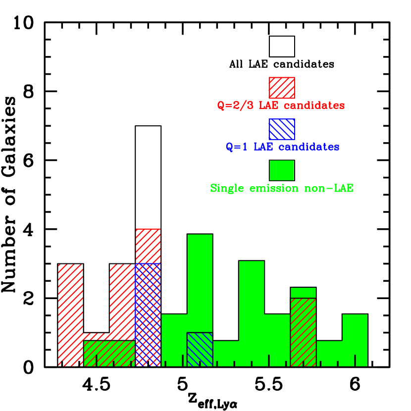
Figure 7.— Redshift histogram of the high quality (Q=2,3) and low quality (Q=1) LAE candidates. A strong peak can be seen at $z\sim 4.8$ as well as less pronounced peaks at $z\sim 4.4$ and $z\sim 5.7$. Conversely, the overplotted low-$z$ interloper population (plotted in terms of $z_{eff,Ly\alpha}$; see Section 3.3.1) is distributed nearly symmetrically around $z\sim 5.1$, with a much slower falloff at high redshifts.

The LAE population is strongly peaked towards the low end of our redshift sensitivity. A very noticeable peak exists at $z\sim 4.8$, which may represent a real clustering of the LAE population in projection space or could simply be an artifact of the sensitivity issues discussed in the previous paragraph, as the DEIMOS sensitivity peaks at $\sim$ 7000 Å  for our setup. More likely, it is some combination of these two effects (see Section 5.2 for a discussion). The Q=1 LAE candidates, which are our least secure candidates, are surprisingly consistent with our higher confidence Q=2,3 population, also peaking around $z_{Ly\alpha}$ $\sim$ 4.8. There are two Q=2,3 candidates at $z\sim 5.7$ which are unexpected, given our prediction that the LAE population should be strongly peaked towards the low-redshift end.

3.3.2 Line Flux Test

The second of these tests explores the possibility that the LAE candidate population represents a lower luminosity subset of the single-emission line interlopers. A majority of single-emission line interlopers were ruled out by broadband detections, i.e., not exhibiting a sufficiently strong continuum break over the feature to be plausibly identified as Ly$\alpha$. All of the single-emission line interlopers were detected in the photometry. Conversely, the majority of the LAE candidate population were not detected in any of the three LFC bands nor the two ACS bands. Thus, the LAE candidate population clearly represents a class of objects that are significantly dimmer in continuum luminosity. If the LAEs are truly drawn from the same population as the low-$z$ interlopers, their line luminosities should similarly scale down. This test provides a quantitative statistical tool to differentiate the LAE candidates from the lower luminosity tail of the single-emission line interloper luminosity function. This test is not sensitive to the case where the LAE candidates represent a population of dwarf starbursting galaxies with higher line luminosity relative to their continuum brightness (Fricke et al. 2001; Guseva et al. 2003; Kehrig et al. 2004; Izotov et al. 2006).

Figure 8 shows the comparison between the line fluxes of the single-emission line interlopers relative to the LAE candidates. The Q=2,3 LAE candidates are, on average, brighter than the single-emission line interloper objects, with the mean line flux about 0.5 dex higher than the interloper population. The average magnitude of the interloper population in the band which best samples the continuum emission near the emission feature is 23.5 mags. In contrast we can adopt the LFC $i\arcmin$ 3$\sigma$ limit of 24.3 mags as the upper bound on the continuum flux of LAEs that are not detected in the photometry (a conservative limit as many of the candidates are undetected in the ACS images which have a 3$\sigma$ depth of $\sim 26$ mags). This limit on the continuum flux requires the LAE candidates, if they are instead low-luminosity, low-$z$ interlopers, to have line equivalent widths (EWs) at least 10 times greater than the average EW of the known single-emission line interlopers (5.4 Å). Such high EWs are certainly plausible in dwarf galaxies undergoing a starbursting event where the EWs of H$\alpha$ (usually the strongest lines in optical starbursting spectra) are the range 50-150 Å (Kennicutt 1998, Petrosian et al. 2002) and have been measured as high as $\sim$1500Å (Kniazev et al. 2004, Reverte et al. 2007). However, such objects are uncommon, and we would expect to observe other associated lines (e.g., [NII], H$\beta$, [OIII]) in the data, which we do not. It is interesting to note that if we adopt a standard ratio for log$[L([NII]$ 6585 Å$)/L(H\alpha)]$ and log$[L([OIII]$ 5007 Å$)/L(H\beta)]$ of -0.45 for star-forming galaxies (Baldwin et al. 1981; Brinchmann et al. 2004; Shapley et al. 2005; Yan et al. 2006), the bulk of our LAE candidates ($\sim$60%) are sufficiently brighter than the completeness limit so that the associated lines would be detected if the emission were instead H$\alpha$ or H$\beta$.

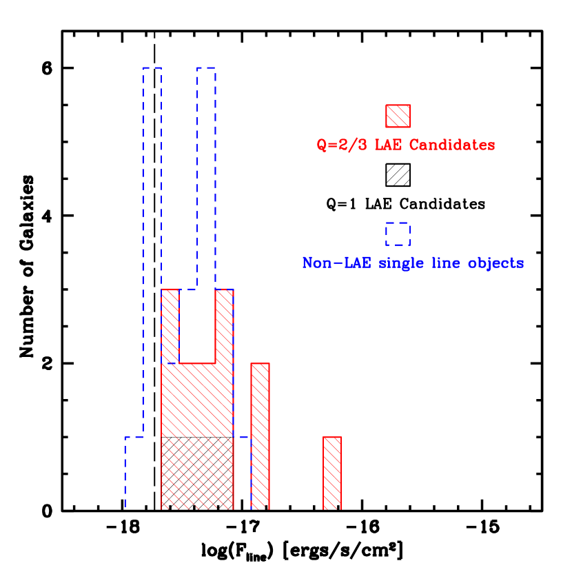
Figure 8.— Histogram of line fluxes uncorrected for slit losses of our LAE candidates and confirmed low-$z$ single-emission line objects. While the two distributions overlap, the low-$z$ interloper population is characteristically dimmer than both the high (Q=2,3) and low (Q=1) quality LAE candidates. The difference in the observed distribution suggests that the LAE candidates are not primarily comprised of low luminosity single-emission line objects at low ($z<1.4$) redshifts. The vertical long dashed line represents our adopted completeness limit of $1.9\times 10^{-18}$ ergs s^-1 cm^-2

The Q=1 LAE candidates are essentially identical to the fluxes of the low-$z$ interloper population, with a mean flux of $4.8\times 10^{-18}$ ergs s^-1 cm^-2 as compared to the mean flux of the interloper population of $3.9\times 10^{18}$ ergs s^-1 cm^-2. While this similarity may be an indication that the Q=1 LAE candidates contain at least some low-$z$ interlopers mixed in with genuine LAEs, it also may be misleading. The average upper limit on the magnitude of the Q=1 candidates in the filter sampling the continuum surrounding the emission feature is 24.9, nearly 1.5 magnitudes dimmer than for the single-emission line counterparts. While the line fluxes of these two populations are similar, the EW of the $Q$=1 LAE candidates would still necessarily have to be a factor of 4 higher than the interloper population. In addition, the Q=1 line fluxes fall near the completeness limit of $1.9\times 10^{-18}$ ergs s^-1 cm^-2 and near the low-flux tail of the line flux measurements of the high quality (Q=2,3) LAE candidates. We would expect, independent of the redshift range, an inverse relationship between the number of detections and the line flux down to the completeness limit and a steep falloff in detections thereafter. If the Q=1 LAE candidates constitute real detections of genuine LAEs, this would be the behavior we observe in the data. Thus, it may be that these low quality candidates simply represent the fainter flux end of the LAE population, and their lower S/N prevents them from reliably being classified as high quality candidates.

3.4. Composite Spectra

Previous tests focused on measurements of individual spectra of galaxy signatures at or near the flux limit, making these measurements susceptible to noise effects. While we compare the ensemble properties of the galaxy populations, which is less sensitive to noise variations in the data than the comparison of individual measurements, an alternative is co-adding of the spectra in order to increase the S/N.

Figure 9.— Composite spectrum of the LAE candidates and the known low-z interlopers smoothed with a Gaussian smoothing kernel of $\sigma$=1.5 pixels. Each co-addition is done using luminosity weighting (see the text). The dashed lines show Gaussian fits to the line profiles. Both the high (Q=2,3) and low (Q=1) quality LAE candidates are poorly fit by a Gaussian model.

To properly retain the overall spectral properties of the constituent objects (e.g., line shapes, resolution, velocity dispersions, etc.) and to avoid averaging out faint features, it is necessary when coadding galaxies to determine the redshift as accurately or in as consistent a manner as possible. While we were able to determine redshifts for our interloper sample through the centroiding provided by spec2d, the LAE population was problematic because of the uncertainty in determining the true peak of the line. In the absence of any other knowledge about the true profile of the Ly$\alpha$ emission in each galaxy (other than its asymmetry), the assumption was made that the wavelength associated with the peak flux in each emission line profile represented the central wavelength for that emission. Lack of knowledge about the shape of the true line profile introduces a significant ($\delta_{z}\sim 0.002$) absolute error in the redshift measurements. However, since this measurement is made in a consistent way for each spectrum, the relative error in the redshifts (the important quantity for coadding purposes) between any two spectra is quite small. Thus, any asymmetry in the original line profiles should be preserved through this process.

Each galaxy spectrum was then “de-redshifted” to its rest frame, or, in the case of the single-emission line interlopers, the effective rest frame (see Section 3.3). Each rest frame spectrum was interpolated onto a pixel grid of common size, chosen to subsample the lowest (rest-frame) pixel scale. The resulting spectra were then added together in the following two ways: (1) each spectrum was normalized by the galaxy’s total spectral flux (uniform weighting), or (2) galaxies were added together with no normalization (luminosity weighting). In both cases, the flux of each pixel in the co-added spectrum was populated using a Poissonian variance weighted mean of the pixel values at each wavelength in the individual spectra.

Figure 9 shows the luminosity-weighted coadded spectrum for three different populations: the high quality (Q=2,3) LAE candidates, the low quality (Q=1) LAE candidates, and the known low-$z$ interlopers. The coadded spectrum of each set of galaxies was fit with a Gaussian, with the goodness of fit parameterized by the reduced $\chi^{2}$. As expected, the Gaussian model does a poor job at reproducing the observed line profile for the high quality LAE candidates ($\chi^{2}/\nu=2.38$). Conversely, both the low quality LAE candidates ($\chi^{2}/\nu=0.67$) and the low-$z$ interloper ($\chi^{2}/\nu=0.88$) population are statistically well fit by the Gaussian profile. Despite the statistical significance of the fit, visual inspection of the low-$z$ interloper population shows the line profile to be clearly more symmetric than the low quality LAE candidates, as should be the case if at least some of the low quality LAE candidates are real. Additionally, the best-fit Gaussian to the low quality candidates has a FWHM of 0.68 Å, nearly twice as large as the best-fit FWHM of the known low-$z$ interlopers, further suggestive that the lower quality LAE population contains at least some genuine LAEs. The inverse of the asymmetry parameter (Section 3.1) was also calculated for the luminosity-weighted co-added spectra of each of the galaxy subsets, with values of 0.35, 0.57, and 1.14 for the high-quality LAE candidates, low quality LAE candidates, and low-$z$ interloper population, respectively. Both of these results reinforce the conclusions reached from analyzing the individual spectra: that the high quality LAE candidates probably represent a real population of LAEs while the lower quality candidates probably represent some combination of genuine high redshift LAE galaxies and low-$z$ interlopers. The results of these calculations did not change significantly if we instead use uniform weighting.

4. Properties of the Cl1604 Ly$\alpha$ Emitters

4.1. Photometric Limits

The broadband photometry associated with the Cl1604 data set was designed almost exclusively to select spectroscopic targets for the supercluster at $\langle z\rangle=0.9$, sampling down to 3$\sigma$ limits of 24.8, 24.3, and 23.6 in $r\arcmin$, $i\arcmin$, and $z\arcmin$ respectively. These magnitudes were calculated by measuring the magnitude of a circular object with a 1$\arcsec$ diameter, where each pixel has signal equal to three times the sky rms (effectively a circular top hat profile). An aperture of 1$\arcsec$ was chosen to match the average seeing conditions from on Palomar mountain during our observations.

The depth of these observations are only sufficient to probe the continuum luminosities of the most massive galaxies at high redshift ($z\geq 4.4$). Indeed, only one of our LAE candidates (16XR1.72, an object that was subsequently picked as a spectroscopic target) was detected to the depth of these images. The accompanying archival Suprime-cam observations have a 3$\sigma$ limiting magnitude V$\sim$24.0 for the same choice of aperture as the other ground-based images. The exact value of this limit is unknown due to imperfect photometric calibration, though it is probably accurate to $\sim$0.2 mags based on comparisons between the measured Subaru magnitudes and overlapping fields with precise photometric calibration.

The ACS observations are significantly deeper, reaching 3$\sigma$ limits of 26.1 and 25.5 in F606W and F814W in most of the pointings and 26.8 and 26.3 in two deeper pointings centered on clusters A and B. Photometric limits in the ACS pointings are calculated for a 0.3$\arcsec$ circular aperture using the same method as the ground based limiting magnitudes. A smaller aperture was chosen because of the significant increase in resolution ACS provides relative to the ground based images. These 3$\sigma$ limits are conservative limits on the depth of our images as the differential number counts do not turnover (hereafter “turnover magnitude”) until magnitudes that are 0.1-0.2 fainter than the 3$\sigma$ limits of the ground-based data and 0.5-1 mags fainter than the limits of the ACS data. Even though the ACS data does not overlap the entirety of our spectral coverage, only two of our 17 LAE candidates (SC2NM1.45 and SC2NM2.61) fell outside the ACS area. Despite this, only three of the 15 LAE candidates that were covered by ACS pointings were detected in the ACS imaging.

In order to place limits on the broadband photometry in the absence of detections, local versions of $3\sigma$ limiting magnitudes were measured for each LAE candidate from the data using a method similar to the measurement of the 3$\sigma$ limiting magnitudes for each image. However, rather than measuring the rms over a large portion of the image, the rms was instead measured in a statistically significant region either at the central location of the galaxy (inferred from the spectroscopy, assuming the object was at the center of the slit) or near the target location if the object was superimposed spatially with the target. For $3\sigma$ limiting magnitudes in the ACS images, this rms value per pixel (corrected for correlated noise from pixel subsampling) was multiplied by the number of pixels covered by an object with a circular aperture of radius 0.21$\arcsec$. This number was motivated by the half light radius of LBGs (Steidel et al. 1996b; Ferguson et al. 2004) and intentionally designed to overestimate the limiting magnitude of such objects; all of the LAE candidates detected in the ACS imaging had detected magnitudes significantly dimmer than the corresponding $3\sigma$ limiting magnitude. In addition, the $3\sigma$ limiting magnitudes were measured with the Palomar LFC imaging using similar techniques. As before, a circular aperture of $1\arcsec$ was used in the LFC calculation, as a typical LAE would not be appreciably different spatial extent than a point source in the LFC images. Table 1 gives the $3\sigma$ limiting magnitudes of all the non-detected LAE candidates as derived from both the ACS imaging (when available) and the Palomar LFC imaging.

4.2. Equivalent Widths

The EW is typically calculated for the Ly$\alpha$ line in the following way (Dawson et al. 2004):

$$EW(Ly\alpha)=\frac{F_{Ly\alpha}}{f_{\lambda}(1+z),}$$ (6)

where $F_{Ly\alpha}$ is the total line flux in the Ly$\alpha$ line and $f_{\lambda}$ is the flux density redward of the Ly$\alpha$ emission, a formalization that is convenient for measurements of LAEs in narrowband imaging surveys.

Without proper detections of the continuum luminosity of a majority of our LAE candidates, calculating the EW of the Ly$\alpha$ line, something that is strongly dependent on the continuum luminosity, is not possible. Instead we calculate a lower bound on this quantity. Formally, our $3\sigma$ limiting magnitude represents a strict upper (brighter) bound on the continuum flux density. The uncertainty in the flux loss in the Ly$\alpha$ line due to the slit works in the same direction; the total line flux, minimally corrected for slit losses (see Section 2.4), represents a strict lower (dimmer) bound on the line flux. Thus, any calculation based on these numbers will represent a very conservative lower bound to the EW of the Ly$\alpha$ line in these galaxies.

In order for the EW measurement, or a lower bound to this measurement, to characterize the intrinsic properties of high-redshift LAEs, it is necessary to make some correction for attenuation from the intergalactic medium (IGM). This attenuation occurs primarily due to resonant scattering of redshifted Ly$\alpha$ photons in intervening clouds of neutral hydrogen. As such, only Ly$\alpha$ photons emitted by galactic components blueshifted with respect to the bulk velocity of the galaxy will be affected by this dampening. Although there can be, in principle, some contribution to the attenuation from intervening Helium and metal systems, such contributions are typically small in comparison (Madau 1995). The attenuation to the blueward flux solely from intervening HI regions was characterized most recently by Meiksin (2006), where the fraction of attenuated Ly$\alpha$ photons blueward of 1215.7 Å was given as:

$$f_{att,Ly\alpha,b}=1-exp\left(-5.8\times 10^{-4}\,(1+z)^{4.5}\right)\,\,(z>4),$$ (7)

where the argument of the exponential is the mean Gunn-Peterson optical depth for an object at a given redshift. Assuming the LAE is rotationally supported such that there is no skew in the velocity components of the Ly$\alpha$ emitting HI regions, the true flux of the Ly$\alpha$ line in LAEs (for z $>$ 4) is given by:

$$F_{corr,Ly\alpha}=\frac{F_{Ly\alpha}}{0.5+0.5(1-f_{att,Ly\alpha,b}),}$$ (8)

an expression that ignores any dust extinction of the Lyman continuum. While Equation 7 is derived from an average of different lines of sight from observed data, we use it here to correct on a galaxy by galaxy basis. Though making this correction may introduce significant bias to the EW measurement of a single galaxy, correcting our entire sample produces a distribution which more accurately reflects the true contribution of star-forming processes in these galaxies. After correcting each galaxy’s line flux using Equation 8, the upper bound of the continuum flux density, $f_{\lambda}$, was estimated. For the bulk of our sample which went undetected in the photometry, the flux density was estimated with both the $3\sigma$ limiting magnitude in the band encompassing the Ly$\alpha$ emission and in a band just redward of the Ly$\alpha$ emission. For the higher redshift galaxies ($z>5.5$), we had no bands completely redward of the Ly$\alpha$ line with sufficient depth to make a meaningful estimate of the EW with the LFC data (see Figure 5), as our $z\arcmin$ imaging was shallower than our other bands. Both cases the LAEs fall within the ACS imaging and we therefore use only the 3$\sigma$ magnitude limit in the F814W filter to estimate the flux density redward of the Ly$\alpha$ line.

Since these galaxies are undetected in the ACS or LFC data, both the EW measurement from a band encompassing the Ly$\alpha$ line and from a band longward of the Ly$\alpha$ line represent a reasonable approximation to the lower limit on the true EW. Although we formally calculate EWs from the 3$\sigma$ limits in bands containing the line, the true lower bounds to the EWs are characterized solely by the EWs calculated from the 3$\sigma$ limiting magnitudes of bands redward of the Ly$\alpha$ line. In addition, we have calculated the EWs using the turnover magnitude (see Section 4.1 for definition) in the ACS imaging. For the shallower ACS pointings this magnitude corresponds to 26.99 and 26.68 in F606W and F814W respectively, increasing to fainter magnitudes (27.76 and 28.01 in F606W and F814W) for the deeper ACS pointings. These turnover magnitudes are not to be confused with the completeness limits of the images, which must be constrained through simulations; however, the turnover magnitudes are likely a good approximation to the limit at which we are complete for LAE-size objects. While the EWs calculated using the turnover magnitudes are not strictly lower limits, they serve as more reasonable (less conservative) estimates of the lower bound of the Ly$\alpha$ EW (see Table 1).

For galaxies detected in the imaging (either ACS or LFC), the calculation was much more direct. While any measurement of the EW still represents a lower limit (due to the unknown amount of flux loss of the Ly$\alpha$ line from the slit), the redward continuum flux densities could be calculated in a straightforward way from the observed magnitudes. These measurements were done, as was the case for the undetected objects, for both the band encompassing the Ly$\alpha$ emission and a band redward of the line emission. The lower limits on these EWs are shown in Table 2, quoted at the 95% confidence level.

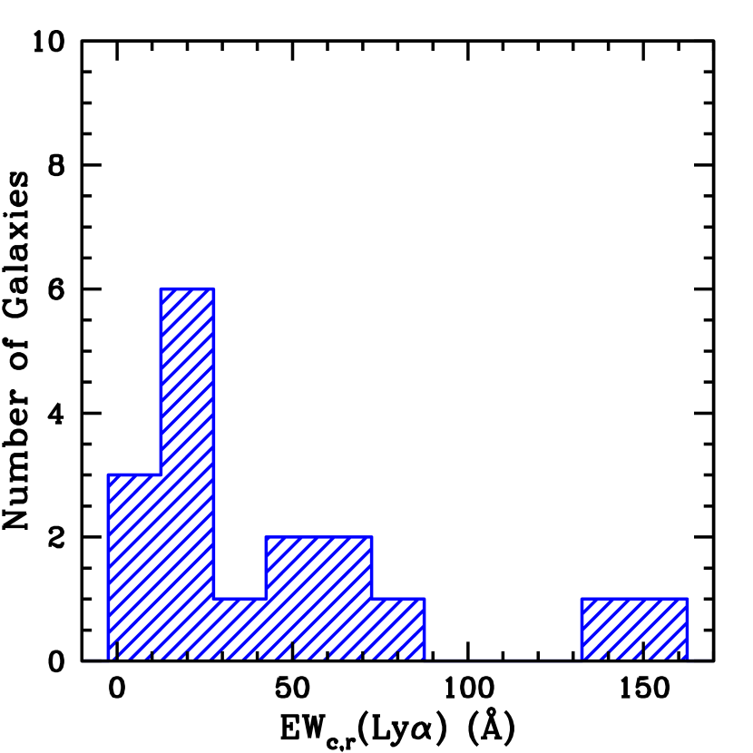
Figure 10.— The distribution of lower limits to the EW of the LAE candidates in our sample. Lower limits were calculated using line fluxes minimally corrected for slit losses and either the detected magnitude or the magnitude of the completeness limit in a filter completely redward of the Ly$\alpha$ emission (for $z<4.9$) or encompassing the Ly$\alpha$ emission (for $z\geq 4.9$).

Figure 10 shows the distribution of our EWs calculated from either the broadband magnitude completeness limit or the broadband magnitude of the detection redward of the Ly$\alpha$ line. The distribution is strongly skewed towards very modest values ($\sim$25 Å) of the EW as compared to measurements from other surveys (Dawson et al. 2004, H04, O08). This result is not surprising, due to the bulk of our sample populating the faint end of the Ly$\alpha$ luminosity function and to the manner in which we estimate the continuum luminosity of candidates undetected in the imaging data. Since the continuum luminosity is essentially independent of Ly$\alpha$ luminosity and since the estimated continuum luminosity is most likely significantly brighter than the true continuum luminosity of our candidates, the observed distribution may be more reflective of the way in which the EW was calculated rather than of any intrinsic properties of the LAE candidates. Still, the observed EW distribution is comparable to the results of the GLARE survey (Stanway et al. 2004, 2007), a comparably dim sample of LAEs, suggesting that there may be inherent properties of low-luminosity LAEs which contribute to our observed distribution.

4.3. Star-Formation Rates and Star-Formation Rate Density

For each LAE candidate the star formation rate (SFR) was calculated by:

$$SFR\,[M_{\odot}yr^{-1}]=9.5\times 10^{-43}\,L_{corr}(Ly\alpha),$$ (9)

where $L_{corr}(Ly\alpha)$ is the line luminosity based on the calculation in Section 2.4 and Equation 8. The constant of proportionality in Equation 9 is derived from the H$\alpha$ relation used in Kennicutt (1998) which assumes continuous star formation with a Salpeter IMF and the ratio of Ly$\alpha$ to H$\alpha$ photons calculated for Case B (high [$\tau$(Ly$\alpha$) $\sim 10^{4}$] optical depth) recombination (Brocklehurst 1971) for an electron temperature of $T_{e}=10000$K and solar abundance. This corrected SFR still represents a lower limit to the intrinsic SFR of the galaxy due to the unknown amount of slit loss and due to the fact that we do not correct for dust extinction. Tables 1 and 2 list the calculated SFRs for all 17 LAE candidates. The typical LAE candidate galaxy in our sample forms stars at a rate of 2-5 $\rm{M}_{\odot}$ yr^-1, on the low end of SFRs found in other samples.

As a consistency check, we also calculated SFRs from the rest-frame ultraviolet continuum for the three LAE candidates that had detectable continuum in bands redward of the Ly$\alpha$ line. In no cases was this measurement possible from the spectra as the continuum strength in the spectra redward of the Ly$\alpha$ line was not strong enough for a reliable measurement. Each of the UV SFRs were derived from the flux density of the three photometrically detected LAEs, measured from their F814W magnitudes and converted using the Madau et al. 1998 formula:

$$SFR_{UV}\,[M_{\odot}yr^{-1}]=L_{\nu,UV}/(8\times 10^{27}),$$ (10)

where L_ν,UV is a luminosity density calculated at $\sim$1500 Å. Since the three LAEs detected in the photometric data are at different redshifts, the effective rest-frame wavelength for the F814W filter changes slightly. However, we made no attempt to K-correct the observed flux densities as the effective rest-frame wavelength is always within 80 Å of 1500 Å and because the spectrum of LAEs are relatively flat in the UV. Table 2 lists the UV-derived SFR as well as the absolute UV magnitude for each of the three LAE candidates detected in the imaging data. The values of the SFR derived in this manner are very similar to the SFR derived from the Ly$\alpha$ line, with the exception of one of the candidates (FG1.20), suggesting that slit losses for two of these candidates is minimal (not surprising since one of the objects, 16XR1.72, was targeted).

Another quantity of interest for any population of high redshift galaxies is the star formation rate density (SFRD), which can be used to determine the onset of reionization in the universe. Observations of very high redshift ($z\gtrsim 6$) LAEs and LBGs (Malhotra & Rhoads 2004, hereafter MR04; Kashikawa et al. 2006, hereafter K06; Shimasaku et al. 2005; Taniguchi et al. 2005; Bouwens et al. 2003, 2004b, 2006; Bunker et al. 2004), Gunn-Peterson troughs in very high-redshift quasars (Becker et al. 2001; Djorgovski et al. 2001; Fan et al. 2006), and optical depth measurements from the Wilkinson Microwave Anisotropy Probe (WMAP; Spergel et al. 2007; Hinshaw et al. 2009) all suggest that the universe was reionized many 100s of Myrs prior to the observational epoch of our sample. The dominant population responsible for this reionization remains an open question. The evolution in the bulk contribution from LAEs has only recently been explored and shown to be a substantial contributor of ionizing flux from $z=3.1-5.7$ (O08; M08). However, such samples are only able to directly measure contributions from galaxies on the bright end of the luminosity function. The contribution from sub–$L_{\ast}$ LAEs are inferred by extrapolation of the best-fit luminosity function to faint Ly$\alpha$ line luminosities. Since many of our candidates lie far below the typical estimates for $L_{\ast}$ at these epochs, we can better characterize the contribution from such populations. It may be that galaxies with typical Ly$\alpha$ luminosities comparable to our sample ($\lesssim 0.1L_{\ast}-L_{\ast}$) represent the dominant contribution to the cosmic SFR amongst LAEs, a trend observed in $z$=2-5 LBG populations (Sawicki & Thompson 2006).

Using the entire survey volume and all our LAE candidates, we find an SFRD of $5.2_{-0.6}^{+1.0}$ $\times$ $10^{-3}$ ($4.5_{-0.6}^{+0.9}$ $\times$ $10^{-3}$ excluding Q=1 candidates) $\rm{M}_{\odot}$ yr^-1 $\rm{Mpc}^{-3}$. These values should be viewed as lower limits to the SFRD, as we make no corrections for added slit loss (due to the unknown position of the LAE candidate) or correction for extinction of Lyman continuum photons. Though dust corrections are important to determine the SFRD, this correction is perhaps not problematic if we are concerned only with the number of photons available to ionize the universe at these epochs as any Ly$\alpha$ photon that is absorbed by dust will make little or no contribution to the re-ionization of the universe. The errors should also be viewed as lower limits, as we do not incorporate formal errors due to cosmic variance, though we make some effort to quantify its effects (see Section 5.3). Despite these complications, a comparison the observed SFRDs of the Cl1604 LAE candidates gives values consistent with or exceeding the contributions of super-$L_{\ast}$ LAE galaxies found at $z$ = 5.7 (M08, O08), but significantly less than the contributions from $z=3-6$ LBGs ($\sim 1-2\times 10^{-2}$ $\rm{M}_{\odot}$ yr^-1 $\rm{Mpc}^{-3}$: Giavalisco et al. 2004; Bouwens et al. 2004a, 2006; Sawicki & Thompson 2006, Iwata et al. 2007). While some LBG surveys correct for contributions from galaxies dimmer than the completeness limit of the survey by integrating the observed luminosity function, we have made no such correction. Even though this correction could, in principle, be large enough to push our observed SFRD to levels competitive with LBG surveys, the faint-end of the LAE luminosity function is less constrained than the low luminosity end of the LBG luminosity function making extrapolation uncertain. If we assume that LAEs behave like LBGs at low luminosities, exhibiting relatively shallow faint-end slopes, the contributions from galaxies dimmer than the completeness limit of our survey ($\sim$0.1-0.2 $L_{\ast}$) would contribute only 10%-15% to the total SFRD at the redshifts of interest.

To quantify the evolution across the redshift range of our LAE candidates, we split our data into two redshift bins dictated by two OH transmission windows: (1) from $z=4.1$ (the onset of our spectral sensitivity) to $z=4.95$ (the onset of significant contamination from bright airglow lines, see Figure 1), and (2) between $z=5.6$ and $z=5.8$, an atmospheric transmission window used by many narrowband imaging surveys. These choices of bins exclude only one LAE candidate, 16XR1.97 at a redshift of $z=5.02$.

The first redshift bin contains 14 LAE candidates, 11 of which are high quality. The volume of the survey in this wavelength range, calculated in the same manner as in Section 2.2, is 4.99$\times 10^{3}$ $\rm{Mpc}^{3}$. The SFRD for the lower redshift sample is $\rm{SFRD}_{z\sim 4.55}$ = $12.1_{-1.7}^{+2.6}\times 10^{-3}$ ($11.1_{-1.7}^{+2.6}\times 10^{-3}$ excluding Q=1 candidates) $\rm{M}_{\odot}$ yr^-1 $\rm{Mpc}^{-3}$, a density rivaling the contribution of LBGs at this epoch. While this bin contains a large fraction of our LAE sample, any conclusions must be tentative, as cosmic variance can dramatically change the observed value (see Section 5.3).

The higher redshift bin contains two candidates (both high quality) within a survey volume of 1.44$\times 10^{3}$ $\rm{Mpc}^{3}$. The SFRD for the higher redshift sample is $\rm{SFRD}_{z\sim 5.7}$ = $4.4_{-1.1}^{+1.6}\times 10^{-3}$ $\rm{M}_{\odot}$ yr^-1 Mpc^-3, more consistent with the average SFRD of the survey and consistent within the errors of extrapolated SFRDs found by other surveys at similar redshifts (Rhoads et al. 2003, M08, O08). Since the high redshift bin contains only two LAE candidates, the measured value of the SFRD in this bin is highly susceptible to cosmic variance effects. While any conclusions that involve the high redshift bin are very uncertain, the drop in SFRD density at high redshift is a statistically significant effect and could possibly represent real evolution in the properties of LAEs as the observational epoch nears the epoch of re-ionization. If we instead choose to exclude the high redshift candidates from our sample and only use the lower redshift bin at $z\sim 4.55$, the observed SFRD is still significantly larger than those of higher redshift samples of LAEs (Rhoads et al. 2003; Ajiki et al. 2003; Shimasaku et al. 2006, hereafter S06; O08; M08). However, the derived SFRD at $z\sim 4.55$ is also quite a bit higher than some samples at comparable redshifts (Dawson et al. 2007, S08), suggesting that the observed change in SFRD from $z\sim 4.55$ to $z\sim 5.7$ probably arises through some combination of cosmic variance effects and real evolution in the LAE population. While marginally inconsistent with other measurements of the evolution of the LAE SFRD from $z\sim 4.55$ to $z\sim 6$ (O3; O8; Rhoads et al. 2003; Dawson et al. 2007), these results are consistent with the general evolution of the star-forming properties of LBG populations (Bouwens et al. 2004a; Sawicki & Thompson 2006; Yoshida et al. 2006; Iwata et al. 2007) and the overall picture of decreasing contribution to the cosmic SFRD from LAEs with increasing lookback time (Taniguchi et al. 2005).

4.4. Velocity Profiles

The observed line profile of the unsmoothed composite spectrum of the 13 high quality Ly$\alpha$ emitters was fit using a five parameter single Gaussian model similar to the model used in S08. In this model we assumed that the ISM absorbed all Ly$\alpha$ photons blueward of the centroid of an unattenuated Gaussian emission line, allowing us to produce the characteristic shape of the Ly$\alpha$ line. The mean wavelength of the original Ly$\alpha$ emission was allowed to freely vary, as our uncertainty in the redshift is coupled to our inability to quantify the extent of the absorption blueward of the Ly$\alpha$ line. Additionally the effective FWHM of our spectral setup, in principle a known quantity, was allowed to vary due to our ignorance of the placement of the LAE on the slit and the magnitude of the change in FWHM resolution as the LAE moves out of the slit. The background, dispersion, and amplitude of the Gaussian were also allowed to vary. This is, of course, a very simple model of the Ly$\alpha$ emission. In real galaxies there are typically multiple emission components offset in velocity space. In the case of LAEs, there can also be a significant excess of flux in the far red end of the line profile due to backscattering of Ly$\alpha$ photons by surrounding H II regions (S08; Westra et al. 2005). Still, this model allows us to gain some insight into the average properties of the main velocity component of our LAE candidates.

Figure 11 shows the best-fit model line profile overplotted on the co-added spectrum of the high quality LAEs. This simple model does reasonably well reproducing the observed line profile. It is interesting to note that if the model represents, even roughly, the intrinsic, unattenuated Ly$\alpha$ line, the truncation of the Ly$\alpha$ line by the IGM results in an attenuated line which is offset from the original line profile by nearly 100 km s^-1. The best-fit intrinsic velocity dispersion of 136 km s^-1 is marginally consistent with the findings of S08 and LAEs detected in some narrowband imaging surveys (H04) and is at the extreme low end of the mass function of other surveys (M08; Dawson et al. 2004).

There are two main discrepancies between the data and the simple truncated Gaussian model. The first is the failing of the model to reproduce flux just blueward of the centroid of the Ly$\alpha$ line at $\sim$ 1215 Å and again at $\sim$ 1214 Å. Such excesses could arise from a non-trivial amount of Ly$\alpha$ photons escaping attenuation from pockets of neutral hydrogen. Indeed, even at the highest redshifts of our Q=3 LAE candidates ($z\sim 5.6$), Equation 7 predicts an escape fraction ($f_{esc}$) of $\sim 5\%$, increasing to more than 40% at the lowest redshifts. The model also fails to produce enough flux at the extreme red end of the line, showing a moderately significant decrement in flux at $\sim$ 1217.5 Å as compared to the data. This unaccounted flux could be explained by backscattering of Ly$\alpha$ photons from galactic outflows as a result of star formation processes (Dawson et al. 2002; Mas-Hesse et al. 2003; Ahn 2004; Westra et al. 2005, 2006; Hansen & Oh 2006; K06). The offset between the observed flux excess and the centroid of the Ly$\alpha$ emission is $\sim$440 km s^-1, consistent with this interpretation and with measurements from other surveys (Dawson et al. 2002: 320 km s^-1; Westra et al. 2005: 405 km s^-1; S08: 420 km s^-1). It is interesting to note that these signatures appear in both the luminosity and uniform weighted stacked spectra, suggesting that such outflow processes are pervasive in low-mass high-redshift star-forming galaxies. However, both excesses are near the level of the noise in the co-added spectrum. While it is plausible to attribute these excesses to such astrophysical processes, more data are necessary to make any definitive conclusions. We, therefore, defer more complicated modeling of the composite emission line profile until all ORELSE fields are included.

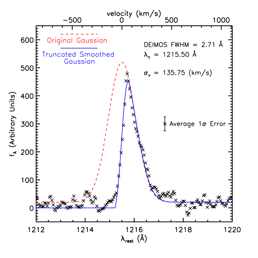
Figure 11.— A simple single Gaussian model fit to the unsmoothed composite (luminosity weighted) spectrum of high-quality (Q=2,3) LAE candidates. All flux blueward of the peak of the Gaussian has been removed in order to approximate the effects of attenuation from HI regions. The resultant profile is smoothed with a second Gaussian simulating instrumental broadening. The peak wavelength and width of the original Gaussian as well as the instrumental broadening are all free parameters in the model. The model profile fits the data extremely well, with a few notable exceptions.

5. Ly$\alpha$ Emitter Number Counts and Luminosity Functions

5.1. Number Counts and Cumulative Number Density

The depth of our data allows us to detect galaxies down to a limiting luminosity of $8.8\times 10^{41}$ ergs s^-1 over the entire redshift range of our survey and down to $3.7\times 10^{41}$ ergs s^-1 at $z=4.4$. This is almost a factor of 2 deeper than the recent spectroscopic survey of S08, previously the deepest survey for LAEs to date, and nearly a factor of 10 deeper than the completeness limits of recent narrowband imaging surveys (O08; Dawson et al. 2007; Murayama et al. 2007). Since our survey probes deeper in the luminosity function than previous surveys, any results that involve raw number counts of LAE candidates must be corrected for differing survey flux limits if proper comparisons are to be made.

One way to disentangle number counts from the effects of varying flux limits is to consider the cumulative number density of LAEs. Since the overall shape of the function should be identical, in the absence of cosmic variance and any instrumental effects, the galaxy populations from surveys of differing flux limits can be cast in a single functional form. Figure 12 shows both the cumulative number counts of all LAE candidates and of the highest quality (Q=3) LAE candidates in the Cl1604 field as compared to other surveys. Although the bulk of the candidates in the Cl1604 field reside at $z$ $<$ 5, the number counts lie above the measurements of surveys at similar redshifts. These number counts are also significantly higher than the lower limits of S08, a survey with a nearly identical instrumental setup to our own. Extrapolating down to the limiting luminosity of our survey, the Cl1604 LAE candidates seem to be instead broadly consistent with the number counts of LAE surveys at much higher redshifts.

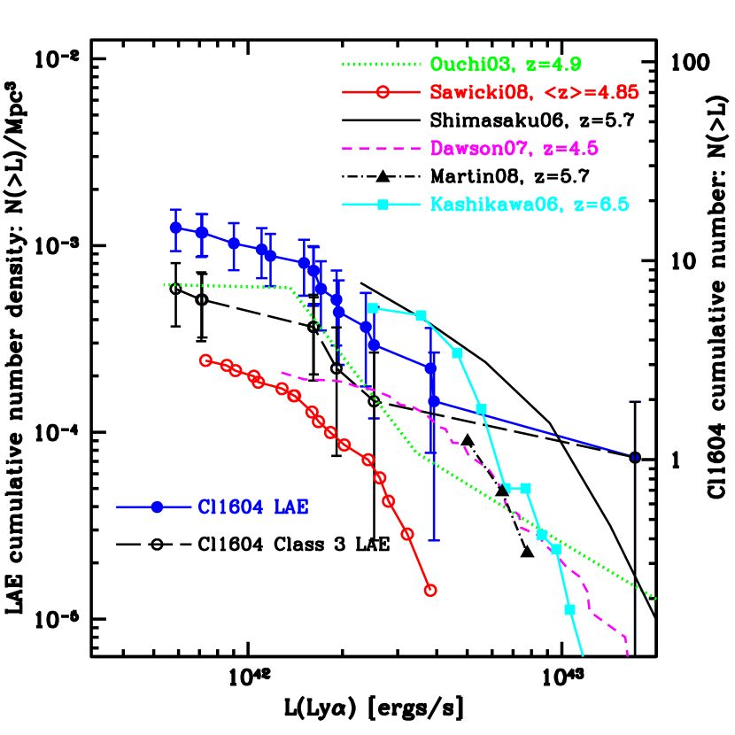
Figure 12.— Cumulative number density of LAEs detected in the Cl1604 field plotted as a function of Ly$\alpha$ line luminosity minimally corrected for slit losses ($\omega=0.8$; see Section 2.3). The right axis shows the cumulative number of LAE candidates detected in our survey. The observed number counts are more consistent with LAE populations at higher redshift ($z\geq 5.7$) than populations at more moderate redshifts ($z\leq 4.9$). Even excluding all but our highest quality (Q=3) candidates the number density is consistent with only the highest measurements of other surveys at similar redshifts. Error bars are derived from a combination of Monte Carlo simulations that incorporate the uncertainties in the luminosities (effectively which bin a given LAE candidate will fall in) and Poisson statistics, assuming (improperly, see Section 5.3) that LAEs have a spatial distribution reasonably similar to that of a Gaussian random field. Introducing formal measurements of uncertainties due to cosmic variance (not yet possible for this sample) will cause these errors to increase. Note that the S08 number counts plotted in this figure and Figure 14 differ from those plotted in S08 as we include LAEs detected at all redshifts in their survey (with the exception of two marginal candidates), whereas they only include LAEs detected between $z=4.2$ and $4.9$

There are many possible explanations for this discrepancy. While more exotic possibilities are discussed in Sections 5.4 and 5.5, there are simpler explanations which can be explored immediately. One possibility that would make our results slightly more consistent with other surveys at similar redshifts is the exclusion of the object 16XR1.72 (the LAE candidate at L_Lyα$\sim$1.7$\times$10⁴³ in Figure 12). This is an extremely bright ($\sim$2-3 L_∗) object that is unlikely to have been detected in a survey with our limited volume. Its presence is a strong indication that cosmic variance of such galaxies may have biased our results high for bright LAEs and its exclusion would serve to eliminate this effect at the brightest end of the cumulative number density distribution. Another possibility is the large uncertainties in the fluxes (luminosities) of the LAE candidates due to slit loss and flux calibration. As discussed in Section 2.3, the absolute flux calibration of the data was accurate to only 60%, further compounded by a possible systematic offset which underestimated the true value of the flux. Ignoring for the moment the systematic offset, the uncertainty in the flux calibration, combined with Poisson errors, could cause any given LAE candidate to shift nearly a factor of 2 in brightness (1$\sigma$) in either direction. Although significant, this shift would not change our conclusions, as our data would still be broadly consistent with the higher redshift surveys and broadly inconsistent with the moderate redshift surveys. Any systematic offset due to slit attenuation (see Section 2.3 for a full analysis) would cause an underestimate in the line flux and shift the cumulative number density curve to the right, only reinforcing our conclusions. If flux errors are the only potential contaminant in our results, our data suggest minimal evolution in the Ly$\alpha$ number density from $z=4.4$ to $z=6.5$. However, as we explore in the following two sections, there are other explanations which allow for evolution in the Ly$\alpha$ luminosity function.

5.2. Clustering of Ly$\alpha$ Emitters at $z\sim 4.4$ and $z\sim 4.83$

Since our survey encompasses an extremely small volume compared to other contemporary surveys, we are susceptible to sampling galaxies whose distributions are unrepresentative of the distributions observed in larger LAE surveys. Effects such as strong clustering of LAEs (O03) which lead to high levels of cosmic variance can play a large role in surveys with limited breadth. Similarly, variance in the observed number densities of LAE populations could be caused by inhomogeneities of intervening HI regions, as areas with a sparser density could manifest in increased detections of LAEs. While we will defer any complex treatment of cosmic variance until we can include all of the ORELSE fields, we attempt to quantify its effects in our survey in the following section. However, preliminary results from LAE searches in other ORELSE fields indicate similar detection frequencies, suggesting that cosmic variance may not be the sole cause of the large LAE number densities observed in the Cl1604 field relative to other $z\sim$5 surveys.

We do see significant evidence for clustering in our data, so it is possible that this clustering, combined with strong (Poissonian) sample variance, could be enough to explain the observed discrepancy in LAE number counts in the Cl1604 field relative to other surveys at the same redshift. As shown in Figure 7, there is a clear redshift peak at $z\sim 4.8$, as well as a less pronounced peak at $z\sim 4.4$. This is recast in Figure 13 where each LAE is plotted against the foreground of the supercluster, with the two redshift peaks being differentiated from the general LAE population.

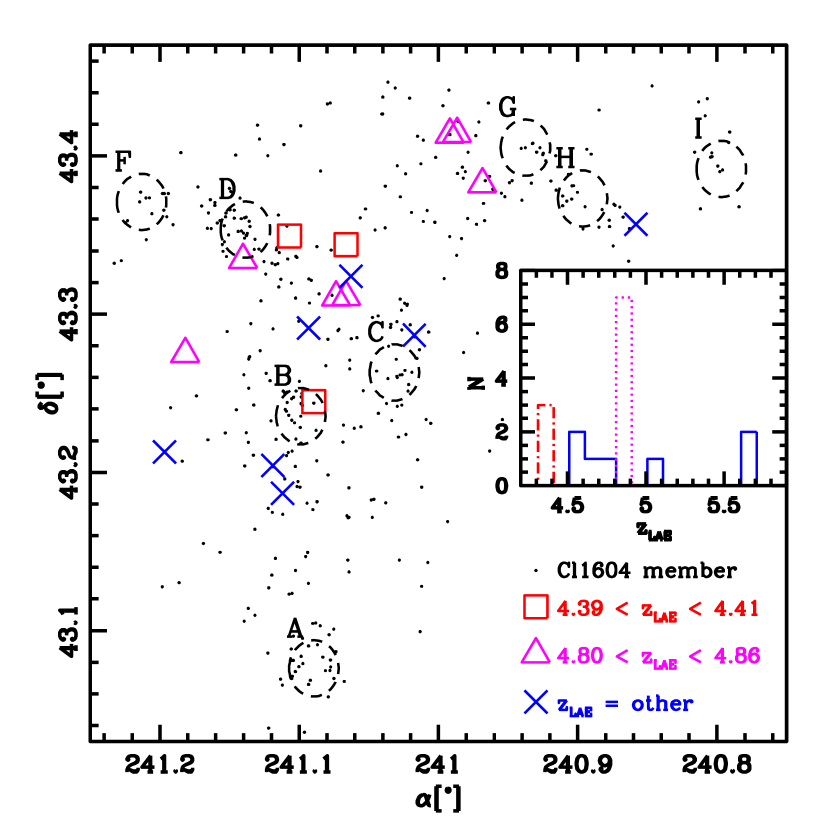
Figure 13.— The LAE candidates plotted against the foreground of the Cl1604 supercluster, with the two possible LAE structures at $z\sim 4.4$ and $z\sim 4.8$ shown as separate symbols. A redshift histogram of all LAE candidates (more finely gridded than the one in Figure 7) is shown to the right of the supercluster. For illustration, the name of each cluster as well as dashed circles that represent radii of 0.5 $\rm{h}^{-1}$ Mpc are overplotted. The dot-dashed and dotted lines in the histogram show the redshift distributions of the possible LAE structures at $z\sim 4.4$ and $z\sim 4.8$, respectively. The solid line shows the redshift distribution of the remaining “field” LAE candidates.

While the galaxies are not strongly clustered spatially, the observed distribution is broadly consistent with the spatial distributions and number densities of other structures found at high redshift (e.g., Shimasaku et al. 2003) and represents a significant overdensity when contrasted with normal “field” populations of LAEs. Using the coverage provided by the slits to calculate the survey volume at these redshifts, we recover a cumulative number density of $2.6\times 10^{-2}$ $\rm{Mpc^{-3}}$ and $1.4\times 10^{-2}$ $\rm{Mpc^{-3}}$ for the $z\sim 4.4$ and $z\sim 4.83$ structures, respectively, which are inconsistent at the $>$99.99% C.L. with field counts of LAEs (see Figure 14).

Since we have truncated the bounds of the data knowing the redshift range of the two structures involved, it is possible that we are overestimating the number density for these structures. However, in the absence of clustering we would expect our data to closely resemble the DEIMOS response function in areas absent of bright airglow lines. Since we are sensitive to a level far below typical estimates of $L_{\ast}$ across the entire redshift range of the survey, there should be little dependence of the number counts in our data on epoch. We are most sensitive to the redshift range 4.5-4.9 where the DEIMOS throughput is maximized, the airglow lines are minimal, and the full survey area is exposed to these wavelengths. It is surprising, therefore, that nearly all of our candidates in this redshift range lie in a narrow peak in redshift space, and that another peak exists outside the range of this area of high spectroscopic sensitivity.

If we exclude the LAEs in these two redshift peaks from our general LAE sample on the grounds that they belong to rare structures, we are left with a total of seven (six high quality) LAE candidates in our sample that represent a typical sampling of the LAE field populations. This reduction in the number of candidates drops our number counts to levels consistent with, but still higher than, other surveys at similar redshifts within the bounds of reasonable (Poissonian) sample variance (see Figure 14).

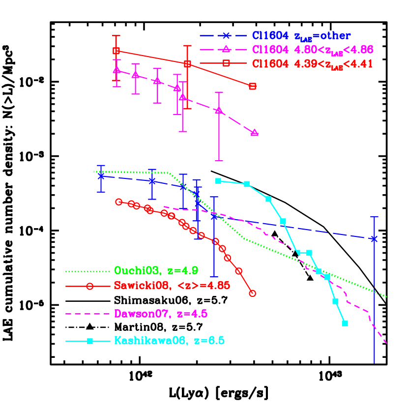
Figure 14.— The cumulative number density of LAEs as in Figure 12, but with the two possible LAE structures at $z\sim 4.4$ and $z\sim 4.8$ differentiated from the general population. The volume for each potential structure is bounded by the redshift range of the LAE candidates in the sample and calculated from the slit area exposed at those redshifts (wavelengths). The number densities of these potential structures are several orders of magnitude above field populations at all redshifts. If these structures are real, the number density of our remaining LAE candidates begin to be more consistent with moderate redshift ($z\leq 4.9$) LAE populations. Error bars are derived in the same way as Figure 12. Error bars in the last bins of the two LAE structure curves have been removed for clarity.

5.3. Cosmic Variance

Since the LAE candidates detected in the Cl1604 field represent one of the first detections of a reasonably large sample of faint LAEs, little is known about the clustering behavior of such galaxies. While the similar depth of the spectroscopic data in other ORELSE fields will allow for the study of statistical properties of faint LAE populations, the data presented in this paper is limited to one field. Thus, it is possible, given the clustering observed of brighter LAEs (O03; Shimasaku et al. 2003; S06), that our measurements of cumulative number densities (Section 5.1) or luminosity functions (Section 5.4) are biased by uneven sampling of the spatial distribution and the clumpiness of the population. As large statistical samples of faint LAEs do not exist, we must estimate by other means the likelihood that we would have detected the same number of LAE candidates if our survey had observed a different region of the cosmos.

In order to estimate this likelihood and to measure the magnitude of cosmic variance on the Cl1604 LAE candidates, simulations were run on four different samples of LAEs. The four fields were chosen because they contain a large number of LAEs, which were uniformly (or nearly uniformly) sampled over a large comoving volume and spanned the redshift range of the Cl1604 LAE candidates. The samples were: 1) the LALA spectroscopic sample in the Boötes field at $z\sim$4.5 (D07), 2) the Subaru Deep Field (SDF) at $z\sim$4.9 (O3; hereafter SDF+LSS), 3) the SDF at $z\sim$4.9, excluding the volume containing the large scale structure as defined in Shimasaku et al. (2003; hereafter SDF-LSS), and 4) the SDF at $z\sim$5.7 (S06; hereafter SDFhighz). The LAE candidates in all fields were selected using narrowband imaging methods and, in some cases, followed up with spectroscopy. Although each survey sampled a large volume ($\sim$1$\times$10⁶ Mpc³), their coverage was concentrated at nearly one epoch. However, since each survey has moderately large coverage in the transverse directions, the variance observed in each sample likely represents a reasonable estimate for the cosmic variance of brighter LAEs at that epoch. For simplicity, the transmission of the narrowband filter was assumed to be a top-hat response, with the hat size equal to the FWHM of the true filter response curve centered around the effective wavelength.

For each realization of the simulation in each field, an area was “observed” that would yield the survey volume of the Cl1604 spectral data (i.e. 1.365$\times$10⁴ Mpc³) given the filter setup. For the SDF samples, where LAE candidates were selected using only one narrowband filter, this area corresponded to roughly 65 arcmin². In the LALA field the area observed in each simulation was significantly less ($\sim 22$ arcmin²) due to the continuous coverage of their five narrowband filters, which span the line of sight direction from $z=4.37$ to $z=4.57$. The observation in each realization consisted of counting the number of LAEs detected in a continuous square area, whose central R.A. and decl. were determined by randomly drawing from a uniform distribution bounded by the spatial coverage of each survey. The results of these simulated observations are shown in Figure 15.

The results of each simulation are considerably different, suggesting that, even in surveys for LAEs that probe large comoving volumes, cosmic variance can play a large role or, alternatively, that the clustering statistics of LAEs evolve rapidly between $z\sim$4.5 and $z\sim$5.7. The variations may also arise from the difference in the parameters of each survey (e.g., limiting magnitude, completeness, purity). The results using the LALA sample in the Boötes field likely represents a lower limit to the cosmic variance and simulated LAE number counts because only 60% of LAE candidates selected by narrowband imaging were targeted by spectroscopy. Conversely, both the SDF+LSS and SDF-LSS samples have estimated purities of 60%-70% (O03). Thus, they represent an upper limit to the cosmic variance. The SDFhighz sample, which consists of a mix of spectroscopically confirmed LAEs and objects selected solely through narrowband imaging, falls somewhere in between the $z\sim 4.9$ SDF and the LALA sample in terms of completeness and purity.

In each panel of Figure 15, the two dashed lines mark the number of LAEs that we expect to observe in the Cl1604 field (i.e., 3) based on the extrapolating the number counts of surveys of LAEs at similar epochs (D07; S08) to the limiting luminosity of our data and the actual number of LAE candidates (i.e., 17) that we detect of all qualities. For both the LALA and SDFhighz fields, these simulations rule out cosmic variance as the sole cause of the observed excess of LAEs detected in the Cl1604 field at $>99.99$% C.L. However, since the bulk of our galaxies lie between $z$=4.4 and $z$=4.9, and since the LALA data are sparsely sampled, we focus on the results of the two SDF fields at $z\sim$4.9. In both cases, the observed number of LAEs detected in the Cl1604 are allowable within the bounds of the simulated cosmic variance. The likelihood of recovering at least 17 LAEs in the SDF+LSS simulations is 26% compared to only 6% in the SDF-LSS simulations. This result strongly supports the conclusion reached in $\S$5.2: we may be observing at least one large scale structure of LAEs in the Cl1604 field.

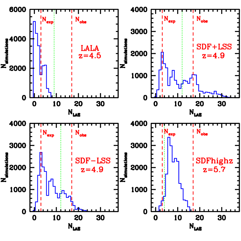
Figure 15.— Four different simulations of the effects of cosmic variance on the observations in the Cl1604 field. The four simulations are designed to cover a large range of redshifts and LAE samples. Each panel represents simulated observations of LAEs from different narrowband imaging surveys (see Section 5.3 for details on the surveys). A histogram of the number of LAEs recovered in each realization is plotted in each panel. The two dashed lines correspond to the number of LAEs expected in the Cl1604 data sampling an “average” field at $z\sim$5 (N_exp) and the number of actual detections (all qualities) of LAE candidates in the Cl1604 data (N_obs). The dotted line in each panel represent the number of LAEs that we would have detected in the Cl1604 field if we instead adopt the completeness limit of each survey. These results suggest that cosmic variance is a major contributor to the excess of LAEs described in $\S$5.1.

However, each LAE sample from which these simulations were drawn is, on average, significantly brighter than the Cl1604 LAE candidate population. The completeness limits of each survey are roughly 3-8 times brighter than that of the Cl1604 survey. Thus, many of the Cl1604 LAE candidates may not be detected in these surveys. In order to place a lower bound on the number of galaxies that would have been detected (assuming all of our LAE candidates were at the survey redshift), we cut the Cl1604 LAE candidate population at Ly$\alpha$ luminosities at or above the luminosity corresponding to the completeness limit of each survey. This number, plotted as a dotted line in each panel of Figure 15, is a lower limit since the luminosities calculated for the Cl1604 LAE candidates are lower limits. Since we are cutting at the completeness limit and not the limiting luminosity, the number of LAEs that would be detected by each survey had they observed the Cl1604 field and covered a volume equivalent to the Cl1604 survey volume lies somewhere between the dotted and the rightmost dashed line in each panel. Including this cut, we find that the hypothesis that our field contains a large-scale structure is still favored, though less strongly, as 44% of the simulations in the SDF+LSS field recover 12 or more LAEs (the number of Cl1604 LAE candidates above the O03 luminosity limit) compared to only 25% in the SDF-LSS field.

While it is unclear what adding in fainter LAEs to these simulations would do to the measurement of the cosmic variance, it has been observed that low-luminosity ($\sim$0.3-0.5L_∗) LAEs are less strongly clustered than brighter ($\gtrsim 0.5$L_∗) LAEs (O03). While this trend may not extrapolate down to the limiting luminosities of this survey or may be an effect unique to the SDF at $z\sim$4.9, the consequences of adding in the population may be limited and may even serve to dilute cosmic variance. While no definitive conclusions can be reached, the main result of these simulations is that cosmic variance may be solely responsible for the observed excess of LAE number density detected in the Cl1604 field. Determining how likely that is, however, is beyond the ability of these simulations.

5.4. Ly$\alpha$ Emitter Luminosity Function at $\langle z\rangle=4.85$

Because a large majority of our LAE candidates remain undetected in our imaging, these objects are equally likely to fall anywhere within the bounds of our slits or perhaps, depending on their brightness, outside the bounds of our slits. Without any way of recovering the true position of these objects, the slit loss correction must be approached statistically.

The statistical correction is made using the simulation code designed specifically for this purpose by Martin and Sawicki (see MS04 for a more detailed explanation). Briefly, for each realization the underlying galaxy population is simulated by setting the parameters $L_{\ast}$, $\Phi_{\ast}$, and $\alpha$, fully describing a unique instance of the underlying distribution characterized by the Schechter (1976) function:

$$\Phi(L)dL=\Phi_{\ast}\,\left(\frac{L}{L_{\ast}}\right)^{\alpha}\,exp\left(\frac{-L}{L_{\ast}}\right)\,\frac{dL}{L_{\ast}},$$ (11)

Data are then simulated for a grid of Schechter parameters for redshift slices of $\delta z=0.1$ running from central redshifts of $z=4.15$ to $z=6.35$ and multiplied by the area exposed to each redshift interval in our survey. The area exposed on the sky was also allowed to vary (in a known way) as a function of source flux and the seeing. Since brighter objects can fall further from the center of the slit (widthwise) and still be detected by our survey, the area of our survey at all redshift intervals increased with increasing LAE flux. The range of simulated LAE luminosities for each redshift bin was left unbounded on the bright end and truncated on the faint end by an LAE luminosity that would result in a flux of $1.9\times 10^{-18}$ ergs s^-1 cm^-2 (ranging from $L($Ly$\alpha)=3.2\times 10^{41}$ ergs s^-1 at $z=4.15$ to $L($Ly$\alpha)=8.9\times 10^{41}$ ergs s^-1 at $z=6.45$). For every set of Schechter parameters, each simulated galaxy is “observed” by calculating the slit attenuation based on simulated slit losses for an unresolved source galaxy at a regularly sampled grid of positions with respect to the slit in 0.9$\arcsec$ seeing. The total number of LAE galaxies of all fluxes (luminosities) for that set of Schechter parameters is then recorded. Though we only include galaxies in these simulations with fluxes greater than or equal to the completeness limit calculated in Section 2.5, this choice results in conservative values of the Schechter parameters. Specifically, we underestimate the “true” Schechter parameters since the actual completeness limit of our survey is brighter than the limit calculated in Section 2.5 (due to the unknown amount of slit losses). Therefore, it is likely that the faintest galaxies in this simulation were not detected in our survey. Thus, this choice results in more simulated galaxies than if we had attempted to make a correction for slit losses, requiring us to observe more galaxies in the Cl1604 field to recover the same set of Schechter parameters.

From this simulation we are not able to recover a unique set of Schechter parameters due to our ignorance of how many genuine LAE galaxies are in our data. Furthermore, since the simulations allow each LAE candidate to have a range of Ly$\alpha$ luminosities, we are not definitively setting the number of galaxies detected at any given luminosity. This constraint would be essential if we were calculating specific values of $\Phi_{\ast}$ and L_∗. Instead, we can only limit the range of Schechter parameters by bounding the number of simulated galaxies for a given $\Phi_{\ast}L_{\ast}$ by the total number of genuine LAE galaxies in our data. It seems reasonable that the number of galaxies observed in the simulation be equal to at least 13, the number of high quality LAE candidates in our sample. However, this number does not represent a hard lower bound, as any real clustering in the data would not be accounted for in these simulations. Instead we set the lower bound as seven (six high quality) galaxies, the number of LAE candidates that exist outside the two possible structures and constitute a lower limit on our LAE field population.

The upper bound for this simulation is more ambiguous. The primary consideration is the nature of our completeness limit, the flux at which galaxies were cut in the simulation. We estimate that at our flux limit we do not miss more than two-thirds of the actual number of LAE galaxies in our data. Taking the 17 LAE candidates of all qualities as the upper bound on actual detections, this sets an upper bound for our simulations at 51 LAEs.

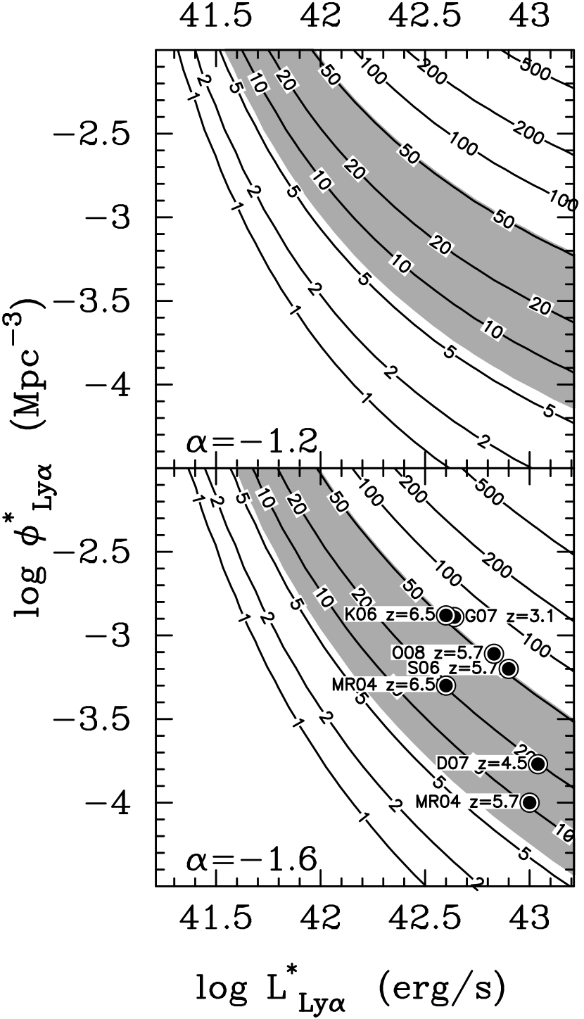
Figure 16.— The range of possible Schechter parameters, $\Phi_{\ast}$ and $L_{\ast}$, for simulated populations of LAEs approximating those observed in the Cl1604 field for two different faint-end slopes ($\alpha=-1.2$, top panel; $\alpha=-1.6$, bottom panel). The data are simulated assuming a completeness limit of $1.9\times 10^{-18}$ ergs s^-1 and is corrected for statistical flux losses. Each contour through the $\Phi_{\ast}L_{\ast}$ phase space represents the expected number of LAEs, given our instrumental setup and observing conditions, that should be detected in our data. The shaded contour shows the phase space allowed by our LAE candidates. For comparison the values of $\Phi_{\ast}$ and $\L_{\ast}$ are shown for different surveys that used similar values of the faint-end slope. (MR04: Malhotra & Rhoads 2004; K06: Kashikawa et al. 2006; S06: Shimasaku et al. 2006; D07: Dawson et al. 2007; G07: Gronwall et al. 2007; O08: Ouchi 2008)

For each panel in Figure 16 the shaded area represents the values of the Schechter parameters, the normalization ($\Phi_{\ast}$) and the characteristic luminosity ($L_{\ast}$) allowed by our data for the range of possible LAE galaxies detected by our survey. This analysis is done for two different faint end slopes, $\alpha$=-1.2 and $\alpha$=-1.6. Even if we knew the true number of LAEs in our data, due to the nature of the Schechter formalism and the sparseness of our data, we are not able to definitively determine unique values of the Schechter parameters from our simulations. However, our data does allow us to constrain the product, $\Phi_{\ast}L_{\ast}$, by the range bounded by the shaded area in Figure 16. Defining the best-fit Schechter product as the average value of $\Phi_{\ast}$$L_{\ast}$ for which we observe exactly 13 LAEs in the simulation and the range of possible $\Phi_{\ast}$$L_{\ast}$ values as the average of those which recover seven simulated LAEs (on the low end) and 51 simulated LAEs (on the high end), we find a best-fit Schechter product of $\Phi_{\ast}L_{\ast}=2.2^{+3.9}_{-1.3}\times 10^{39}$ ergs s^-1 Mpc^-3 for a faint-end slope of $\alpha=-1.6$.

As shown in Figure 16, our observed range in $\Phi_{\ast}$ and $L_{\ast}$ is consistent with measurements made by D07, O03, and MR04 and slightly low when compared to measurements made by K06, S06, G07, and O08. Although there is considerable variation in the measured values of $\Phi_{\ast}$ and $L_{\ast}$ even at similar redshifts, the comparisons of the Schechter parameters seem inconsistent with the comparisons in Section 5.1, in which the cumulative number density of the Cl1604 LAE candidates were more similar to the extrapolated number counts of higher redshift surveys (K06, S06) than surveys at lower redshift (e.g., D07). It is possible that our conservative estimates of both the number and luminosity of our candidate LAEs may be the source of this discrepancy rather than any real evolution in the luminosity function of Ly$\alpha$ emitters from $z\sim 4.85$ to $z\sim 6$. Since the choice of a faint-end cutoff can severely affect simulated numbers of LAEs, especially for steeper faint-end slopes, our choice of a simulated flux limit of $1.9\times 10^{-18}$ ergs s^-1 cm^-2 could have biased our results to lower values of $\Phi_{\ast}L_{\ast}$. To estimate the magnitude of this effect we ran the simulation again on a small portion of the data ($z=4.1$ to $z=4.9$) with a brighter completeness limit of $3\times 10^{-18}$ ergs s^-1 cm^-2. The recovered Schechter product was on average higher by a factor of $\sim$ 2, corresponding to a $\Phi_{\ast}L_{\ast}\approx 5\times 10^{39}$ ergs s^-1 Mpc^-3 for a faint-end slope of $\alpha=-1.6$, essentially pushing the contours up and to the right in both panels in Figure 16, encompassing the $\Phi_{\ast}L_{\ast}$ products of the other surveys within our range of allowed values. Since the true completeness limit of the Cl1604 spectral data is somewhat uncertain (see Section 2) and since the results of these simulations are extremely sensitive to the choice of this limit, we are not able to distinguish between the luminosity function properties of our sample and other samples of LAEs. Instead, we conclude that the Schechter parameters for the Cl1604 LAE population are broadly consistent with other measured values from $z\sim 4$ to $z\sim 6$.

5.5. Weak Lensing Contributions to the Luminosity Function

The Cl1604 supercluster is the most well-studied large-scale structure at high redshift. While no single cluster in the structure would be considered at the high end of the cluster mass function (Poggianti et al. 2006, 2008; Milvang-Jensen et al. 2008; Hamana et al. 2008), with the possible exceptions of cluster A ($\sigma_{v}$ $\sim$ 703 km s^-1) and cluster B ($\sigma$ $\sim$ 800 km s^-1) (G08), the large number of moderately massive constituent clusters and the structure’s large spatial extent make it an efficient astrophysical lens. The nature of the source population also lends itself to a large lensing effect: the lensing efficiency for LAEs being a monotonically increasing function of redshift for $z_{Ly\alpha}>z_{lens}$. The presence of this massive lens along with the high lensing efficiency for high redshift LAEs makes it necessary to properly account for lensing processes and determine whether such processes may explain the observed excess in number density counts over comparable field studies (see Section 5.1).

We consider the effects of strong and weak gravitational lensing separately, with strong gravitational lensing effects discussed in Section 5.5. The observational weak lensing effect considered here is a magnification of the source population due to the lensing-induced increase in observed surface area while keeping surface brightness constant. Assuming the slit is sufficiently large (or equivalently the galaxy is sufficiently small) to encompass this increased surface area, this magnification increases the brightness of observed objects and the frequency of detection by: (1) by lensing objects into the slit which were not already within the detectable area of the slit and (2) by increasing the total flux of galaxies that were just below the detection limit of the survey. Weak gravitational lensing could then increase both the overall normalization, $\Phi_{\ast}$, and the characteristic luminosity, L_∗, of the LAE luminosity function. These effects are opposite those of all other analyses and measurement techniques used in this study, which are intentionally designed and implemented to underestimate the line flux. Such effects, if significant compared to the other associated uncertainties in our measurements, could significantly alter our conclusions.

In principle, the most accurate approach to quantify the weak lensing effect would be to correct each LAE for the lensing-induced magnification. However, much more spectroscopy in the field (or other similar data) would be necessary to accurately measure the effect of weak lensing on each LAE. While a formal weak lensing analysis has been done on a small subsection of the field around cluster A (Margoniner et al. 2005) and will be done again with newly obtained ACS data (Lagattuta et al. 2010), the current data require us to take a more general approach. In order to simulate the effect of weak lensing, the eight clusters that comprise the Cl1604 supercluster were modeled by singular isothermal spheres (SIS) of the form:

$$\rho(r)=\frac{\sigma_{v}^{2}}{2\pi Gr^{2}},$$ (12)

While this model is an oversimplification of the true cluster mass profile, an SIS was used in place of a Navarro-Frenk-White (NFW, Navarro et al. 1996) profile because of the closed analytic form of the convergence and magnification solution. More importantly, however, since some of the clusters in Cl1604 are poorly sampled by spectroscopy (clusters F, G, H, I, and J), we were unable to constrain the characteristic radius, $r_{s}$, and the concentration parameter, $c$, needed to properly characterize an NFW profile.

Each cluster profile was simulated using velocity dispersions published in Gal et al. (2008) and central positions determined from the velocity and spatial centroids of the constituent cluster members. A velocity dispersion derived from cluster members within 1 $h^{-1}$ Mpc was adopted, chosen over 0.5 $h^{-1}$ Mpc or 1.5 $h^{-1}$ Mpc because it is the largest velocity dispersion that is relatively free from significant contamination from other clusters. Since $\rho$ scales as $\sigma^{2}$, this choice will allow us to measure the maximum possible (model dependent) lensing effect on the LAE population by the clusters.

For each realization of the simulation, new velocity dispersions were generated for each cluster by a Gaussian sampling of the published 1 $h^{-1}$ Mpc velocity dispersion errors. Thus, the velocity dispersion of the $i$th cluster was given by:

$$\sigma_{v,i}=\sigma_{i,1Mpc}+n_{i},$$ (13)

where $n_{i}$ is sampled from a Gaussian distribution with width equal to the velocity dispersion errors. This new velocity dispersion, along with the static central positions of each cluster, completely dictated the mass map for the field of each realization; any effects from substructure, other structures along the line of sight, or lensing due to individual cluster galaxies were completely ignored. The source plane was created by averaging the $z=3.7$ and $z=5.7$ field LAE luminosity functions taken from the large sample from the SXDS (O08), as our survey marginalizes over any evolution in the LAE luminosity function. The resulting Schechter function is parameterized by $\Phi_{\ast}=5.55\times 10^{-4}$ Mpc^-3, $L_{\ast}=8.5\times 10^{42}$, with a faint end slope of $\alpha=-1.5$. The source population was drawn from discrete luminosity bins of width 0.1 dex, which were evenly spaced between L $\sim$ $10^{41}$ $L_{\odot}$ and L $\sim$ $10^{43}$ $L_{\odot}$. These limits were chosen to span the entire observable range of luminosities in various surveys. The number of galaxies in each luminosity bin was given by:

$$N_{i}=\int_{L_{i}}^{L_{i+1}}\Gamma\,\Phi_{\ast}\,\left(\frac{L}{L_{\ast}}\right)^{\alpha}exp\left(\frac{-L}{L_{\ast}}\right)\frac{dL}{L_{\ast}},$$ (14)

where $\Gamma$ is the simulation volume of $3.85\times 10^{6}$ Mpc³. All galaxies in each bin were assigned the average luminosity in that bin, dictated by the bounds of the integration. Next, each galaxy was assigned a R.A. ($\alpha$) and decl. ($\delta$), generated randomly from the area bounded by (but not necessarily sampled by) the spectral coverage of the survey. In addition, a redshift was assigned to each source galaxy, drawn in a uniform random manner in the redshift range $z=4.4$ to $z=6.5$. In principle, we could have made the simulation more realistic by introducing evolution in the LAE population by using Schechter parameters based on various surveys at various redshifts. However, since the difference between the lensed and unlensed populations is relatively insensitive to our choice of Schechter parameters, we ignore this effect.

Once the $\sim$ 25000 generated LAEs were assigned unique redshifts, coordinates, and luminosities, each luminosity was converted into an observed flux using the luminosity distance of each LAE. With the source plane and lens plane completely constructed, the lensing formalism could then be applied. For the SIS profile the shear and convergence are equivalent, given for the $i$th LAE as:

$$\gamma_{i,j}=\kappa_{i,j}=0.9\left(\frac{\sigma_{j,new}}{250}\right)^{2}\frac{D_{ls,i,j}}{D_{s,i}\,\theta_{i,j}},$$ (15)

where the $j$th index represents the induced shear or convergence from the $j$th cluster in Cl1604 and $\theta$ is the angular separation of the $i$th LAE from the $j$th cluster in arcseconds. The magnification of the $i$th LAE is then calculated by:

$$\mu_{i}=\frac{1}{\left(1-\kappa^{2}\right)-\gamma^{2}}=\frac{1}{1-2\kappa},$$ (16)

The flux of each LAE was then increased by its respective magnification. A flux limit of $1\times 10^{18}$ ergs s^-1 cm^-2, reasonably approximating the flux limit of our survey, was imposed on both the original, unlensed source population and the newly generated weakly lensed population. The lensed flux was re-converted to an apparent luminosity, with the resulting observed populations shown in Figure 17.

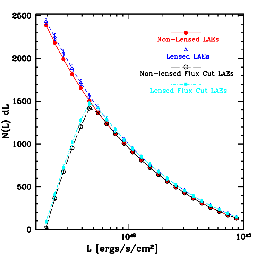
Figure 17.— Observations of simulated populations of LAEs in the absence of any lensing effects (solid lines) and after being weakly lensed by the Cl1604 supercluster (dashed lines). The two sets of curves show the differential number as a function of Ly$\alpha$ line luminosity prior to the flux cut (continuous and short dashed lines) and subsequent to the flux cut (long dashed and dot-dashed lines). For all line luminosities the weak lensing number counts are consistent with the unlensed population within 3$\sigma$. The biggest difference between the number counts ($\sim$10%) occurs at the line luminosity corresponding to the flux limit of $1\times 10^{-18}$ ergs s^-1 cm^-2 and dropping to negligible differences (1-2%) at higher luminosities.

The results conclusively demonstrate that the cluster-induced weak lensing effect is far too small to account for our increased number counts. The ensemble average increase in total detections from the unlensed to the lensed data is 6%, an effect which is consistent with unlensed number counts at the 2$\sigma$ level in most of the bins. The effect is small regardless of the luminosity of the lensed galaxy, with an average increase in number counts in each bin ranging between 2% for the brightest simulated galaxies and 8% near the characteristic luminosity, $L_{\ast}$.

Another way to quantify the magnitude of this effect is by the overall increase in the Schechter parameters $\phi_{\ast}$ and $L_{\ast}$. While not intuitively obvious as a measurement in the overall increase (or decrease) in the number counts of LAEs at different luminosities, it will give us some insight into possible systematic errors (as a result of unquantified weak lensing effects) in our final luminosity function parameters. A Schechter parameter model with a fixed faint end slope ($\alpha=-1.5$) was fit to both the unlensed and lensed data using a $\chi^{2}$ minimization routine. As the two Schechter parameters, $\Phi_{\ast}$ and $L_{\ast}$, are degenerate with one another (increasing $L_{\ast}$ necessitates a decrease in the normalization in order to maintain constant numbers of galaxies), the quantity of interest in these fits is not the individual parameters but rather the product $\Phi_{\ast}L_{\ast}$. For the unlensed data the best-fit parameters resulted in a $\Phi_{\ast}L{\ast}=4.0\times 10^{39}\pm 2.5\times 10^{38}$, differing from the product of the original input Schechter parameters due to the way the simulation is coarsely binned. Errors were calculated from the covariance matrix and the difference between the input and measured Schechter parameters. The fit to the lensed data resulted in a $\Phi_{\ast}L_{\ast}=4.3\times 10^{39}\pm 3.1\times 10^{38}$, representing an overall increase of 7.5%, but also consistent within the errors to the unlensed measurements. While a correction of this magnitude might be important for precision measurements, the other uncertainties in our data (e.g., flux calibration or flux losses due to the slit) far outweigh any induced weak lensing signal.

5.6. Strong Lensing Contributions to the Luminosity Function

When a galaxy is strongly lensed, either by the cluster potential or by a massive foreground galaxy, multiple images of the background galaxy are created on the sky. Depending on the relative positions of the lensing potential and the source (background) galaxy as observed projected on the sky, the resulting images of the original galaxy can be either fainter or brighter than the original galaxy, thus changing the observed luminosity function. This effect can also serve to push galaxies that would otherwise be too faint to detect above the flux detection limit, an effect which has been exploited by several surveys attempting to detect galaxies at very high redshift ($z$ = 6-10, Santos et al. 2004; Egami et al. 2005; Stark et al. 2007; Richard et al. 2009). It is also possible, though very unlikely, that the slit geometry is perfectly oriented to observe multiple images of the source galaxy, effectively increasing the frequency of LAE detections. While these effects may introduce severe bias when they occur, strong gravitational lensing has a comparatively small cross section, allowing us to explore the possible effect on the LAE candidate population in a much more direct way than the exploration of similar effects caused by weak gravitational lensing.

For an SIS lens multiple images form only for galaxies that lie within the Einstein radius ($\theta_{E}$). All of the LAE candidates lie very safely outside of any reasonable estimate of the cluster strong lensing regime (see Figure 18), meaning any cluster-induced lensing effects would be accounted for in the previous section’s analysis. The galaxy that comes closest to being strongly lensed is 16XR1.26, which falls greater than $3\theta_{E}$ outside of cluster B. While the true mass profile may differ from SIS and the cluster mass may be underestimated due to our choice of velocity dispersions, it is unlikely that either of these effects would be strong enough to increase $\theta_{E}$ to encompass 16XR1.26.

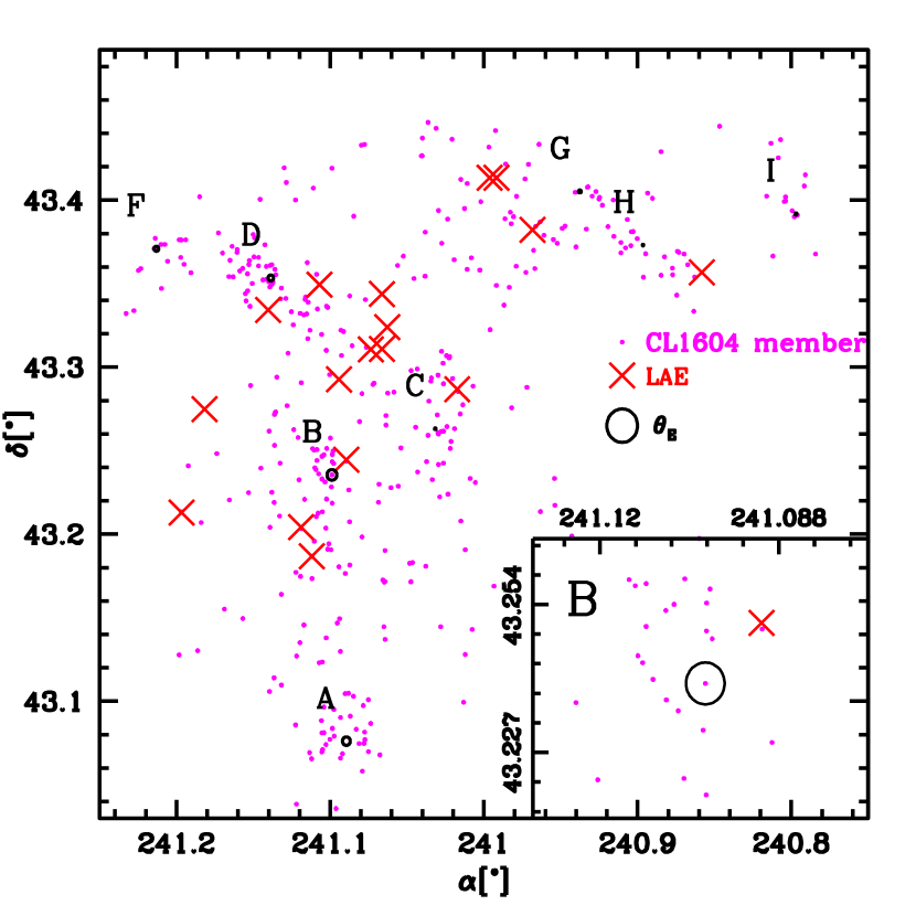
Figure 18.— LAEs with cluster members plotted with cluster Einstein ring radii ($\theta_{E}$), which characterizes the onset of the strong lensing regime. Einstein radii were calculated using an SIS profile, with velocity dispersions derived from all members within 1 $h^{-1}$ Mpc of the cluster center. All LAEs fall clearly outside the bounds of the cluster-galaxy strong lensing regime. The galaxy closest to any cluster Einstein radius is shown in the bottom panel, lying many Einstein ring radii outside the center of cluster B.

Another issue that should be considered when discussing strong lensing of the LAE candidate population is any strong lensing due to individual foreground galaxies. This search has, by definition, a foreground galaxy companion, typically quite massive, targeted by the spectroscopy. Since this galaxy lies within the length of the small DEIMOS slit, it is possible that this effect could be significant. In some cases there is an additional serendipitous detection of a foreground galaxy on the slit which further complicates the matter. However, there are two reasons why we can ignore this effect. The Einstein radius for an $L_{\ast}$ galaxy is of the order of 1$\arcsec$. While this value will change based on the mass of the spectroscopic target (or other foreground serendip) and the relative redshifts of the foreground galaxy and the LAE, it is a reasonable estimate of where the strong lensing effect might be significant. All of our highest quality (Q=3) LAE candidates lie outside the bounds of this cutoff; any galaxy that is considered to be highly likely to be a LAE but is within a 1$\arcsec$ radius of either the target or a foreground serendipitously detected galaxy is demoted to a lower confidence class (Q=2). Even considering only Q=3 LAE candidate galaxies, the detection frequency in our survey is significantly higher than most other surveys at the redshift of our sample, an effect which cannot possibly be attributed to lensing. Furthermore, even if there are galaxy-galaxy lensing effects for which this analysis has failed to account, our sample set is selected nearly identically to the LAE population detected in S08, with the possible exception that the spectroscopic targets in the Cl1604 field may be slightly more massive than those targeted by the DEEP2 survey. As they do not see similar excesses in their data it is likely that our observed excess comes from some combination of real, inherent properties of the observed LAE population, such as those discussed in the previous sections, and cosmic variance effects and cannot be attributed solely to lensing effects.

6. Summary

In this paper we have described a search for LAE galaxies in the 3.214 arcmin² ORELSE spectroscopic database in the Cl1604 supercluster field. In total, 17 high redshift candidate galaxies were found in a volume of $1.365\times 10^{4}$ Mpc³, with 13 galaxies meeting our high quality criteria. The redshifts of our LAE candidates ranged from $z=4.39$ to $z=5.67$. Many of our candidate galaxies ($\sim$90%) are dim compared to the typical characteristic luminosity at $z\sim 5$, with Ly$\alpha$ line luminosities ranging from 5.9$\times$10⁴¹ erg s^-1 ($\sim 0.1L_{\ast}$) to 1.7$\times$10⁴³ erg s^-1 ($\sim 2L_{\ast}$). We have contrasted our LAE candidates with a population of known low redshift single-emission line interlopers and blended [OII] emitters at intermediate redshifts. Our 13 high quality candidates have properties that differ significantly from the interloper population, giving us confidence in these objects as genuine LAE galaxies. The four lower quality objects do not distinguish themselves as well from the interloper population, implying that these galaxies probably represent a mixture of LAEs and lower redshift objects. The increased frequency in LAE detections compared to other surveys demonstrates the effectiveness of LAE searches that probe deep into the luminosity function rather than covering large comoving volumes. Our main results are as follows:

Lower limits on the Ly$\alpha$ EW have been derived for all of our LAE candidate galaxies, finding a distribution peaking at EW(Ly$\alpha$)$\sim$20 Å, similar to other low luminosity galaxies at high redshift. We have also derived a lower limit to the SFRs of our LAE candidate, finding that they typically form stars at a rate of 2-5 $M_{\odot}$ yr^-1.

From the entirety of our sample we determine an SFRD of $4.5_{-0.6}^{+0.9}$ $\times$ $10^{-3}$ $\rm{M}_{\odot}$ $\rm{yr}^{-1}$ $\rm{Mpc}^{-3}$. This density is similar to or exceeding the contribution from super-L_∗ LAE galaxies found at comparable redshifts, suggesting that sub-L_∗ LAEs play an important role in keeping the universe ionized at $z\sim 5$. Grouping our LAE candidates into low redshift ($4.1\leq z\leq 4.95$) and high redshift ($5.6\leq z\leq 5.8$) bins, we find moderate evidence for negative evolution in the SFRD. We measure an SFRD of $11.1_{-1.7}^{+2.6}\times 10^{-3}$ at $z\sim 4.65$ $\rm{M}_{\odot}$ $\rm{yr}^{-1}$ $\rm{Mpc}^{-3}$ decreasing to $4.4_{-1.1}^{+1.6}\times 10^{-3}$ $\rm{M}_{\odot}$ $\rm{yr}^{-1}$ $\rm{Mpc}^{-3}$ at $z\sim 5.7$, though our highest redshift bin contains only two galaxies making any conclusions about the evolution of the LAE SFRD tentative. The derived SFRD of LAEs at $z\sim 4.55$ is nearly equivalent to contributions of LBGs at similar redshifts, though this number is also strongly subject to cosmic variance effects.

A simple truncated Gaussian model was fit to the composite spectrum of our high quality LAE candidates. The best-fit velocity dispersion was 136 km s^-1, suggesting that our galaxies lie at the low end of the observed LAE mass distribution. While the model fits reasonably well, there were two noticeable discrepancies for which the model failed to account. First, we found modest evidence for excess light at 1214 Å and 1215 Å, which we tentatively attributed to a non-trivial Ly$\alpha$ escape fraction. There was also an observed excess at 1217.5 Å that may be the result of galactic outflows separated from the LAE candidates by 440 km s^-1. As this composite represents the average properties of our LAE candidates, this observed excess implies that outflow processes may be prevalent in low mass star-forming galaxies at high redshift.

We find the density of LAEs to be $\sim$1.5$\times 10^{-3}$ Mpc^-3 for $L$(Ly$\alpha$)$\gtrsim 6\times 10^{41}$ ergs s^-1, a frequency far higher than any other search for LAEs at comparable redshifts. We find that the excess is instead consistent with extrapolated cumulative number densities of higher ($z>5.7$) LAE surveys, initially suggesting minimal evolution in the LAE number density between $z=4.8$ and $z=5.7$.

We report on the possible discovery of two structures at $z\sim 4.4$ (three members) and $z\sim 4.8$ (seven members). Removing these galaxies from our sample and adopting the remaining galaxies as “field” LAEs, we find number densities consistent with lower redshift ($z\sim 4.5$) surveys, allowing for evolution in the LAE number density.

We investigate the effect of cosmic variance using simulated observations of four samples of narrowband-imaging-selected LAEs. The results of these simulations suggest that we cannot not rule out cosmic variance as the sole cause for the observed excess in the LAE density in the Cl1604 field. The results of the simulations also suggest that our field contains a large scale structure of LAEs, consistent with the observed redshift clustering of the Cl1604 LAE candidates.

Best-fit Schechter parameters were determined by simulating the effect of observing LAEs with our instrumental setup to account for unknown slit attenuation. The resultant best-fit Schechter product ($\Phi_{\ast}L_{\ast}$) was found to be $\Phi_{\ast}L_{\ast}=2.2^{+3.9}_{-1.3}\times 10^{39}$ ergs s^-1 Mpc^-3. Although these simulations are sensitive to the assumed completeness limit of the survey, we find that our results are generally consistent with other surveys both at intermediate ($z\sim 4.5$) and high ($z\sim 6$) redshifts.

Simulating the weak lensing effect induced by the Cl1604 supercluster using SIS models characterized by published cluster velocity dispersions, we find an average increase of 6% in the observed number counts (or equivalently luminosity) of simulated LAE populations between $z=4.4$ and $z=6.5$ as compared to unlensed populations. The observed change in the best-fit product of the luminosity function parameters ($\Phi_{\ast}L{\ast}$) due to weak lensing was 7.5%, consistent within the errors to the unlensed values, and far too small to explain our observed number density excess. We also investigated the effects of strong lensing induced by the supercluster, finding that no galaxies are likely strongly lensed by the cluster potential.

We thank Evan Kirby and Jeffrey Newman for useful discussions on coaddition techniques and for kindly providing their codes and Nick Konidaris for helpful advice and guidance with DEIMOS flux calibration. We thank Raja Guhathakurta for the idea. D.J.L. and B.C.L. thank Matt Auger for useful discussions and criticisms. We also thank the anonymous referee for useful comments and suggestions. B.C.L. wishes to thank Eric Opland and Carl Olding for making this work possible. B.C.L. also wishes to thank Margaret Thompson for careful reading of the paper and for the many grammar corrections: appear up here! This material is based upon work supported by the National Aeronautics and Space Administration under Award NNG05GC34ZG for the Long Term Space Astrophysics Program. The research of M.S. is financially supported by the Natural Science and Engineering Research Council of Canada and the Canadian Space Agency. Based in part on data collected at Subaru Telescope and obtained from the SMOKA, which is operated by the Astronomy Data Center, National Astronomical Observatory of Japan. The spectrographic data presented herein were obtained at the W.M. Keck Observatory, which is operated as a scientific partnership among the California Institute of Technology, the University of California, and the National Aeronautics and Space Administration. The Observatory was made possible by the generous financial support of the W.M. Keck Foundation. We wish to thank the indigenous Hawaiian community for allowing us to be guests on their sacred mountain; we are most fortunate to be able to conduct observations from this site.

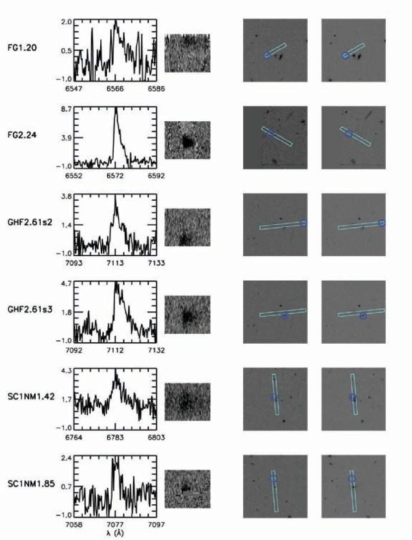
[p]

Figure 19.— Spectral ID, cutout of flux calibrated DEIMOS one-dimensional spectrum uncorrected for slit losses in units of $\mu$Jy, and cutout of DEIMOS two-dimensional spectrum for each LAE candidate. Postage stamps of the ACS F606W and F814W images (when available) or the LFC $r\arcmin$, $i\arcmin$, and $z\arcmin$ show the DEIMOS slit (box) and the LAE candidate position (circle) either from the detected position or inferred assuming the LAE fell in the middle of the slit (widthwise). LAE candidates 1 through 6.

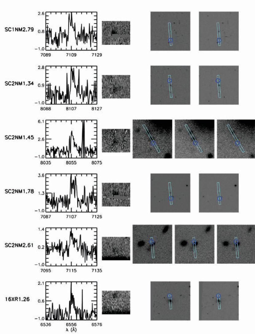
Figure 20.— LAE candidates 7 through 12.

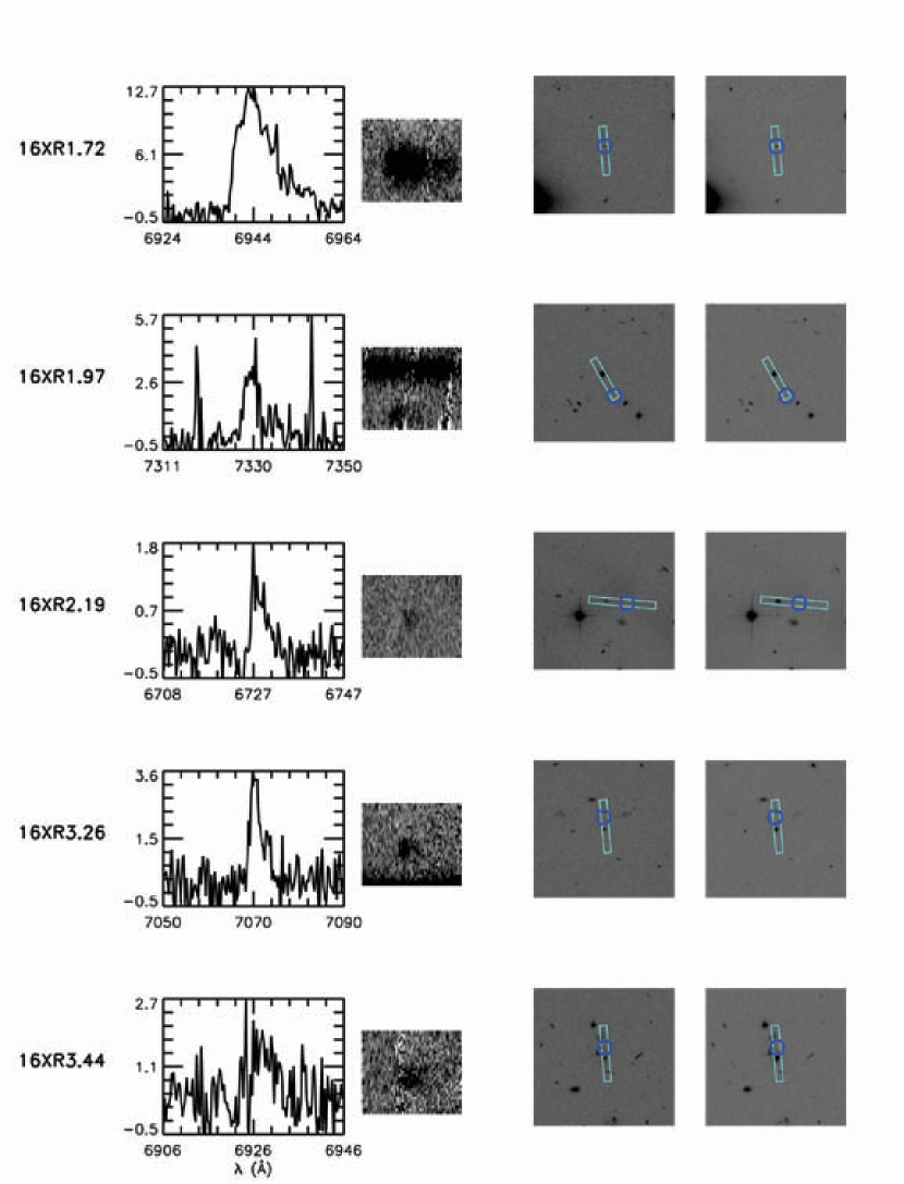
Figure 21.— LAE candidates 13 through 17.

Table 1Properties of LAE candidates not detected in the imaging

$ID$	$z$	$\alpha_{2000}$	$\delta_{2000}$b	Class	$F_{Ly\alpha}$	$L_{Ly\alpha}$d	SFR d,	$m_{F606W}$	$m_{F814W}$f	$r\arcmin^{f}$	$i\arcmin^{f}$	$z\arcmin^{f}$	$EW$ e,	$EW_{t}$ e,	$EW_{r}$ e,	$EW_{t,r}$ e,	$\lambda_{em}$
					($10^{-18}$ ergs s-1 $\rm{cm}^{-2}$)	($10^{42}$ erg s-1)	$\left(\rm{M}_{\odot}\rm{yr}^{-1}\right)$						(Å)	(Å)	(Å)	(Å)	(Å)
FG2.24	4.40632	241.106979	43.349430	2	$19.69_{-7.20}^{+11.26}$	$3.82_{-1.40}^{+2.18}$	$5.52_{-2.02}^{+3.16}$	25.24	24.79	25.63	25.34	24.03	$>$28.7	$>$143.4	$>$19.0	$>$137.0	6572.5
GHF2.61s2	4.85077	240.996353	43.413406	3	$10.37_{-3.83}^{+5.95}$	$2.52_{-0.93}^{+1.45}$	$4.01_{-1.48}^{+2.30}$	25.28	24.88	25.72	25.20	24.01	$>$13.6	$>$65.4	$>$11.9	$>$62.4	7112.8
SC1NM1.42	4.57989	241.111909	43.186732	2	$9.17_{-3.41}^{+5.28}$	$1.95_{-0.72}^{+1.12}$	$2.92_{-1.08}^{+1.69}$	25.36	24.83	25.00	25.13	23.39	$>$12.1	$>$55.1	$>$9.5	$>$52.6	6783.5
SC1NM1.85	4.82165	241.073486	43.310581	1	$4.92_{-1.91}^{+2.88}$	$1.18_{-0.45}^{+0.69}$	$1.87_{-0.72}^{+1.09}$	25.40	24.85	25.69	25.32	23.89	$>$6.7	$>$27.7	$>$4.8	$>$26.4	7077.4
SC1NM2.79	4.84754	241.066261	43.310909	1	$3.71_{-1.43}^{+2.17}$	$0.90_{-0.35}^{+0.53}$	$1.44_{-0.55}^{+0.84}$	24.98	24.58	25.72	25.31	23.98	$>$4.0	$>$18.8	$>$3.1	$>$18.0	7108.9
SC2NM1.34	5.66885	241.118866	43.204311	3	$4.63_{-1.80}^{+2.72}$	$1.62_{-0.63}^{+0.95}$	$2.93_{-1.14}^{+1.72}$	25.41	24.87	25.21	25.31	23.61	$>$4.5	$>$21.4	…	…k	8107.3
SC2NM1.45	5.62570	241.196610	43.212936	3	$5.56_{-2.14}^{+3.25}$	$1.91_{-0.74}^{+1.12}$	$3.45_{-1.33}^{+2.02}$	…	…l	26.18	25.22	23.67	$>$6.6	…	…k	…k	8054.9
SC2NM1.78	4.84561	241.140350	43.334343	1	$6.22_{-2.38}^{+3.63}$	$1.51_{-0.57}^{+0.88}$	$2.40_{-0.92}^{+1.40}$	26.11	25.62	25.59	25.17	23.93	$>$15.0	$>$78.5	$>$11.9	$>$86.0	7106.5
SC2NM2.61	4.85259	241.181778	43.274860	3	$2.94_{-1.19}^{+1.76}$	$0.72_{-0.29}^{+0.43}$	$1.14_{-0.46}^{+0.68}$	…l	…l	25.94	24.87	23.65	$>$4.6	…m	$>$2.1	…m	7115.0
16XR1.26	4.39288	241.089600	43.244692	3	$3.68_{-1.57}^{+2.26}$	$0.71_{-0.30}^{+0.44}$	$1.02_{-0.43}^{+0.62}$	25.25	24.70	25.60	25.28	23.94	$>$3.2	$>$16.3	$>$2.5	$>$15.5	6556.1
16XR1.97	5.02973	241.094269	43.292652	1	$8.97_{-3.38}^{+5.20}$	$2.37_{-0.90}^{+1.38}$	$3.92_{-1.48}^{+2.27}$	25.44	24.92	25.57	25.37	23.96	$>$11.5	$>$47.1	$>$8.5	$>$44.9	7330.3
16XR2.19	4.53375	240.858124	43.356789	3	$2.84_{-1.11}^{+1.67}$	$0.59_{-0.23}^{+0.35}$	$0.88_{-0.35}^{+0.52}$	25.43	24.94	25.43	24.91	23.86	$>$3.3	$>$13.7	$>$2.5	$>$12.9	6727.4
16XR3.26	4.81549	240.968445	43.382172	3	$6.75_{-2.57}^{+3.93}$	$1.61_{-0.61}^{+0.94}$	$2.56_{-0.97}^{+1.49}$	25.50	24.95	25.60	25.21	23.86	$>$6.0	$>$23.6	$>$4.5	$>$37.6	7069.9
16XR3.44	4.69732	240.017355	43.286700	2	$4.90_{-2.16}^{+3.05}$	$1.11_{-0.49}^{+0.69}$	$1.71_{-0.75}^{+1.06}$	25.47	24.88	25.68	25.27	23.94	$>$4.3	$>$17.0	$>$3.2	$>$16.2	6926.2

Table 2Properties of LAE candidates detected in the imaging

$ID$

$z$

$\alpha_{2000}$

$\delta_{2000}$

Class

$F_{Ly\alpha}$

$L_{Ly\alpha}$a

SFR a,

SFRUV

MUVc

$m_{F606W}$

$m_{F814W}$

$r\arcmin$

$i\arcmin$

$z\arcmin$

$EW$ b,

$EW_{r}$ b,

$\lambda_{em}$

($10^{-18}$ ergs s-1 $\rm{cm}^{-2}$)

($10^{42}$ erg s-1)

$\rm{M}_{\odot}$ yr-1

$\rm{M}_{\odot}$ yr-1

(Å)

(Å)

(Å)

FG1.20

4.40149

241.066400

43.343734

2

$8.84_{-3.36}^{+5.14}$

$1.71_{-0.65}^{+0.99}$

$2.47_{-0.94}^{+1.43}$

$14.0_{-1.30}^{+1.43}$

-21.02

25.53

25.16

25.31

24.41

…

$>$11.0

$>$12.1

6566.6

GHF2.61s3

4.85025

240.991890

43.413297

2

$16.07_{-5.88}^{+9.20}$

$3.92_{-1.44}^{+2.24}$

$6.24_{-2.28}^{+3.58}$

$9.91_{-0.93}^{+0.88}$

-20.65

26.89

25.70

…f

…f

…f

$>$37.3

$>$66.8

7112.1

16XR1.72

4.71230

241.062630

43.323880

3

$75.42_{-27.44}^{+43.06}$

$17.12_{-6.23}^{+9.78}$

$26.52_{-9.65}^{+15.14}$

$29.75_{-0.84}^{+0.79}$

-21.85

25.71

24.45

25.43

24.11

24.17

$>$60.6

$>$152.4

6944.4

References

- Ahn (2004) Ahn, S.-H. 2004, ApJ, 601, L25
- Ajiki et al. (2003) Ajiki, M., et al. 2003, AJ, 126, 2091
- Baldwin et al. (1981) Baldwin, J. A., Phillips, M. M., & Terlevich, R. 1981, PASP, 93, 5
- Becker et al. (2001) Becker, R. H., et al. 2001, AJ, 122, 2850
- Boughn et al. (1986) Boughn, S. P., Saulson, P. R., & Uson, J. M. 1986, ApJ, 301, 17
- Bouwens et al. (2003) Bouwens, R. J., et al. 2003, ApJ, 595, 589
- Bouwens et al. (2004a) Bouwens, R. J., et al. 2004, ApJ, 606, L25
- Bouwens et al. (2004b) Bouwens, R. J., et al. 2004, ApJ, 616, L79
- Bouwens et al. (2006) Bouwens, R. J., Illingworth, G. D., Blakeslee, J. P., & Franx, M. 2006, ApJ, 653, 53
- Brinchmann et al. (2004) Brinchmann, J., Charlot, S., White, S. D. M., Tremonti, C., Kauffmann, G., Heckman, T., & Brinkmann, J. 2004, MNRAS, 351, 1151
- Brocklehurst (1971) Brocklehurst, M. 1971, MNRAS, 153, 471
- Bunker et al. (2004) Bunker, A. J., Stanway, E. R., Ellis, R. S., & McMahon, R. G. 2004, MNRAS, 355, 374
- Cooper (2007) Cooper, M. C. 2007, Ph.D. Thesis
- Crampton & Lilly (1999) Crampton, D., & Lilly, S. 1999, Photometric Redshifts and the Detection of High Redshift Galaxies, 191, 229
- Davis & Wilkinson (1974) Davis, M., & Wilkinson, D. T. 1974, ApJ, 192, 251
- Davis et al. (2003) Davis, M., et al. 2003, Proc. SPIE, 4834, 161
- Davis (1980) Davis, M. 1980, Objects of High Redshift, 92, 57
- Dawson et al. (2002) Dawson, S., Spinrad, H., Stern, D., Dey, A., van Breugel, W., de Vries, W., & Reuland, M. 2002, ApJ, 570, 92
- Dawson et al. (2004) Dawson, S., et al. 2004, ApJ, 617, 707
- Dawson et al. (2007) Dawson, S., Rhoads, J. E., Malhotra, S., Stern, D., Wang, J., Dey, A., Spinrad, H., & Jannuzi, B. T. 2007, ApJ, 671, 1227
- de Propris et al. (1993) de Propris, R., Pritchet, C. J., Hartwick, F. D. A., & Hickson, P. 1993, AJ, 105, 1243
- Djorgovski et al. (2001) Djorgovski, S. G., Castro, S., Stern, D., & Mahabal, A. A. 2001, ApJ, 560, L5
- Egami et al. (2005) Egami, E., et al. 2005, ApJ, 618, L5
- Elston et al. (1989) Elston, R., Rieke, M. J., & Rieke, G. H. 1989, ApJ, 341, 80
- Faber et al. (2003) Faber, S. M., et al. 2003, Proc. SPIE, 4841, 1657
- Fan et al. (2006) Fan, X., et al. 2006, AJ, 132, 117
- Ferguson et al. (2004) Ferguson, H. C., et al. 2004, ApJ, 600, L107
- Franx et al. (1997) Franx, M., Illingworth, G. D., Kelson, D. D., van Dokkum, P. G., & Tran, K.-V. 1997, ApJ, 486, L75
- Fricke et al. (2001) Fricke, K. J., Izotov, Y. I., Papaderos, P., Guseva, N. G., & Thuan, T. X. 2001, AJ, 121, 169
- Fukugita et al. (1996) Fukugita, M., Ichikawa, T., Gunn, J. E., Doi, M., Shimasaku, K., & Schneider, D. P. 1996, AJ, 111, 1748
- Gal et al. (2008) Gal, R. R., Lemaux, B. C., Lubin, L. M., Kocevksi, D., & Squires, G. K. 2008, ApJ, 684, 933
- Giavalisco et al. (2004) Giavalisco, M., et al. 2004, ApJ, 600, L103
- Gronwall et al. (2007) Gronwall, C., et al. 2007, ApJ, 667, 79
- Guseva et al. (2003) Guseva, N. G., Papaderos, P., Izotov, Y. I., Green, R. F., Fricke, K. J., Thuan, T. X., & Noeske, K. G. 2003, A&A, 407, 75
- Hamana et al. (2008) Hamana, T., Miyazaki, S., Kashikawa, N., Ellis, R. S., Massey, R. J., Refregier, A., & Taylor, J. E. 2008, arXiv:0808.3813
- Hansen & Oh (2006) Hansen, M., & Oh, S. P. 2006, MNRAS, 367, 979
- Hinshaw et al. (2009) Hinshaw, G., et al. 2009, ApJS, 180, 225
- Hu et al. (2004) Hu, E. M., Cowie, L. L., Capak, P., McMahon, R. G., Hayashino, T., & Komiyama, Y. 2004, AJ, 127, 563
- Iwata et al. (2007) Iwata, I., Ohta, K., Tamura, N., Akiyama, M., Aoki, K., Ando, M., Kiuchi, G., & Sawicki, M. 2007, MNRAS, 376, 1557
- Izotov et al. (2006) Izotov, Y. I., Papaderos, P., Guseva, N. G., Fricke, K. J., & Thuan, T. X. 2006, A&A, 454, 137
- Kashikawa et al. (2006) Kashikawa, N., et al. 2006, ApJ, 637, 631
- Kehrig et al. (2004) Kehrig, C., Telles, E., & Cuisinier, F. 2004, AJ, 128, 1141
- Kennicutt (1998) Kennicutt, R. C., Jr. 1998, ARA&A, 36, 189
- Kirby et al. (2007) Kirby, E. N., Guhathakurta, P., Faber, S. M., Koo, D. C., Weiner, B. J., & Cooper, M. C. 2007, ApJ, 660, 62
- Kniazev et al. (2004) Kniazev, A. Y., Grebel, E. K., Pustilnik, S. A., Pramskij, A. G., Kniazeva, T. F., Prada, F., & Harbeck, D. 2004, AJ, 127, 704
- Koo & Kron (1980) Koo, D. C., & Kron, R. T. 1980, PASP, 92, 537
- Kurk et al. (2004) Kurk, J. D., Pentericci, L., Overzier, R. A., Röttgering, H. J. A., & Miley, G. K. 2004, A&A, 428, 817
- (48) agattuta, D. J., Lubin, L. M., Kocevski, D., Fassnacht, C. D., Gal, R. R, Lemaux, B. C., & Squires, G. K. 2010, in prep
- Lubin et al. (2009) Lubin, L. M., Gal, R. R., Lemaux, B. C., Kocevski, D. D., & Squires, G. K. 2009, AJ, 137, 4867
- Madau (1995) Madau, P. 1995, ApJ, 441, 18
- Madau et al. (1998) Madau, P., Pozzetti, L., & Dickinson, M. 1998, ApJ, 498, 106
- Malhotra & Rhoads (2002) Malhotra, S., & Rhoads, J. E. 2002, ApJ, 565, L71
- Malhotra & Rhoads (2004) Malhotra, S., & Rhoads, J. E. 2004, ApJ, 617, L5
- Mandelbaum et al. (2006) Mandelbaum, R., Seljak, U., Cool, R. J., Blanton, M., Hirata, C. M., & Brinkmann, J. 2006, MNRAS, 372, 758
- Margoniner et al. (2005) Margoniner, V. E., Lubin, L. M., Wittman, D. M., & Squires, G. K. 2005, AJ, 129, 20
- Martin & Sawicki (2004) Martin, C. L., & Sawicki, M. 2004, ApJ, 603, 414
- Martin et al. (2008) Martin, C. L., Sawicki, M., Dressler, A., & McCarthy, P. 2008, ApJ, 679, 942
- Mas-Hesse et al. (2003) Mas-Hesse, J. M., Kunth, D., Tenorio-Tagle, G., Leitherer, C., Terlevich, R. J., & Terlevich, E. 2003, ApJ, 598, 858
- Meiksin (2006) Meiksin, A. 2006, MNRAS, 365, 807
- Miley et al. (2004) Miley, G. K., et al. 2004, Nature, 427, 47
- Milvang-Jensen et al. (2008) Milvang-Jensen, B., et al. 2008, A&A, 482, 419
- Murayama et al. (2007) Murayama, T., et al. 2007, ApJS, 172, 523
- Navarro et al. (1996) Navarro, J. F., Frenk, C. S., & White, S. D. M. 1996, ApJ, 462, 563
- Oke & Gunn (1983) Oke, J. B., & Gunn, J. E. 1983, ApJ, 266, 713
- Osterbrock (1989) Osterbrock, D. E. 1989, Research supported by the University of California, John Simon Guggenheim Memorial Foundation, University of Minnesota, et al. Mill Valley, CA, University Science Books, 1989, 422 p.
- Ouchi et al. (2003) Ouchi, M., et al. 2003, ApJ, 582, 60
- Ouchi et al. (2008) Ouchi, M., et al. 2008, ApJS, 176, 301
- Overzier et al. (2006) Overzier, R. A., et al. 2006, ApJ, 637, 58
- Overzier et al. (2008) Overzier, R. A., e al. 2008, ApJ, 673, 143
- Partridge (1974) Partridge, R. B. 1974, ApJ, 192, 241
- Petrosian et al. (2002) Petrosian, A. R., Movsessian, T., Comte, G., Kunth, D., & Dodonov, S. 2002, A&A, 391, 487
- Poggianti et al. (2006) Poggianti, B. M., et al. 2006, ApJ, 642, 188
- Poggianti et al. (2008) Poggianti, B. M., et al. 2008, ApJ, 684, 888
- Pritchet & Hartwick (1987) Pritchet, C. J., & Hartwick, F. D. A. 1987, ApJ, 320, 464
- Pritchet & Hartwick (1990) Pritchet, C. J., & Hartwick, F. D. A. 1990, ApJ, 355, L11
- Reverte et al. (2007) Reverte, D., Vílchez, J. M., Hernández-Fernández, J. D., & Iglesias-Páramo, J. 2007, AJ, 133, 705
- Rhoads et al. (2000) Rhoads, J. E., Malhotra, S., Dey, A., Stern, D., Spinrad, H., & Jannuzi, B. T. 2000, ApJ, 545, L85
- Rhoads & Malhotra (2001) Rhoads, J. E., & Malhotra, S. 2001, ApJ, 563, L5
- Rhoads et al. (2003) Rhoads, J. E., et al. 2003, AJ, 125, 1006
- Richard et al. (2009) Richard, J., Pei, L., Limousin, M., Jullo, E., & Kneib, J. P. 2009, A&A, 498, 37
- Santos et al. (2004) Santos, M. R., Ellis, R. S., Kneib, J.-P., Richard, J., & Kuijken, K. 2004, ApJ, 606, 683
- Saulson & Boughn (1982) Saulson, P., & Boughn, S. 1982, BAAS, 14, 630
- Sawicki et al. (2008) Sawicki, M., et al. 2008, ApJ, 687, 884
- Sawicki & Thompson (2006) Sawicki, M., & Thompson, D. 2006, ApJ, 648, 299
- Schechter (1976) Schechter, P. 1976, ApJ, 203, 297
- Shapley et al. (2003) Shapley, A. E., Steidel, C. C., Pettini, M., & Adelberger, K. L. 2003, ApJ, 588, 65
- Shapley et al. (2005) Shapley, A. E., Coil, A. L., Ma, C.-P., & Bundy, K. 2005, ApJ, 635, 1006
- Shimasaku et al. (2003) Shimasaku, K., et al. 2003, ApJ, 586, L111
- Shimasaku et al. (2005) Shimasaku, K., Ouchi, M., Furusawa, H., Yoshida, M., Kashikawa, N., & Okamura, S. 2005, PASJ, 57, 447
- Shimasaku et al. (2006) Shimasaku, K., et al. 2006, PASJ, 58, 313
- Simcoe et al. (2000) Simcoe, R. A., Metzger, M. R., Small, T. A., & Araya, G. 2000, Bulletin of the American Astronomical Society, 32, 758
- Spergel et al. (2007) Spergel, D. N., et al. 2007, ApJS, 170, 377
- Stanway et al. (2004) Stanway, E. R., et al. 2004, ApJ, 604, L13
- Stanway et al. (2007) Stanway, E. R., et al. 2007, MNRAS, 376, 727
- Stark et al. (2007) Stark, D. P., Ellis, R. S., Richard, J., Kneib, J.-P., Smith, G. P., & Santos, M. R. 2007, ApJ, 663, 10
- Steidel et al. (1996a) Steidel, C. C., Giavalisco, M., Pettini, M., Dickinson, M., & Adelberger, K. L. 1996, ApJ, 462, L17
- Steidel et al. (1996b) Steidel, C. C., Giavalisco, M., Dickinson, M., & Adelberger, K. L. 1996, AJ, 112, 352
- Steidel et al. (2000) Steidel, C. C., Adelberger, K. L., Shapley, A. E., Pettini, M., Dickinson, M., & Giavalisco, M. 2000, ApJ, 532, 170
- Stern et al. (2005) Stern, D., Yost, S. A., Eckart, M. E., Harrison, F. A., Helfand, D. J., Djorgovski, S. G., Malhotra, S., & Rhoads, J. E. 2005, ApJ, 619, 12
- Taniguchi et al. (2005) Taniguchi, Y., et al. 2005, PASJ, 57, 165
- Thompson & Djorgovski (1995) Thompson, D., & Djorgovski, S. G. 1995, AJ, 110, 982
- Thompson et al. (1995) Thompson, D., Djorgovski, S., & Trauger, J. 1995, AJ, 110, 963
- Tran et al. (2004) Tran, K.-V. H., Lilly, S. J., Crampton, D., & Brodwin, M. 2004, ApJ, 612, L89
- Venemans et al. (2004) Venemans, B. P., et al. 2004, A&A, 424, L17
- Venemans et al. (2005) Venemans, B. P., et al. 2005, A&A, 431, 793
- Westra et al. (2005) Westra, E., et al. 2005, A&A, 430, L21
- Westra et al. (2006) Westra, E., et al. 2006, A&A, 455, 61
- Yan et al. (2006) Yan, R., Newman, J. A., Faber, S. M., Konidaris, N., Koo, D., & Davis, M. 2006, ApJ, 648, 281
- Yoshida et al. (2006) Yoshida, M., et al. 2006, ApJ, 653, 988
- Zheng et al. (2006) Zheng, W., et al. 2006, ApJ, 640, 574