Towards Chip-on-Chip Neuroscience:
Fast Mining of Frequent Episodes Using Graphics Processors

Abstract

Computational neuroscience is being revolutionized with the advent of multi-electrode arrays that provide real-time, dynamic, perspectives into brain function. Mining event streams from these chips is critical to understanding the firing patterns of neurons and to gaining insight into the underlying cellular activity. We present a GPGPU solution to mining spike trains. We focus on mining frequent episodes which captures coordinated events across time even in the presence of intervening background/“junk” events. Our algorithmic contributions are two-fold: MapConcatenate, a new computation-to-core mapping scheme, and a two-pass elimination approach to quickly find supported episodes from a large number of candidates. Together, they help realize a real-time “chip-on-chip” solution to neuroscience data mining, where one chip (the multi-electrode array) supplies the spike train data and another (the GPGPU) mines it at a scale unachievable previously. Evaluation on both synthetic and real datasets demonstrate the potential of our approach.

Keywords: Frequent episode mining, GPGPU, spike train datasets, computational neuroscience.

1 Introduction

Temporal (symbolic) event streams are popular in scientific domains, such as physical plants, medical diagnostics, and neuroscience. In all these domains, we are given occurrences of events of interest over a time course and the goal is to identify trends and behaviors that serve discriminatory or descriptive purposes. In this paper, we focus exclusively on event streams gathered through multi-electrode array (MEA) chips for studying neuronal function although our algorithms and implementations are applicable to a wider variety of domains.

An MEA records spiking action potentials from an ensemble of neurons which after various pre-processing steps, yields a spike train dataset providing real-time, dynamic, perspectives into brain function (see Figure 1). Identifying sequences (e.g., cascades) of firing neurons, determining their characteristic delays, and reconstructing the functional connectivity of neuronal circuits are key problems of interest. This provides critical insights into the cellular activity recorded in the neuronal tissue.

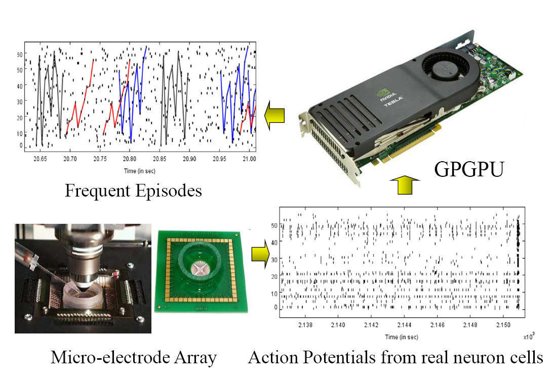
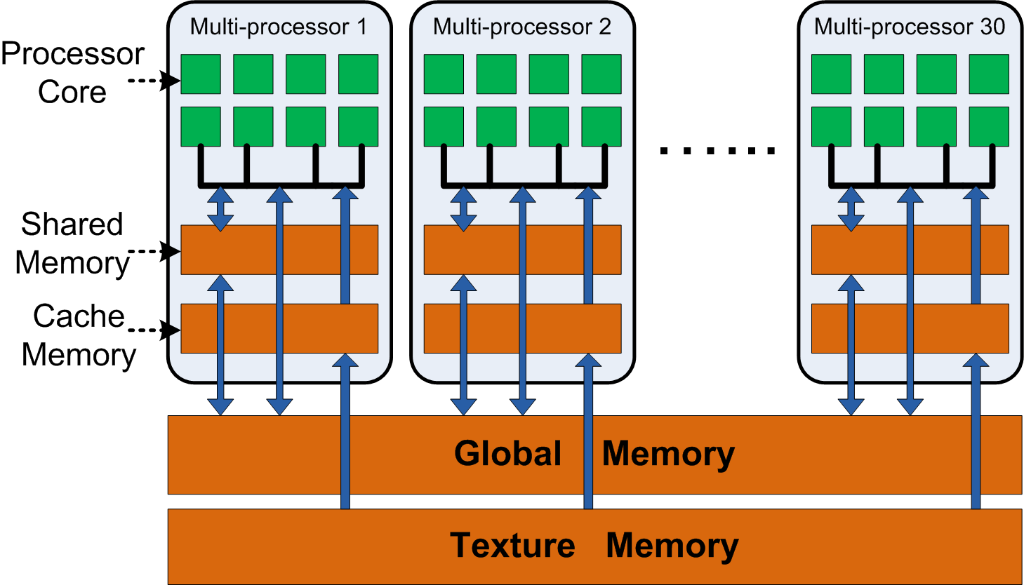
Figure 1: (left) Chip-on-Chip neuroscience: spike trains recorded from a multi-electrode array (MEA) are mined by a GPGPU to yield frequent episodes which can be summarized to reconstruct the underlying neuronal circuitry. (right) Architecture of the NVIDIA GTX280 GPGPU in detail.

With rapid developments in instrumentation and data acquisition technology, the size of event streams recorded by MEAs has concomitantly grown, leading us to exhaust the abilities of sequential computation. For instance, just a few minutes of cortical recording from a 64-channel MEA can easily generate millions of spikes! It has thus become imperative to enable fast, near real-time computation, data mining, and visualization of mined patterns. This mapping is critical as it can result in orders-of-magnitude difference in performance.

We adopt GPGPUs as the platform of choice for neuroscience data mining for several reasons. First, they are particularly economical in morphing a desktop into a rather powerful parallel computing machine (price-to-performance ratio). This is especially attractive to neuroscientists who might not have access to clusters of workstations. At the same time, mapping our application to a GPGPU architecture is non-trivial. GPGPUs were originally designed for data-parallel applications (e.g., rendering), not quite the class of problems that temporal data mining falls under. Our main contributions are as follows:

1. MapConcatenate, a computation-to-core mapping scheme suitable for frequent episode mining that takes advantage of the computational power of hundreds of processing cores on a GPU. MapConcatenate is a two-stage scheme like MapReduce [Dean:2004] but quite different in the intent and applicability of both the stages.

2. A two-pass elimination approach to find supported temporal episodes from a large number of candidates. The first pass, which is conducted with relaxed timing constraints, can eliminate most of the non-supported episode candidates with the accurate count computed using the second pass. Design of this elimination approach and proving its correctness is non-trivial since the set of episodes returned by the relaxed set of constraints is not a superset of the original set of constraints but the counts are indeed an upper bound.

3. A ‘chip-on-chip’ real-time solution to neuroscience data mining where one chip (the MEA) provides the data and another chip (the graphics processor) mines it. Our solution is not a complete data streaming solution; nevertheless, we achieve real-time responsiveness by processing partitions of the data stream in turn.

2 Problem Statement

A spike train dataset can be modeled as an event stream, where each symbol/event type corresponds to a specific neuron (or clump of neurons) and the dataset encodes occurrence times of these events over the time course.

Definition 2.1.

An event stream is denoted by a sequence of events $\langle(E_{1},t_{1}),(E_{2},t_{2}),\ldots(E_{n},t_{n})\rangle$, where $n$ is the total number of events. Each event $(E_{i},t_{i})$ is characterized by an event type $E_{i}$ and a time of occurrence $t_{i}$. The sequence is ordered by time i.e. $t_{i}\leq t_{i+1}\forall i=1,\ldots,n-1$ and $E_{i}$’s are drawn from a finite set $\xi$.

One class of interesting patterns that we wish to discover are frequently occurring groups of events (i.e., firing cascades of neurons) with some constraints on ordering and timing of these events. This is captured by the notion of episodes, the original framework for which was proposed by Mannila et al [window].

Definition 2.2.

An (serial) episode $\alpha$ is an ordered tuple of event types $V_{\alpha}\subseteq\xi$.

For example $(A\rightarrow B\rightarrow C\rightarrow D)$ is a 4-node serial episode, and it captures the pattern that neuron A fires, followed by neurons B, C and D in that order, but not necessarily without intervening ‘junk’ firings of neurons (even possibly neurons A, B, C, or D). This ability to intersperse noise or don’t care states, of arbitrary length, between the event symbols in the definition of an episode is what makes these patterns non-trivial, useful, and comprehensible.

Frequency of episodes: The notion of frequency of an episode can be defined in several ways. In [window], it is defined as the fraction of windows in which the episode occurs. Another measure of frequency is the non-overlapped count which is the size of the largest set of non-overlapped occurrences of an episode. Two occurrences are non-overlapped if no event of one occurrence appears in between the events of the other. In the event stream of Fig. 2, there are at most two non-overlapped occurrences of the episode $A\rightarrow B$, although there are 8 occurrences in total.

We use the non-overlapped occurrence count as the frequency measure of choice due to its strong theoretical properties under a generative model of events [vatsan2]. It has also been argued in [Patnaik2008] that, for the neuroscience application, counting non-overlapped occurrences is natural because episodes then correspond to causative, “syn-fire”, chains that happen at different times again and again.

Temporal constraints: Besides the frequency threshold, a further level of constraint can be imposed on the definition of episodes. In multi-neuronal datasets, if one would like to infer that neuron $A$’s firings cause a neuron $B$ to fire, then spikes from neuron $B$ cannot occur immediately or spontaneously after $A$’s spikes due to axonal conduction delays. These spikes cannot also occur too much later than $A$ for the same reason. Such minimum and maximum inter-event delays are common in other application domains as well. We hence place inter-event time constraints giving rise to episodes such as:

$$(A^{\underrightarrow{(t_{low}^{1},t_{high}^{1}]}}B^{\underrightarrow{(t_{low}^{2},t_{high}^{2}]}}C)$$

In a given occurrence of episode $A\rightarrow$ $B\rightarrow$ $C$ let $t_{A}$, $t_{B}$, and $t_{C}$ denote the time of occurrence of corresponding event types. A valid occurrence of the serial episode satisfies

$$t_{low}^{1}<(t_{B}-t_{A})\leq t_{high}^{1},t_{low}^{2}<(t_{C}-t_{B})\leq t_{high}^{2}$$

(In general, an $N$-node serial episode is associated with $N-1$ inter-event constraints.) In Fig. 2, there is exactly one occurrence of the episode $A\stackrel{{\scriptstyle(5,10]}}{{\rightarrow}}B\stackrel{{\scriptstyle(10,15]}}{{\rightarrow}}C$ satisfying the desired inter-event constraints (shown in dotted boxes).

Problem 1: Given an event stream $\{(E_{i},t_{i})\}$, $i\in\{1\ldots{n}\}$, a set of inter-event constraints $I=\{(t_{low}^{k},t_{high}^{k}]\}$,$k\in\{1\ldots{l}\}$,  find all serial episodes $\alpha$ of the form:

$$\alpha=\langle E_{(1)}^{\underrightarrow{(t_{low}^{(1)},t_{high}^{(1)}]}}E_{(2)}\ldots^{\underrightarrow{(t_{low}^{(N-1)},t_{high}^{(N-1)}]}}E_{(N)}\rangle$$

such that the non-overlapped occurrence counts of each episode $\alpha$ is $\geq\theta$, a user-specified threshold. Here $E_{(.)}$’s are the event types in the episode $\alpha$ and $(t_{low}^{(.)},t_{high}^{(.)}]$’s $\in I$ are the corresponding inter-event constraints.

3 Prior Work

We review prior work in three categories: mining frequent episodes, data mining using GPGPUs, and the map-reduce framework for large scale computations.

Mining Frequent Episodes: The overall mining procedure for frequent episodes is based on level-wise mining. Within this framework there are two broad classes of algorithms: window-based [window] and state machine based [fsa-mining, vatsan2], and they primarily differ in how they define the frequency of an episode. The window based algorithms define frequency of an episode as the fraction of windows on the event sequence in which the episode occurs. The state machine based algorithms are more efficient and define frequency as the size of largest set of non-overlapped occurrences of an episode. Within the class of state machine algorithms, serial episode discovery using non-overlapped counts was described in [vatsan2], and their extension to temporal constraints is given in [Patnaik2008]. With the introduction of temporal constraints the state machine based algorithms become more complicated. They must keep track of what part of an episode has been seen, which event is expected next and, when episodes inter-leave, they must make a decision of which events to be used in the formation of an episode.

Data Mining Using GPGPUs: Many researchers have harnessed the capabilities of GPGPUs for data mining. The key to porting a data mining algorithm onto a GPGPU is to, in one sense, “dumb it down”; i.e., conditionals, program branches, and complex decision constraints are not easily parallelizable on a GPGPU and algorithms using these constraints will require significant reworking to fit this architecture (temporal episode mining unfortunately falls in this category). There are many emerging publications in this area but due to space restrictions, we survey only a few here. The SIGKDD tutorial by Guha et al. [tutorial] provides a gentle introduction to the aspects of data mining on GPGPUs through problems like k-means clustering, reverse nearest neighbor(RNN), discrete wavelet transform(DWT), sorting networks, etc. In [dmg2], a bitmap technique is proposed to support counting and is used to design GPGPU variants of Apriori and k-means clustering. This work also proposes co-processing for itemset mining where the complicated tie data structure is kept and updated in the main memory of CPU and only the itemset counting is executed in parallel on GPU. A sorting algorithm on GPGPUs with applications to frequency counting and histogram construction is discussed in [dmg1] which essentially recreates sorting networks on the GPU. Li et al. [li-cut] present a ‘cut-and-stitch’ algorithm for approximate learning of Kalman filters. Although this is not a GPGPU solution per se, we point out that our proposed approach shares with this work the difficulties of mining temporal behavior in a parallel context.

MapReduce: Modeled after LISP primitives, MapReduce [Dean:2004] provides a distribution framework for large scale computations using two functions: map, and reduce. It has received a fair share of attention (and, sometimes, criticism) from the cloud computing and data-intensive computing communities. The framework has been ported to many platforms, including GPGPUs (e.g., see [mars]). See Section LABEL:sec:MapConcat for comparisons between our proposed framework and MapReduce.

4 GPGPU Architecture

To understand the algorithmic details behind our approach, we provide a brief overview of GPGPU and its architecture.

The initial purpose of specialized GPUs was to accelerate the display of 2D and 3D graphics, much in the same way that the FPU focused on accelerating floating-point instructions. However, the rapid technological advances of the GPU, coupled with extraordinary speed-ups of application “toy” benchmarks on the specialized GPUs, led GPU vendors to transform the GPU from a specialized processor to a general-purpose graphics processing unit (GPGPU), such as the NVIDIA GTX 280, as shown in Figure 1 (right). To lessen the steep learning curve, GPU vendors also introduced programming environments, such as the Compute Unified Device Architecture (CUDA).

Processing Elements: The basic execution unit on the GTX 280 is a scalar processing core, of which 8 together form a multiprocessor. While the number of multiprocessors and processor clock frequency depends on the make and model of the GPU, every multiprocessor in CUDA executes in SIMT (Single Instruction, Multiple Thread) fashion, which is similar in nature to SIMD (Single Instruction, Multiple Data) execution. Specifically, groups of 32 threads form a warp and execute the exact same codepath until every thread terminates. However, when codepaths diverge, each thread must now execute every instruction on every thread path, therefore, implying that optimal performance is attained when all 32 threads do not branch down different codepaths. The execution of a single instruction with 8 cores and a warp size of 32 completes in 4 cycles.

Memory Hierarchy: The GTX 280 contains multiple forms of memory. Beginning with the furthest from the GPU processing elements, the device memory is located off-chip on the graphics card and provides the main source of storage for the GPU while simultaneously being accessible from the CPU and GPU. Each multiprocessor on the GPU contains three caches — a texture cache, constant cache, and shared memory. The texture cache and constant cache are both read-only memory providing fast access to immutable data. Shared memory, on the other hand, is read-write to provide each core with fast access to the shared address space of a thread block within a multiprocessor. Finally, on each core resides a plethora of registers such that there exists minimal reliance on local memory resident off-chip on the device memory.

Parallelism Abstractions: At the highest level, the CUDA programming model requires the programmer to offload functionality to the GPGPU as a compute kernel. This kernel is evaluated as a set of thread blocks logically arranged in a grid to facilitate organization. In turn, each block contains a set of threads, which will be executed on the same multiprocessor, with the threads scheduled in warps, as mentioned above.

5 Algorithms

Our overall approach for solving Problem 1 is based on a state machine algorithm with inter-event constraints [Patnaik2008]. There are two major phases of this algorithm: generating episode candidates and counting these episodes, and we focus on the latter since it is the key performance bottleneck, typically by a few orders of magnitude. Therefore, we present a GPU-accelerated algorithm for counting episodes of various size, while candidate generation is executed sequentially on a CPU.

In this section, we first present the standard sequential algorithm for mining frequent episodes with inter-event constraints. Next, we introduce our GPU based algorithm (called $A1$). We then propose a two-pass counting approach, where the first counting pass eliminates most of unsupported episodes and the second counting pass completes the counting tasks for the remaining episodes. Since the first counting pass uses a less complex algorithm (called $A2$), the execution time saved at this step contributes to an overall performance gain even we go through two-pass counting ($A2+A1$).

5.1 Episode Mining with Inter-Event Constraints

Algorithm LABEL:alg:A1 outlines the serial counting procedure for a single episode $\alpha$. Briefly, it maintains a data structure $s$ which is a list of lists. Each list $s[k]$ in $s$ corresponds to an event type $E_{(k)}\in\alpha$ and stores the times of occurrences of those events with event-type $E_{(k)}$ which satisfy the inter-event constraint $(t_{low}^{(k-1)},t_{high}^{(k-1)}]$ with at least one entry $t_{j}\in s[k-1]$. This requirement is relaxed for $s[0]$, thus every time an event $E_{(0)}$ is seen in the data its occurrence time is pushed into $s[0]$.

When an event of type $E_{(k)},2\leq{k}\leq{N}$ at time $t$ is seen, we look for an entry $t_{j}\in s[k-1]$ such that $t-t_{j}\in(t_{low}^{(k-1)},t_{high}^{(k-1)}]$. Therefore, if we are able to add the event to the list $s[k]$, it implies that there exists at least one previous event with event-type $E_{(k-1)}$ in the data stream for the current event which satisfies the inter-event constraint between $E_{(k-1)}$ and $E_{(k)}$. Applying this argument recursively, if we are able to add an event with event-type $E_{(|\alpha|)}$ to its corresponding list in $s$, then there exists a sequence of events corresponding to each event type in $\alpha$ satisfying the respective inter-event constraints. Such an event marks the end of an occurrence after which the $count$ for $\alpha$ is incremented and the data structure $s$ is reinitialized. Figure 2 illustrates the data structure $s$ for counting $A\stackrel{{\scriptstyle(5,10]}}{{\rightarrow}}B\stackrel{{\scriptstyle(10,15]}}{{\rightarrow}}C$.

The maximality of the left-most and inner-most occurrence counts for a general serial episode has been shown in [vatsan2]. Similar arguments hold for the case of serial episodes with inter-event constraints and not shown here for lack of space.

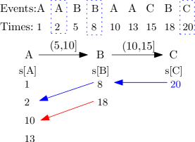
Figure 2: Illustration of the data structure $s$ for counting $A\stackrel{{\scriptstyle(5,10]}}{{\rightarrow}}B\stackrel{{\scriptstyle(10,15]}}{{\rightarrow}}C$