Epidemics with general generation interval distributions
Abstract
We study the spread of susceptible-infected-recovered (SIR) infectious diseases where an individual’s infectiousness and probability of recovery depend on his/her “age” of infection. We focus first on early outbreak stages when stochastic effects dominate and show that epidemics tend to happen faster than deterministic calculations predict. If an outbreak is sufficiently large, stochastic effects are negligible and we modify the standard ordinary differential equation (ODE) model to accommodate age-of-infection effects. We avoid the use of partial differential equations which typically appear in related models. We introduce a “memoryless” ODE system which approximates the true solutions. Finally, we analyze the transition from the stochastic to the deterministic phase.
1 Introduction
Infectious diseases continue to impact public health. The previous emergence of SARS, the ongoing emergence of H1N1 swine influenza, and the simmering threat of H5N1 avian influenza or other diseases call attention to the need to prepare for a quickly-spreading pandemic. Such a pandemic could have typical infectious period measured in days or weeks, spread worldwide, and grow quickly. In the face of such an emerging disease, there is little time to develop and implement interventions.
The ability to predict the timing and maximum patient load imposed by an epidemic is essential to intervention design. Overestimating the preparation time available or underestimating the peak may result in well-designed measures which are implemented too late or are too small.
The ability of an infectious disease to spread depends strongly on the number of susceptible individuals , and the total population size . We will find that the details of the spread are more sensative to changes in than changes in , and so we will couch most of our discussion in terms of changes in .
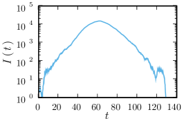
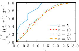
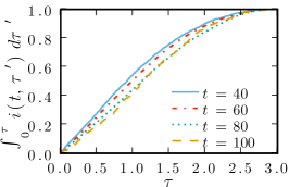
Figure 1 shows the course of an epidemic of an infectious disease whose characteristics are discussed later (§3.2.2 with ). At very early times the disease spreads as a branching process and stochastic effects are important. As the outbreak grows, the spread continues as a branching process, but the stochastic effects lose importance. However, the timing of the epidemic always feels the initial stochastic impact.
We also consider the infection-age distribution , the number of people infected at time who have been infected for units of time. We plot the cumulative distribution in figure 1 at small (center) and larger (right). At small the distributions are noisy, and converge to a steady-state distribution as increases. As the spread continues, begins to change perceptibly and the steady-state adjusts adiabatically if changes slowly enough. If does not change slowly, the system cannot adjust to the changing equilibrium. During the growing phase of the epidemic, the infected individuals are weighted towards more recent infections, while during the declining phase the infected individuals have disproportionately older infections.
We focus on several stages in this paper: the early stochastic phase, the later deterministic phase, and the transition phase between these two. If is initially small, then can change significantly during the stochastic phase. We do not address this case.
Typically disease outbreaks are either subcritical (meaning ) for which epidemics are impossible because an average infected person infects fewer than one individual, or supercritical (meaning ) for which epidemics are possible. We consider only supercritical outbreaks. Early in an outbreak’s spread, growth is dominated by stochastic effects, and it may die out stochastically. If it persists, it may grow faster or slower than “average”. As long as does not change significantly, the spread can be modeled using Crump-Mode-Jagers (CMJ) processes [7, 6, 12, 10]. A subcritical CMJ process dies out, while a supercritical CMJ process either dies out or converges to where is a random value and depends on the process.
If a supercritical outbreak becomes sufficiently large the spread is effectively deterministic. The usual equations for this phase are the susceptible-infected-recovered (SIR) equations
| (1) | ||||
| (2) | ||||
| (3) |
These equations assume that infected people cause infections at rate and recover at rate , giving an exponentially distributed infection duration. The process is “memoryless”. In contrast, for real diseases the “age” of an individual’s infection affects his/her infectiousness and probability of recovering.
Ignoring “age-of-infection” effects loses important details. During the growth of an epidemic the infections are biased towards young infection ages. If young infections are more (or less) infectious, the SIR equations under- (or over-) estimate the growth rate. Similar observations hold during decay.
Several approaches have been developed to study age-of-infection models. Some explicitly track the history of the epidemic [4, 11, 3, 2, 14, 5, 20]. Others attempt to maintain the memoryless feature of equations (1)–(3) by introducing a chain of infected compartments in order to approximate the infectious period distribution [1, 22, 17, 9, 15, 16]. These chains of compartments usually do not have biological meaning, but instead are a simplifying “trick”. Typically these assume constant and that each of infected classes recovers at rate , resulting in gamma-distributed infectious periods.
In this paper we investigate the growth of an epidemic from a single infection to a full-scale epidemic, without the restrictive assumptions underlying (1)–(3). In §2, we show how to model the early stochastic phase, and give some comparison with deterministic predictions. In §3 we show how to find deterministic equations governing the epidemic’s growth. We take a different approach from most previous studies and arrive at a system similar to the standard equations (1)–(3) rather than a partial differential equation. If the change in is not large during a typical infectious period, we can approximate the infectious population as being in equilibrium given and arrive at a memoryless system that captures the dynamics well. In §4 we examine what it means for the outbreak to be large enough to be deterministic.
2 Stochastic Phase
We assume that the disease spreads from individual to individual in such a way that the ability of individual to infect a susceptible individual depends only on how long has been infected and whether or not has recovered. We let be the probability is still infected units of time after becoming infected. If is still infected, the rate causes new infections is . This enforces a possibly unrealistic assumption that infectiousness is independent of infection duration. It would be straightforward to modify the model to incorporate this effect, but we do not do it here.
We have and — assuming no-one remains infectious forever — . We assume is differentiable. The probability of recovering in a short interval is . We let be the rate at which recovery happens: .
2.1 The equations
We have full derivations of the equations in appendix A. If is the probability that individuals are infected at time , then the probability generating function (pgf) provides a useful tool to help calculate . We get
| (4) |
Here is the pgf for the number of descendants an individual has units of time after its infection given that it recovers units of time after infection. That is is the probability an individual has infectious descendants units of time after becoming infected given that it recovers after units of time.
We find (for )
| (5) |
To find equations for we take the -th derivative of , divide by , and evaluate at . We solve the equations as described in appendix B.
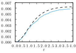
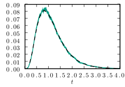
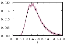
We compare the solutions with simulations in figure 2. We take the probability distribution function (pdf) of the infection duration to be a Weibull distribution, , so . We take constant . Although there is considerable noise in simulations, we find close match with analytic results.
2.2 Asymptotic behavior at large
If is large, then may still be approximately constant even as becomes much larger than . We are interested in the behavior of as it becomes large, but before has changed significantly. If we assume remains fixed, then under weak assumptions it can be shown [7, 6] that either becomes zero at some finite time or it converges to where is a random number determined by stochastic effects and solves
This equation is the Euler-Lotka (EL) equation, which we derive in §3. The solution is unique and known as the Malthusian parameter. The most significant assumption we require for this convergence is that the infection is not a “lattice” process, that is, possible times of infection are not discretized and so can change change continuously 111For lattice processes, similar results apply with discrete rather than continuous time.. This result guarantees that if the susceptible population is sufficiently large, the outbreak either dies out or becomes large enough that the growth is deterministic.
We have shown that equations (4) and (5) accurately predict the probability of having a given number of infections as a function of time. Once the outbreak is sufficiently large, the impact of stochastic effects is reduced and the infected population size scales like for fixed . The random value of determines how much time is available to prepare for the epidemic.
2.3 Distribution of epidemic onset times
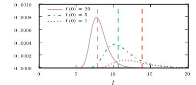
We turn to a simpler disease process to investigate the impact of the stochastic phase on how quickly an epidemic “takes off”. We consider a population with constant infectiousness and exponentially distributed infection durations (corresponding to a constant recovery rate). We compare predictions from the stochastic model with predictions from the deterministic equations (1)–(3) which are exactly valid precisely for this infection process. We take and .
Figure 3 shows that if the initial number of infections is low, it is relatively likely that the number infected becomes large before the deterministic equations predict it should. This has a number of implications for interpreting early stages of an outbreak. If we attempt to predict the present size of an outbreak given a known introduction date using the assumption of deterministic growth, we are likely to underpredict the current size. Consequently if we make preparations to introduce interventions under the assumption of deterministic growth, we may be using interventions that are too small and implemented too late.
The mismatch decreases as the initial number of infections increase. We explain this observation by noting that outbreaks with only a few infections grow on average at the deterministically predicted rate. However, those at the lower range of growth often go extinct, while those at the higher range tend to become epidemics quickly. This leads to the important conclusion that if an epidemic happens, it is likely to happen faster than the deterministic equations predict.
3 Deterministic Phase
In this section we develop the deterministic equations governing epidemics once stochastic effects are unimportant. Our exact equations are equivalent to many previous age-of-infection models [4, 11, 3, 2, 14, 5, 20], but we avoid the use of PDEs which usually arise. A related approach also avoiding PDEs was used by [3], but we cast our equations in a form similar to the standard SIR equations (1)–(3). We then introduce an approximation to these equations. We discuss the transition from the stochastic phase to the deterministic phase in §4.
In the stochastic phase analysis, we assumed that infectiousness is independent of the recovery time (except that after recovery infectiousness is zero). We can drop this assumption here and redefine as the average rate of infection units of time after infection for those individuals still infected (of which a fraction are successful). The product represents the expected rate of new infections caused by an individual infected units of time previously, where the expectation is taken without prior knowledge of whether has recovered. We normalize this by to arrive at the generation interval distribution [19, 21].
Let denote the rate of new infections occurring at time and the rate of recoveries. Let denote the number of people who became infected at time and are still infected at time . Then . We can find in terms of by and in terms of by .
If is constant the age-of-infection distribution converges to a steady-state where is independent of . The population size grows or decays exponentially, so where solves the modified EL equation
This has been used at early times [21] when to relate the exponential growth in time with .
We use the constant solution as the basis for our approach with changing . We take
Rearrangement gives
We derive equations for and in terms of as follows: The derivative of is . We multiply by , using to get
where . Repeating this for we get
where . This can be written in a similar form to the standard SIR equations, except that the coefficients change in time and depend on the history of the epidemic
| (6) | ||||
| (7) | ||||
| (8) | ||||
| (9) |
where and . Because of the similarity in notation, we distinguish to be the average rate of causing infection of all individuals infected at time , while is the average rate of causing infection by an individual still infected units of time after becoming infected. To initialize the problem we need for all as well as and . Typically we will assume that for so that . As we solve forward, new values of are calculated based on the change in . The history of for encodes all information needed about the age-of-infection distribution at . A less intuitive, but simpler formulation of these equations appears in appendix C.
3.1 Approximating the solution
Storing the history of an outbreak introduces some mild analytical and computational difficulties. It is convenient to work with a system that depends only on its current state. If varies slowly relative to how quickly changes, we can assume that the system responds adiabatically to changes in and so the age-of-infection distribution is at equilibrium with the current value of . This assumption will allow us to create equations analagous to (1)–(3) with changing coefficients, which may be solved by standard ODE methods. This approach will break down if changes significantly during a typical infectious period. Fortunately, we can use the results of the approximation to identify when the approximation fails.
We replace by where and approximate , , and by , , and respectively assuming that for the range of which make a significant contribution to the integral.
Note that each of these is a Laplace transform. The resulting approximating equations are
| (10) | ||||
| (11) | ||||
| (12) | ||||
| (13) |
where and .
Computationally this system of equations is only mildly more difficult than the standard SIR equations. We can either find the functional forms of the Laplace transforms, or simply calculate them for various in advance. Once that is done, then at each time step, we need only look at , identify such that , and then find and . Then the integration proceeds as in the standard SIR equations.
The approximation is valid as long as the amount of change of during a typical infectious period is small, and is therefore valid well into the nonlinear regime after the exponential growth phase has ended.
3.2 Examples
3.2.1 The usual suspects
If we make the usual assumptions of constant infectiousness and exponentially distributed recovery time [ constant and ] the system is memoryless. The function encodes the age-of-infection distribution, which is irrelevant in a memoryless system. Thus the equations for and should not depend on . We find , and so . We similarly find and so . So in this special case the exact age-of-infection model (6)–(9) reduces to the standard SIR equations (1)–(3). This holds even for our approximate system (10)–(13).
3.2.2 A piecewise continuous example
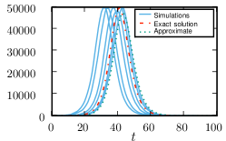
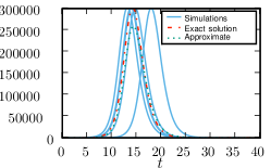
We take
| (14) | ||||
| (15) |
So people are initially infectious, then stop being infectious at and begin to recover. At , they continue recovering, but become infectious once more. By all individuals have recovered. Such a system could model a disease in which individuals are infectious before and possibly after having symptoms, but self-isolate during the symptomatic phase. The generation interval distribution is given by
| (16) |
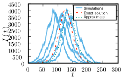
In figure 4 we find that the exact model (6)–(9) fits the simulations well (with the discrepancy due to stochastic shifts in time). The difference in timing between the exact and approximate solution (10)–(13) is due to differences in initial conditions: the exact calculation assumes a single infection beginning at while the approximate solution assumes that the epidemic begins with the equilibrium age-distribution already reached by . The approximate model is a good fit for the behavior at early times and remains a good approximation until the change in becomes significant over the duration of an infection. The approximation performs best in those situations where the number of infections remains smaller.
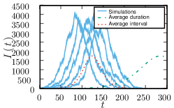
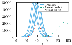
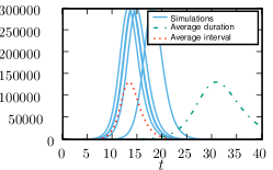
If we attempt to approximate the epidemic course using the standard SIR model (1)–(3), then we have two free parameters and . We can identify (at least) three constraints: , average duration of infection, and average generation interval. We can only match two of these at a time, which we show in figure 5. If we choose to match and average duration of infection then the total number of infected person-days is correct, but the timing is far off. If we choose to match and average generation interval, then the timing is much closer, but the peak patient load is significantly underestimated.
3.2.3 Gamma-distributed recovery times
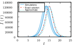
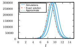
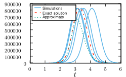
Recently [22] investigated some of the role the distribution of infection duration has on the dynamics of an epidemic. They considered a gamma-distributed infectious period with constant infectiousness. The model they studied corresponds to a chain of exponentially distributed infectious classes, each with infectiousness and expected duration . They showed that the standard SIR equations (1)–(3) provide a poor approximation.
For this system, where . The Laplace transform of this is . From this we can derive the transforms of and , which allows us to define the coefficients for our approximation. Figure 6 shows that the approximation closely follows the early growth even after the exponential phase ends. It finally deviates close to the epidemic peak, but it gives a reasonable estimate of the timing and maximum load of the epidemic.
4 Transition Phase
We have shown that stochastic effects play an important role on whether an epidemic occurs and the timing of an epidemic if it does occur. We have also seen that once the epidemic is sufficiently large, it follows the deterministic predictions. We borrow an approach from [8] to identify when the transition from the stochastic phase to the deterministic phase occurs. For simplicity in our analysis, we will assume that the process is not highly peaked. This allows us to assume that is close to its equilibrium state.
In order to treat the dynamics as deterministic over a time interval , we must satisfy two competing conditions. First, we need the time interval to be large enough that the number of infections and recoveries that happen in that interval is well-approximated by the expected number. That is, we need the expected error to be small compared to the expected value, and so the coefficient of variation (the square root of the variance divided by the expectation) is small. Assuming that the rates remain constant, the infection and recovery processes are both Poisson, and so their difference is a Skellam distribution, which has variance [18, 13]. Consequently the condition we need is that . So
| (17) |
Second, we need the time interval to be small enough that the rate at which the infectious population size changes is not affected by changes in the infectious population. That is we need . So
| (18) |
For small values of , conditions (17) and (18) cannot be satisfied simultaneously.
Combining these conditions we need that
More strictly, we actually require that .
The analysis we have done does not apply close to the peak of the epidemic (where ). Here we can replace condition (17) with the requirement that the error in the number of new infections is small compared to the number of new infections and similarly for the number of recoveries. In general we need condition (18) combined with either this pair of conditions or condition (17) to guarantee that the deterministic equations apply. For practical purposes, once the deterministic equations hold, we expect them to hold through the peak until decays at which point we can use (17) again.
If the generation interval distribution were highly peaked around some typical time, then we could still argue that the system is deterministic, but we would have to explicitly set the history of rather than assuming it is takes the equilibrium form. By assuming the equilibrium distribution we can treat infections as occurring at a slowly changing rate.
5 Discussion
A typical disease outbreak begins small and whether it grows or becomes extinct is strongly influenced by stochastic effects. If it grows, it generally does so faster than predicted deterministically because those outbreaks which are most likely to not die out stochastically are those which initially grow faster than average. Consequently if we observe an epidemic, it is likely to have grown to an epidemic faster than deterministic equations predict.
Once an outbreak becomes large, it transitions to a deterministic phase. We can estimate the size an outbreak must reach to be deterministic by identifying a time interval which is large enough that many events happen in the interval (and so the error of a deterministic prediction is small compared to the prediction), while at the same time the interval is small enough that the size of and do not change significantly. Such a time interval can only exist if is sufficiently large.
Once an outbreak is deterministic, we can use the deterministic equations to accurately model the spread once a correcting time shift is applied. These equations are somewhat difficult because they require saving the history of an epidemic, and so it may be more convenient to use approximate models. We have introduced an approximate model based on standard compartmental models. We assume that the system responds adiabatically to changes in the susceptible fraction. It uses a single infectious class, but has coefficients that change in time. It provides a good estimate of the early behavior, but may deviate close to the peak. We can estimate when it deviates by looking at how quickly the susceptible fraction changes during a typical infectious period.
We have assumed throughout that the infectious population can be modeled in continuous time. If the generation interval is discrete, then these assumptions fail, but similar approaches work in discrete time. A more complicated situation arises when the generation interval distribution is close to discrete: If the distribution is tightly peaked about a mean which is sufficiently far from zero, then it may take many generations for the infectious population to reach equilibrium. The population may become deterministic before the population reaches equilibrium, in which case our exact equations will provide a good model (assuming appropriate initial conditions) while our first approximation may fail badly. Our second approximation may require a long chain of infectious classes in order to reproduce the correct dynamics.
The models we have developed are straightforward to adapt to SIR with birth or death, SIS, or SIRS. In fact, such situations will be more amenable to our first approximating method because the rate of change of is reduced.
Acknowledgments
BP would like to acknowledge the support of Canadian Institutes of Health Research (CIHR) (grants nos. PTL-93146, PAP-93425 and MOP-81273) and the Michael Smith Foundation for Health Research (MSFHR) (Senior Scholar Funds). JCM, BD, and RM were supported by these grants.
JCM was additionally supported by the RAPIDD program of the Science & Technology Directorate, Department of Homeland Security and the Fogarty International Center, National Institutes of Health.
Appendix A Probability Generating Functions
A probability generating function (pgf) is a function which encodes a probability distribution of non-negative integers [23]. Given that the probability of is we define the function
Probability generating functions have a number of useful properties. The product of two pgfs is itself a pgf for the sum of two numbers chosen from each distribution. From this fact, it can be shown that for two pgfs and encoding the distributions and respectively, the function is the pgf for the distribution found by choosing a random number from , and then taking the sum of random numbers from .
This property of function composition is useful in our context to deal with taking a random number of infecteds (corresponding to ), and each of them infects a random number of susceptibles (from a distribution ). The resulting number of new infections is given by the composition of the corresponding pgfs.
A.1 derivation of equations
We assume that the population is sufficiently large relative to the number of infections, that no infections are prevented by depletion of susceptibles. We focus our attention on a single infected individual and its descendants. We can assume that when becomes infected. Let be the time-dependent pgf for the number of individuals (descended from , including ) who are infected at . That is where is the probability that individuals are infected at time .
Let be the pgf for the number of infectious descendants has units of time after becoming infected given that its infection lasts units of time. Note that if , then . Then the number of current infections is given by a weighted average of the number of descendants (plus if is still infectious). Encoding this as a statement for pgfs gives
The number of infections resulting from an individual infected at time has pgf . This allows us to express in terms of .
To find , we consider an individual who recovers at time and divide the duration of infectiousness into small sized blocks. The pgf for the number of infections at time due to an infection that occurs in the interval is . The infection occurs with probability . The probability that infection does not occur during that time period is . Consequently the pgf for the number of infections at time resulting from infections in the time interval of interest is:
The pgf for the number of infections occurring in any of the time intervals is the product of the individual generating functions. Consequently, taking , the pgf for the number of descendants an individual has at time given that it recovers at is
If the individual recovers at time , then the pgf for the number of descendants at time including itself satisfies .
This expression for can be derived alternately by considering a large population size and noting that if the expected number of infections caused by is , then the probability of infecting each individual is The probability of infecting people is then . From this we can derive the pgf for the number of infections caused directly from , and then using function composition will arrive at the same expression.
Appendix B Notes on the numerics for the stochastic problem
We take and where gives the probability of having people infected at time , while gives the probability of having descendants given that recovery occurs at time . If we take derivatives of these equations, divide by and evaluate at , we get the probability of infections. The resulting system of equations is straightforward to solve numerically. As our initial condition at we generally set all derivatives of to be except the first derivative, which is , though other options are possible.
If we make a simplifying assumption that is constant, we can find an expression for which reduces the dimenionality of the problem. We have
We define the auxiliary function . Then
Our equation for remains
This allows us to simplify the calculations by storing at each value of rather than needing to integrate at each time step.
In practice we want to find arbitrary derivatives of evaluated at . To find this numerically, we differentiate these equations with respect to to arrive at equations coupling derivatives of with derivatives of at . Let us assume we know and its derivatives for and and its derivatives. To find and , it is straightforward to use an implicit numerical method.
Appendix C An equivalent formulation
Although equations (6)–(9) are intuitively appealing because of their similarity to the standard SIR equations, we can reduce them to a simpler form. We first replace with . Note that . Further , so from the initial condition at , we can calculate , and have no further need for . Thus we arrive at
| (19) | ||||
| (20) | ||||
| (21) | ||||
| (22) |
If we take as the initial condition that all infections at time begin their infection period at , then for and we can assume that the integrals have their upper limit at . If we take some other initial condition, we may have to include the entire range of . Although these equations are simpler to solve, they lose some of their intuitive appeal because it is more difficult to identify the meaning of each term.
References
- [1] D. Anderson and R. Watson. On the spread of a disease with gamma distributed latent and infectious periods. Biometrika, 67(1):191–198, 1980.
- [2] F. Brauer. Compartmental models in epidemiology. Lecture notes in mathematics: Springer-Verlag, 1945:19, 2008.
- [3] Fred Brauer. Age of infection in epidemiology models. In Electronic Journal of Differential Equations, Conference, volume 12, pages 29–37, 2005.
- [4] R. Breban, R. Vardavas, and S. Blower. Linking population-level models with growing networks: A class of epidemic models. Physical Review E, 72(4):46110, 2005.
- [5] C. Castillo-Chavez, K. Cooke, W. Huang, and SA Levin. On the role of long incubation periods in the dynamics of acquired immunodeficiency syndrome (AIDS). Journal of Mathematical Biology, 27(4):373–398, 1989.
- [6] Kenny Crump and Charles J. Mode. A general age-dependent branching process. II. J. Math. Anal. Appl, 25(1):8–17, 1969.
- [7] Kenny S. Crump and Charles J. Mode. A general age-dependent branching process I. J. Math. Anal. Appl, 24(3):494–508, 1968.
- [8] Daniel T. Gillespie. The chemical Langevin equation. The Journal of Chemical Physics, 113:297, 2000.
- [9] O.P. Gunther, G. Ogilvie, M. Naus, E. Young, D.M. Patrick, S. Dobson, B. Duval, P.A. Noel, F. Marra, D. Miller, et al. Protecting the next generation: What is the role of the duration of human papillomavirus vaccine-related immunity? The Journal of Infectious Diseases, 197(12):1653–1661, 2008.
- [10] P. Haccou, P. Jagers, and V.A. Vatutin. Branching processes: Variation, growth, and extinction of populations. Cambridge University Press, 2005.
- [11] H.W. Hethcote and P. van den Driessche. Two SIS epidemiologic models with delays. Journal of Mathematical Biology, 40(1):3–26, 2000.
- [12] P. Jagers. Branching processes with biological applications. John Wiley & Sons, 1975.
- [13] N.L. Johnson, S. Kotz, and A.W. Kemp. Univariate discrete distributions. Wiley-Interscience, 2005.
- [14] J. Li and F. Brauer. Continuous-time age-structured models in population dynamics and epidemiology. Lecture notes in mathematics: Springer-Verlag, 1945:205, 2008.
- [15] A.L. Lloyd. Destabilization of epidemic models with the inclusion of realistic distributions of infectious periods. Proceedings of the Royal Society B: Biological Sciences, 268(1470):985–993, 2001.
- [16] A.L. Lloyd. Realistic distributions of infectious periods in epidemic models: changing patterns of persistence and dynamics. Theoretical Population Biology, 60(1):59–71, 2001.
- [17] Junling J. Ma and David J. D. Earn. Generality of the final size formula for an epidemic of a newly invading infectious disease. Bulletin of Mathematical Biology, 68(3):679–702, 2006.
- [18] JG Skellam. The frequency distribution of the difference between two Poisson variates belonging to different populations. Journal of the Royal Statistical Society, pages 296–296, 1946.
- [19] Ake Svensson. A note on generation times in epidemic models. Mathematical Biosciences, 208(1):300 – 311, 2007.
- [20] H.R. Thieme and C. Castillo-Chavez. How may infection-age-dependent infectivity affect the dynamics of hiv/aids? SIAM Journal on Applied Mathematics, 53:1447–1447, 1993.
- [21] Jacco Wallinga and Marc Lipsitch. How generation intervals shape the relationship between growth rates and reproductive numbers. Proceedings of the Royal Society B: Biological Sciences, 274(1609):599–604, 2007.
- [22] H.J. Wearing, P. Rohani, and M.J. Keeling. Appropriate models for the management of infectious diseases. PLoS Medicine, 2(7):e174, 2005.
- [23] Herbert S. Wilf. generatingfunctionology. A K Peters, Ltd, 3rd edition, 2005.