Dimension reduction and variable selection in case control studies
via regularized likelihood optimization

Abstract.

Dimension reduction and variable selection are performed routinely in case-control studies, but the literature on the theoretical aspects of the resulting estimates is scarce. We bring our contribution to this literature by studying estimators obtained via $\ell_{1}$ penalized likelihood optimization. We show that the optimizers of the $\ell_{1}$ penalized retrospective likelihood coincide with the optimizers of the $\ell_{1}$ penalized prospective likelihood. This extends the results of Prentice and Pyke (1979), obtained for non-regularized likelihoods. We establish both the sup-norm consistency of the odds ratio, after model selection, and the consistency of subset selection of our estimators. The novelty of our theoretical results consists in the study of these properties under the case-control sampling scheme. Our results hold for selection performed over a large collection of candidate variables, with cardinality allowed to depend and be greater than the sample size. We complement our theoretical results with a novel approach of determining data driven tuning parameters, based on the bisection method. The resulting procedure offers significant computational savings when compared with grid search based methods. All our numerical experiments support strongly our theoretical findings.

1. Introduction

Case-control studies investigate the relationship between a random outcome $Y$, typically the disease status, and a number of candidate variables $X_{j}$, $1\leq j\leq M$, that are potentially associated with $Y$. An important instance is provided by cancer studies, where the $X_{j}$’s may quantify exposures to certain substances, or may be a collection of genes or genetic markers. One of the problems of interest in such studies is the identification, on the basis of the observed data, of a smaller subset of the set of candidate variables, that can reliably suffice for subsequent analyses. This problem becomes more challenging when the collection of potential disease factors $M$ is very large. Our solution to this problem is variable selection via penalized likelihood optimization. We propose below a computationally efficient selection method and we investigate the theoretical properties of our estimates under the case-control data generating mechanism. We begin by giving the formal framework used throughout the paper and by making our objectives precise.

We consider binary outcomes $Y\in\{0,1\}$, where $Y=0$ labels the controls (non-disease), and $Y=1$ labels the cases (disease). Let $f_{0}(x),f_{1}(x)$ be, respectively, the conditional distributions of $X=(X_{1},\ldots,X_{M})$ given $Y=0$ and $Y=1$. Under the case-control or retrospective sampling scheme we observe two independent samples from each of these conditional distributions. Formally, we observe

(1.1) $$X_{1}^{0}\ldots,X_{n_{0}}^{0}\ \mbox{i.i.d. with density}\ f_{0}(x),$$

$$X_{1}^{1}\ldots,X_{n_{1}}^{1}\ \mbox{i.i.d. with density}\ f_{1}(x),$$

where the superscripts 0 and 1 of $X$ are mnemonic of the fact that the samples correspond to $Y=0$ and $Y=1$, respectively. For simplicity of notation we assume that $n_{0}=n_{1}=n$. We assume that the outcome $Y$ is connected to $X$ via the logistic link function

(1.2) $$P(Y=1|X=x)=\frac{\exp{(\delta_{0}+\beta^{\prime}x)}}{1+\exp(\delta_{0}+\beta^{\prime}x)},$$

where $\beta\in\mathbb{R}^{M}$, $\delta_{0}\in\mathbb{R}$.

In this article we will further assume that $\beta=\beta^{*}$, where $\beta^{*}\in\mathbb{R}^{M}$ has non-zero components corresponding to an index set $I^{*}\subseteq\{1,\ldots,M\}$ with cardinality $|I^{*}|=k^{*}$, possibly much smaller than $M$. The variable selection problem can be therefore rephrased in this context as the problem of estimating the unknown set $I^{*}$ from data generated as in (1.1). We note that this problem is not equivalent with the problem of estimating $I^{*}$ from i.i.d. pairs $(X_{i},Y_{i})$, with $Y_{i}$ generated from (1.2), as no random samples from the distribution of $Y$ are available under the sampling scheme (1.1). However, the likelihoods corresponding to the two sampling schemes are intimately related, with results detailing their connections dating back to the 1970s. This link is essential for our procedure and we illustrate it below. Following Prentice and Pyke (1979), Section 3, an application of the Bayes’ theorem combined with rearranging terms gives the following re-parametrization of $f_{0}$ and $f_{1}$, respectively:

(1.3) $$f_{0}(x) = 2\times\frac{1}{1+\exp(\delta+\beta^{\prime}x)}\times q(x)=:2p_{0}(x)q(x),$$

$$f_{1}(x) = 2\times\frac{\exp(\delta+\beta^{\prime}x)}{1+\exp(\delta+\beta^{\prime}x)}\times q(x)=:2p_{1}(x)q(x),$$

where $\delta$ is a new intercept parameter, different than $\delta_{0}$, $\beta$ is given by (1.2), and $q(x)$ is a positive function that integrates to one. The parameters $\delta$, $\beta$ and $q$ are constrained by the requirement that $f_{0}$ and $f_{1}$ are probability densities, that is

(1.4) $$\int p_{j}(x)q(x)dx=\frac{1}{2};\ \ j\in\{0,1\}.$$

Therefore, the likelihood function corresponding to data generated as in (1.1), to which we will refer in the sequel as to the retrospective likelihood, is:

$$L_{retro}(\delta,\beta,q) =: \Pi_{i=1}^{n}f_{0}(x_{i}^{0})f_{1}(x_{i}^{1})$$

$$= \left\{\Pi_{i=1}^{n}p_{0}(x_{i}^{0})p_{1}(x_{i}^{1})\right\}\times\left\{4\Pi_{i=1}^{n}q(x_{i}^{0})q(x_{i}^{1})\right\}$$

$$=: L_{pros}(\delta,\beta)\times L(q),$$

with parameters $\delta,\beta$ and $q$ related via the constraint (1.4). Notice that $L_{pros}$ is, up to the intercept, exactly the standard logistic regression likelihood, had we observed $2n$ i.i.d observations $(X_{i},Y_{i})$, with equal number of 0 and 1 responses $Y_{i}$ generated according to (1.2); this quantity and the corresponding sampling scheme are typically referred to in this context as the prospective likelihood, and prospective sampling scheme, respectively. We will also use this terminology below.

The earlier results on the estimation of $\beta$ via (1) did not address the model selection problem and were mostly concerned with the asymptotic properties of the estimates of $\beta$. Anderson (1972), Prentice and Pyke (1979), Farewell (1979) are among the pioneers of this work and showed that:

(1) The vector $\tilde{\beta}\in\mathbb{R}^{M}$ that maximizes the retrospective likelihood $L_{retro}(\delta,\beta)$ under the constraint (1.4) coincides with $\bar{\beta}\in\mathbb{R}^{M}$ that maximizes the prospective likelihood $L_{pros}(\delta,\beta)$;

(2) The asymptotic distribution of $\tilde{\beta}$, derived under the sampling scheme (1.1) coincides with the asymptotic distribution of $\bar{\beta}$ derived under the prospective sampling scheme.

A number of important works continued this program, and provided in depth analyses of various other aspects of the estimators of $\beta$ in retrospective studies. We refer to Gill, Vardi and Wellner (1988) and Carroll, Wang and Wang (1995), for more general sampling schemes, to Qin and Zhang (1997) for goodness of fit tests, to Breslow, Robins and Wellner (2000) for a study of the efficiency of the estimators, to Murphy and van der Vaart (2001), for partially observed covariates, to Osius (2009), for general semiparametric association models and to Chen, Chatterjee and Carroll (2009), for shrinkage methods tailored to inference in haplotype-based case-control studies and the asymptotic distribution of the resulting estimators. The variable selection problem was not considered in any of these works. Although model selection techniques are routinely used in case-control studies, and are typically based on testing via the asymptotic distribution of $\widehat{\beta}$, we are unaware of theoretical analyses of the performance of the resulting estimators under this sampling scheme.

Our contribution to this literature is to provide answers to the model selection analogues of (1), and to formulate goals that replace (2) above by goals targeted to the dimension reduction and selection aspects. Specifically, we propose a model selection method based on a penalized likelihood approach, with a sparsity inducing penalty. In this article we will focus on the $\ell_{1}$ penalized likelihood with tuning parameter $\lambda$. We will show the following:

(I) For any penalty function $pen(\beta)$ that is independent of $\delta$, the maximizer of $L_{retro}(\delta,\beta)+pen(\beta)$ under the constraint (1.4) coincides with the maximizer of the prospective likelihood $L_{pros}(\delta,\beta)+pen(\beta)$.

(II) For $pen(\beta)=\lambda\sum_{j=1}^{M}|\beta_{j}|$, we obtain estimators $\hat{I}$ of $I^{*}$ and dimension reduced estimators $\widehat{\beta}$ of $\beta^{*}$ by optimizing $L_{pros}(\delta,\beta)+pen(\beta)$. Then:

(a) The behavior of $\mathbb{P}(\widehat{I}=I^{*})$, analyzed under the sampling scheme (1.1) is essentially the same as the behavior of $\mathbb{P}(\widehat{I}=I^{*})$, evaluated under the prospective sampling schemes.

(b) The estimator $\widehat{\beta}$, analyzed under the sampling scheme (1.1), adapts to the unknown sparsity of $\beta^{*}$, which parallels the same property that can be established for $\widehat{\beta}$, under the prospective sampling schemes.

The result announced in (I) is an immediate extension of result (1) above established in the 1970s for the unpenalized likelihood. We present it in Section 2 below. The results in (II) necessitate an analysis that is completely different than the one needed for (2), and we discuss (a) in Section 4 and (b) in Section 3. The immediate implication of (b) that is relevant to case-control studies is the fact that the estimator $\widehat{\beta}$, which is supported on a space of potentially much lower dimension than the original $\mathbb{R}^{M}$, yields sup-norm consistent estimates of the odds ratio, where the odds ratio is defined as follows. The odds of having $Y=1$ for an individual with characteristics $X=x$ are $O(x)=P(Y=1|X=x)/P(Y=0|X=x)$, and the odds ratio is defined as $O(x)/O(x_{0})$, for some reference characteristic $X=x_{0}$. Under model (1.2), the odds ratio becomes

(1.6) $$R(x)=:\exp(\beta^{{}^{\prime}}(x-x_{0})).$$

We establish the after model selection consistency of estimators of this ratio in Section 3 below.

In this article we will concentrate on the analysis of estimators obtained by optimizing $\ell_{1}$ penalized criteria. The literature on the theoretical aspects of such estimates has seen an explosion in the past few years, together with the development of efficient algorithms for computing them. The results pertaining to generalized linear models are most closely connected to our work, and all of them have been established for what we termed above the prospective sampling scheme, that is for data consisting of $(X_{i},Y_{i})$ i.i.d. pairs. For analyses conducted under this framework, we refer to van der Geer (2008) and Bunea (2008), for sparsity oracle inequalities for the Lasso, and to Bunea (2008), for correct subset selection; we refer to Ravikumar, Wainwright and Lafferty (2008) for related results on graphical models for binary variables. Motivated by the increasing usage of the Lasso type estimators for the analysis of data arising from case-control studies, see e.g., Shi, Lee and Wahba (2007), Wu et al (2009) and the references therein, we complement the existing literature on this type of estimators by providing their theoretical analysis under the case-control data generating mechanism (1.1). To the best of our knowledge, this is the first such analysis proposed in the literature.

The rest of the paper is organized as follow. Section 5 complements the theoretical results of Sections 2 - 4, by providing a fast algorithm for finding a data driven tuning parameter for the $\ell_{1}$ penalized optimization problem. Our procedure does not use a grid search. Instead, we use a generalization of the bisection method to compute tuning parameters that yield, respectively, estimators with exactly $k=0,1,\dots,M$ non-zero components. We then use a 10-fold cross-validated logistic loss function to which we add a BIC-type penalty to select one of these estimators. The corresponding procedure is easy to implement and offers important computational savings over a grid search based procedure, which can be 50 times slower, for the same degree of accuracy. Section 6 contains a detailed analysis of the proposed estimators, via simulations. It supports very strongly all our theoretical findings. Section 7 is a conclusion section, summarizing our findings. All the proofs are collected in the Appendix.

2. Penalized logistic regression for case-control data

In this section we investigate the type of penalty functions for which estimation of $\beta$ via penalized retrospective log-likelihood optimization reduces to the estimation of $\beta$ via penalized prospective likelihood optimization. Recall that we mentioned in (1) above that the retrospective likelihood can be written as the product of the prospective likelihood and a term depending on $q$:

$$L_{retro}(\delta,\beta,q) =: L_{pros}(\delta,\beta)\times L(q),$$

where the parameters $\delta$, $\beta$ and $q$ are constrained by (1.4). Let $pen(\beta)$ be a function that depends on $\beta$ alone, and is independent of $\delta$ and $q$. Define the unconstrained maxima

(2.1) $$(\widehat{\delta},\widehat{\beta})=\mathop{\rm arg\,max}_{\delta,\beta}\left\{\log L_{pros}(\delta,\beta)+pen(\beta)\right\};\ \ \ \widehat{q}=\mathop{\rm arg\,max}_{q}\log L(q),$$

where the second maximum is taken over all density functions $q$. The following result, proved in the Appendix, is an immediate extension of the result derived by Prentice and Pike (1979) for the unpenalized likelihood.

Lemma 2.1.

Let $pen(\beta)$ be any function independent of $\delta$ and $q$. Let $\widehat{\delta},\widehat{\beta}$ and $\widehat{q}$ be given by (2.1). Then

$$((\widehat{\delta},\widehat{\beta}),\widehat{q})=\mathop{\rm arg\,max}_{\delta,\beta,q}\{\log L_{retro}(\delta,\beta,q)+pen(\beta)\},$$

where the maximizer is computed over all $\delta,\beta,q$ satisfying the constraint (1.4).

Lemma 2.1 shows that the penalized log-likelihood estimates of $(\delta,\beta$), for a likelihood corresponding to data generated as in (1.1) coincide with the penalized prospective log-likelihood estimates, which we rescale by $2n$:

$$(\widehat{\delta},\widehat{\beta}) = \mathop{\rm arg\,min}_{\delta,\beta}\{-\frac{1}{2n}\log L_{pros}(\delta,\beta)+pen(\beta)\}$$

$$=: \mathop{\rm arg\,min}_{\delta,\beta}(\frac{1}{2n}\sum_{i=1}^{n}\log(1+e^{\delta+\beta^{\prime}{X}_{i}^{1}})-\frac{1}{2n}\sum_{i=1}^{n}(\delta+\beta^{\prime}{X}_{i}^{1})$$

$$+\frac{1}{2n}\sum_{i=1}^{n}\log(1+e^{\delta+\beta^{\prime}{X}_{i}^{0}})+pen(\beta)).$$

Lemma 2.1 holds for any function $pen(\beta)$, as long as it is independent of $\delta$ and $q$. Since we are interested in dimension reduction, we will consider a sparsity inducing penalty. Throughout this paper our estimates will be obtained via (2) with the $\ell_{1}$ penalty given below

(2.3) $$pen(\beta)=\lambda\sum_{j=1}^{M}|\beta_{j}|,$$

for a tuning parameter $\lambda$ that will be made precise in the following section.

3. Consistent estimation of the odds ratio
after variable selection

Recall that the true odds ratio (1.6) is given in terms of $\beta^{*}$, which is supported on a space of dimension $k^{*}$, possibly much smaller than $M$. We show that the estimated odds ratio based on the selected variables corresponding to the non-zero elements of $\widehat{\beta}$ given by (2) above, for penalty (2.3), provides a consistent estimate, in the supremum norm, of the odds ratio:

(3.1) $$\sup_{x}|\exp\widehat{\beta}^{\prime}(x-x_{0})-\exp{\beta^{*}}^{\prime}(x-x_{0})|\longrightarrow 0,$$

with probability converging to one. For simplicity of notation, we assume in what follows that $x_{0}=0$. For uniformity of notation, we also denote the intercept parameter given in (1.3) by $\delta^{*}$.

Our arguments are based on the following central fact, that may be of independent interest. Define the functions

$$\ell_{0}(\theta) =: \ell_{0}(\theta;x)\ =\ \log(1+e^{\theta^{\prime}x}),$$

$$\ell_{1}(\theta) =: \ell_{1}(\theta;x)\ =\ \log(1+e^{\theta^{\prime}x})-\theta^{\prime}x,$$

and recall the notation $\theta=(\delta,\beta)$. In order to write what follows in a compact way we further denote by $\mathbb{P}^{0}$ and $\mathbb{P}^{1}$ the probability measures corresponding to the densities $f_{0}$ and $f_{1}$ defined in (1.3), respectively. For a generic function $g$ we write $\mathbb{P}^{0}g$ and $\mathbb{P}^{1}g$ for integration with respect to $\mathbb{P}^{0}$ and $\mathbb{P}^{1}$, respectively. With this notation we define the quantity

(3.2) $$\Delta(\widehat{\theta},\theta^{*})=\frac{1}{2}\mathbb{P}^{0}\left(\ell_{0}(\widehat{\theta})-\ell_{0}(\theta^{*})\right)+\frac{1}{2}\mathbb{P}^{1}\left(\ell_{1}(\widehat{\theta})-\ell_{1}(\theta^{*})\right).$$

Theorem 3.1 below, which is central to our paper, establishes that the difference $\Delta$ is small. The proof, given in the Appendix, uses the control of appropriately scaled empirical processes corresponding to the two samples. If $\Delta\left((\widehat{\delta},\widehat{\beta}),(\delta^{*},\beta^{*})\right)$ is small with high probability, relatively standard arguments can be used to show that

$$\sup_{x}|\widehat{\beta}^{\prime}x-\beta^{*\prime}x+\widehat{\delta}-\delta^{*}|$$

is also small, with high probability, and we establish this in Corollary 3.2 below.

To arrive at our desired result (3.1), we need to complement Corollary 3.2 with a study of the difference $|\widehat{\delta}-\delta^{*}|$. This is done in Theorem 3.3, which also contains a stronger result: it shows that $\widehat{\beta}$ adapts to the unknown sparsity of $\beta^{*}$, in that it is a consistent estimator of $\widehat{\beta}$, with the rate of convergence of an estimate based only on $I^{*}$ variables.

The combination of Theorem 3.1, Corollary 3.2 and Theorem 3.3 yields the desired sup-norm consistency of the odds ratio stated in Theorem 3.4. All proofs are collected in the Appendix. All our theoretical results will be proved under the assumption that the design variables and the true parameter components are bounded. We formalize this in Assumption 1 below.

Assumption 1.

(i) There exits a constant $L>0$, independent of $M$ and $n$, such that $|X_{i}^{j}|\leq L$, for all $i$ and $j$, with probability 1.

(ii) There exits a constant $B>0$, independent of $M$ and $n$, such that $\max_{j}|\beta_{j}^{*}|\leq B$; $|\delta^{*}|\leq B.$

Let $\delta_{n}$ be any sequence converging to zero with $n$. Define the tuning sequence

(3.3) $$r=\log n\left(6L\sqrt{\frac{2\log 2(M\vee n)}{n}}+\frac{1}{4(M\vee n)}+4L\sqrt{\frac{2\log\frac{1}{\delta_{n}}}{n}}\right).$$

If $\delta_{n}=1/n$ and $M$ is polynomial in $n$, the tuning sequence $r$ is of the order $\frac{\log n\sqrt{\log n}}{\sqrt{n}}$. The results of this section will be relative to estimators obtained via the penalty (2.3), with tuning parameter $\lambda=2r$. For compactness of notation, we let $\widehat{\theta}=:(\widehat{\delta},\widehat{\beta})\in\mathbb{R}^{M+1}$,  $\theta^{*}=:(\delta^{*},\beta^{*})\in\mathbb{R}^{M+1}$. Whenever we use this compact notation, we will also use the notation $\widehat{\theta}^{\prime}u$ or ${\theta^{*}}^{\prime}u$, for some vector $u\in\mathbb{R}^{M+1}$ that will be implicitly assumed to have the first component equal to 1.

Theorem 3.1.

Under Assumption 1, if $k^{*}r\rightarrow 0$, then for any $\alpha>0$

$$\mathbb{P}(\Delta(\widehat{\theta},\theta^{*})>\alpha)\longrightarrow 0,$$

as $n\rightarrow\infty$.

We give an immediate corollary of this theorem which establishes the sup-norm consistency of $\widehat{\theta}^{\prime}x$. It is interesting to note that both Theorem 3.1 above and the corollary below hold under no assumptions on the dependence structure of the design variables.

Corollary 3.2.

Under Assumption 1, if $k^{*}r\rightarrow 0$, then for any $\gamma>0$

$$\mathbb{P}\left(\sup_{x}|(\widehat{\beta}^{\prime}{x}-{\beta}^{*\prime}{x})+(\widehat{\delta}-\delta^{*})|\geq\gamma\right)\longrightarrow 0,$$

as $n\rightarrow\infty$.

The following theorem establishes rates of convergence for the estimates of $\delta^{*}$ and $\beta^{*}$. It requires minimal conditions on the design variables. We formalize them below. Let $V$ be a $(M+1)\times(M+1)$ matrix containing a $(k^{*}+1)\times(k^{*}+1)$ identity matrix, corresponding to $I^{*}$ and the intercept, and with zero elements otherwise. Let $X_{1},\ldots,X_{n}$ denote $X_{1}^{0},\ldots,X_{n}^{0}$, and let $X_{n+1},\ldots,X_{2n}$ denote $X_{1}^{1},\ldots,X_{n}^{1}$. By convention, each $X_{i}$ is viewed as a vector in $\mathbb{R}^{M+1}$ with the first component equal to 1, i.e. $X_{0i}=1$, for all $i$. We used this compact notation to avoid unnecessary superscripts. Let $\Sigma$ be the $(M+1)\times(M+1)$ sample Hessian matrix with entries

$$\frac{1}{2n}\sum_{i=1}^{2n}p_{0}(X_{i})p_{1}(X_{i})X_{ki}X_{ji},\ 0\leq j,k\leq M.$$

Condition H. There exists $0<b\leq 1$ such that $\mathbb{P}(\Sigma-bV\geq 0)=1$.

Remark. Condition H is a mild condition on $\Sigma$, as it requires that this matrix remain semi-positive definite after a slight modification of some of its diagonal elements, those corresponding to $I^{*}$. This relaxes the conditions needed for the consistency of the estimators based on the non-regularized log-likelihood, when one requires that the Hessian matrix be positive definite, see e.g. Prentice and Pyke (1979).

Let $c=6/bw$, for $b$ given by Condition H above and for some positive number $w$ that is arbitrarily close to 1.

Theorem 3.3.

Under Assumption 1 and Condition H, if $k^{*}r\rightarrow 0$, then

$$(i)\ \ \mathbb{P}\biggl{(}|\widehat{\delta}-\delta^{*}|\leq crk^{*}\biggr{)}\longrightarrow 1,$$

$$(ii)\ \ \mathbb{P}\biggl{(}\sum_{j=1}^{M}|\widehat{\beta}_{j}-\beta_{j}^{*}|\leq crk^{*}\biggr{)}\longrightarrow 1,$$

as $n\rightarrow\infty$.

The theorem shows that the rate of convergence of $\widehat{\beta}$ adapts to the unknown sparsity of $\beta^{*}$: $\sum_{j=1}^{M}|\widehat{\beta}_{j}-\beta_{j}^{*}|$ has $M$ terms, so we expect its size to be equal to the optimal rate $1/\sqrt{n}$ of each term multiplied by $M$. Theorem 3.3 shows that in fact $\widehat{\beta}$ behaves like an estimator obtained in dimension $k^{*}$, had this dimension been known, as its rate of convergence in the $\ell_{1}$ norm is, up to constants and logarithmic terms, $1/\sqrt{n}$ multiplied by $k^{*}$, for our choice of $r$.

Theorem 3.3 is the result announced in II(b) of the introduction: the estimators of $\beta^{*}$ analyzed under the retrospective sampling scheme exhibit the same adaptation to sparsity as those analyzed under the prospective sampling scheme. For a full analysis of the $\ell_{1}$ penalized logistic regression estimates based on i.i.d. $(X_{i},Y_{i})$ pairs, with $Y_{i}$ generated as in (1.2) we refer to Bunea (2008), for results obtained under conditions similar to Condition H on the Hessian matrix, and to van de Geer (2008), for results on generalized linear models obtained under conditions on the covariance matrix of the covariates. The difference between the results obtained under the two sampling schemes is essentially minor, and consists in a slight difference in the size of the tuning parameter $r$, which needs to be larger, by a $\log n$ factor, for the case control studies. This is a very small price to pay for not having full information on the joint distribution of $X$ and $Y$.

Corollary 3.2 and Theorem 3.3 (i) immediately imply, via a first order Taylor expansion, the desired result of this section. We summarize it in Theorem 3.4 below which shows that for appropriate choices of the tuning parameters $r$, and if the size of the true model does not grow very fast relative to $1/r$ then, under minimal conditions on the covariates, we can estimate the odds ratio consistently.

Theorem 3.4.

Under Assumption 1 and Condition H, if $k^{*}r\rightarrow 0$, then

$$\mathbb{P}(\sup_{x}|\hat{R}(x)-R(x)|\leq\alpha)\longrightarrow 1,$$

for any $\alpha>0$, as $n\rightarrow\infty$.

4. Consistent variable selection

In this section we investigate the consistency of the index set $\widehat{I}$ corresponding to the non-zero components of the estimator $\widehat{\beta}$ discussed above. We show that $\mathbb{P}(I^{*}=\hat{I})\longrightarrow 1$ holds for the retrospective scheme, under conditions similar to those needed in the prospective sampling scheme. We state them below.

Condition 1.  There exists $d>0$ such that

$$\mathbb{P}\Bigg{(}\max_{j\in I^{*},k\neq j}\Bigg{|}\frac{1}{2n}\sum_{i=1}^{2n}X_{ij}X_{ik}\Bigg{|}\leq\frac{d}{k^{*}}\Bigg{)}=1.$$

For $p_{0}$ and $p_{1}$ defined in (1.3) above, we assume that the following also holds.

Condition 2.  There exits $d>0$ such that

$$\mathbb{P}\Bigg{(}\max_{j\in I^{*},k\neq j}\Bigg{|}\frac{1}{2n}\sum_{i=1}^{2n}p_{0}(X_{i})p_{1}(X_{i})X_{ij}X_{ik}\Bigg{|}\leq\frac{d}{k^{*}}\Bigg{)}=1.$$

Remark 1. The constants $d$ in the two conditions above need not be the same; we used the same letter for clarity of notation. Remark 2. The two conditions above can be regarded as conditions guaranteeing the identifiability of the set of true variables $I^{*}$. Condition 1 requires that there exists some degree of separation between the variables in $I^{*}$ and the rest, in that the correlations between variables in these respective sets are bounded, up to constants, by $1/k^{*}$. If $k^{*}$ is small to moderate, the restriction is mild. Condition 2 reinforces Condition 1, by requiring that these variables remain separated even when separation is measured by the entries in the Hessian matrix, which can be regarded as weighted correlations.

Let $\delta_{n}$ be any sequence converging to zero with $n$. Define the tuning sequence

(4.1) $$r=\log n\left(6L\sqrt{\frac{2\log 2(M\vee n)}{n}}+\frac{1}{4(M\vee n)}+4L\sqrt{\frac{2\log\frac{M}{\delta_{n}}}{n}}\right),$$

and notice that the last term in this definition of $r$ differs by a factor of $\sqrt{\log M}$ from the last term in $r$ given in (3.3) of the previous section. If $\delta_{n}=1/n$ and $M$ is polynomial in $n$, the tuning sequence is again of the order $\frac{\log n\sqrt{\log n}}{\sqrt{n}}$. The following assumption reflects the fact that we can only detect coefficients above the noise level, as quantified by $r$.

Assumption 2. $\min_{j\in I^{*}}|\beta_{j}^{*}|>4r$.

Theorem 4.1.

Under Assumptions 1 and 2, if $k^{*}r\rightarrow 0$ and Conditions 1 and 2 are met, then $\mathbb{P}(I^{*}=\hat{I})\longrightarrow 1,$ as $n\rightarrow\infty$.

Theorem 4.1 shows that $\widehat{I}$, analyzed under the retrospective sampling scheme, is a consistent estimator of $I^{*}$, under essentially the same conditions needed for its analysis under the prospective sampling scheme, see Bunea (2008) and also Ravikumar, Wainwright and Lafferty (2008) for related results.

5. Data based tuning sequences and the bisection method

In Sections 3 and 4 above we showed that if the cardinality of the true model is not larger than $\sqrt{n}$, up to constants, the proposed method yields consistent estimation of the odds ratio and of the support of $\beta^{*}$, for tuning sequences $r$ given in (3.3) and (4.1), respectively. Since the constants involved in these expressions may be conservative, we complement our theoretical results by offering in this section a fully data driven construction of the tuning parameters. Typical methods involve two main steps. In the first step one computes the regularization path of the solution to (2), as the tuning parameter $r$ varies. Then, in a second step, one selects the appropriate value of $r$ from a fine grid of values, by cross-validating the log-likelihood.

We present here a method that follows in spirit this idea, but with two main modifications: we do not need to compute the regularization path, but rather a sketch of it and we choose $r$ via a combined cross-validation/BIC -type procedure. We describe the resulting technique in what follows.

We begin by noting that, unlike $\ell_{1}$ penalized least squares, the regularization path for the $\ell_{1}$ penalized logistic likelihood is not piecewise linear and it cannot be computed analytically, see e.g., Rosset and Zhu (2007), Koh et al. (2007). In this case, approximate regularization paths can be obtained from path following algorithms, see, e.g., Hastie et al. (2004), Park and Hastie (2006, 2007), Rosset (2005). These constructions rely on the following observation: the values of the tuning parameter $r$ define a partition of the positive axis, such that for all $r$ belonging to an interval of this partition we obtain the same sparsity pattern. Thus, the full information on the sparsity pattern can be recovered from having a representative inside each such interval.

We call the path corresponding to these representative values a ”sketch” of the regularization path. The problem therefore reduces to finding the set of representatives. For this, one could perform a grid search and find the intervals where the sparsity pattern change. However, a grid search method may not include some of these intervals, as they can have arbitrary length. Thus, a grid search may skip some of the sparsity patterns that are in fact present in the regularization path. Figure 1 below offers an instance of this fact.

Figure 1. Approximate regularization path for normal iid data, $2n=300$, $M=15$ and $k^{*}=3$. Left: the regularization path sketch of $\widehat{\beta}$, obtained using GBM. Right: regularization path of $\widehat{\beta}$ using a grid search with the same computational complexity as the GBM.

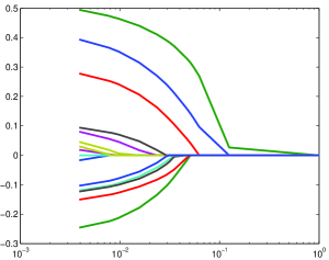
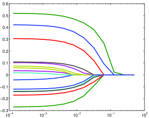
It shows that a grid search with the same computational complexity as the generalized bisection method GBM, described in detail below, can fail to contain the true index set $I^{*}$ in the corresponding regularization path. In this example $I^{*}$ has three elements, which can be recovered in the left panel, and not in the right panel, as there is no value of $r$ in the grid we considered for which we can have exactly three non-zero components.

Our procedure replaces the grid search with a different method, that allows us to obtain, for each dimension $1\leq k\leq M$, a value of $r$ for which the solution given by (2) has exactly $k$ non-zero components. For each tuning parameter $r$, let the number of nonzero entries in $\hat{\beta}_{r}$ be denoted by $\hat{n}(r)$. For each dimension $1\leq k\leq M$ we let $h_{k}(r)=\hat{n}(r)-k$. Our method consists in finding $r$ such that $h_{k}(r)=0$. To solve this equation we use the Bisection Method, e.g. Burden and Faires (2001), which is a well established computationally efficient method for finding a root $z\in\mathbb{R}$ of a generic function $h(z)$. The bisection method can be summarized as follows. Let $\alpha$ be the desired degree of accuracy of the algorithm.

The Basic Bisection Method (BBM).
Given $\alpha>0$, do:

1. Choose $z_{0},z_{1}$ such that $h(z_{0})h(z_{1})\leq 0$ (i.e. $h(z_{0}),h(z_{1})$ have different signs).

2. If $h(z_{0})=0$ or $h(z_{1})=0$ stop.

3. Take $z=(z_{0}+z_{1})/2$. If $|z_{1}-z_{0}|<\alpha$ then stop and return $z$.

4. If $h(z)h(z_{0})<0$, make $z_{1}=z$.

5. Else $h(z)h(z_{1})<0$ and make $z_{0}=z$.

6. Return to step 3.

We can apply the basic bisection method to solve $h_{k}(r)=0$, for each $k$, and obtain the desired values of the tuning sequence $r_{1},\ldots,r_{M}$. However, performing BBM for each dimension $k$ separately is not computationally efficient, as there is a large amount of overlapped computation. In what follows we propose an extension of the BBM that finds a sequence $r_{0},...,r_{M}$ such that $\hat{n}(r_{k})=k$, for all $0\leq k\leq M$. The extension uses a queue consisting of pairs $(r_{i},r_{j})$ such that $\hat{n}(r_{i})<\hat{n}(r_{j})-1$.

The General Bisection Method for all $k$ (GBM).
Initialize all $r_{i}$ with $-1$.

1. Choose $r_{0}$ very large, such that $\hat{n}(r_{0})=0$. Choose $r_{n}=0$, hence $\hat{n}(r_{n})=n$.

2. Initialize a queue $q$ with the pair $(r_{0},r_{n})$.

3. Pop the first pair $(a,b)$ from the queue.

4. Take $r=(a+b)/2$. Compute $k=\hat{n}(r)$.

5. If $r_{k}=-1$ make $r_{k}=r$.

6. If $|\hat{n}(a)-k|>1$ and $|a-r|>\alpha$, add $(a,r)$ to the back of the queue.

7. If $|\hat{n}(b)-k|>1$ and $|b-r|>\alpha$, add $(r,b)$ to the back of the queue.

8. If the queue is not empty, go to 3.

The GBM described above offers a way of obtaining candidate values $r_{0},\ldots,r_{M}$ for the tuning parameter $r$. Observe that this method does not use anything specific to the $\ell_{1}$-regularized logistic loss function. The GBM can be used in connection with any penalized loss function, for a sparsity inducing penalty. This makes the GBM method more general than the one proposed in Park and Hastie (2007), which is restricted to $\ell_{1}$- regularized generalized linear models.

We performed a quantitative evaluation of the GBM on four problems of different difficulty levels. The data were simulated from a Normal distribution, described in Section 6 below as NOR_IID. In Table 1 below we compared the GBM and a grid search in terms of their capability of constructing approximate regularization paths containing the true $I^{*}$. The percentages reported in the table are percentages of time $I^{*}$ was in the path, over 250 simulations. Table 1 indicates that if the set $I^{*}$ is in the regularization path, it will also be in the GBM path sketch, obtained at a low computational expense.

Experiment	Size $2n$	$k^{*}=|I^{*}|$	GBM	Grid	Grid$\times$10	Grid$\times$50
1	100	3	70.0	28.8	64.8	70.0
2	200	3	99.2	79.2.7	99.2	99.2
3	300	10	88.4	76.8	87.2	87.6
4	400	10	98.8	93.2	98.8	98.8

Table 1. Percentage of times the $I^{*}$ was present in different approximate regularization paths for the Normal dataset NOR_IID, $M=250$. Grid has the same computational complexity as the GBM, while Grid$\times$10 and Grid$\times$50 are finer grids that are $10$ respectively $50$ times more expensive than the GBM.

To complete the selection procedure, we use the dimension stabilized $p$-fold cross-validation procedure summarized below. Let $D$ denote the whole data set, and let $D=D_{1}\cup\ldots\cup D_{p}$ be a partition of $D$ in $p$ disjoint subsets, each subset containing the same percentage of cases and controls. In all the experiments presented in the next section we took $p=10$. Let $D_{-j}=D\setminus D_{j}$. We will denote by $r_{k}^{j}$ a candidate tuning parameter determined using the GBM on $D_{-j}$. We denote by $I_{k}^{j}$ the set of indices corresponding to the non-zero coefficients of the estimator of $\beta$ given by (2), for tuning parameter $r_{k}^{j}$ on $D_{-j}$. We denote the unpenalized maximum likelihood estimators corresponding only to the variables with indices in $I_{k}^{j}$ and computed on $D_{-j}$ by $(\hat{\delta}^{j},\hat{\beta}_{k}^{j})$. With $\log L_{pros}(\delta,\beta)$ defined in (2) above, let $L_{k}^{j}=:\log L_{pros}(\hat{\delta}^{j},\hat{\beta}_{k}^{j})$, computed on $D_{j}$. With this notation, the procedure becomes: Variable Selection Procedure.
Given: a dataset $D$ partitioned into $p$ disjoint subsets: $D=D_{1}\cup\ldots\cup D_{p}$, each subset containing the same percentage of cases and controls. Let $D_{-j}=D\setminus D_{j}$ for all $j$.

1. For each $1\leq k\leq M$ and each fold $j$ of the partition, $1\leq j\leq p$:
   Use the GBM to find $r_{k}^{j}$ and $I_{k}^{j}$ such $\hat{n}(r_{k}^{j})=|I_{k}^{j}|=k$ on $D_{-j}$.
   Compute $L_{k}^{j}=:\log L_{pros}(\hat{\delta}^{j},\hat{\beta}_{k}^{j})$, as defined above.

2. For each $1\leq k\leq M$:
   Compute $L_{k}=:\frac{1}{p}\sum_{j=1}^{p}L_{k}^{j}$.

3. Obtain

   $$\hat{k}=\mathop{\rm arg\,min}_{k}(L_{k}+0.5k\frac{\log 2n}{2n}).\vspace{-1mm}$$

4. With $\hat{k}$ from Step 3, use the BBM on the whole data set $D$ to find the tuning sequence $r_{\hat{k}}$ and then compute the final estimators using (2) and this tuning sequence.

Remark. In Section 4 above we showed that the tuning sequence required for correct variable selection needs to be slightly larger than the one needed for accurate estimation of the odds ratio. This suggests that cross-validation, which is routinely used for the latter purpose, is not the appropriate method for constructing a data driven tuning sequence for accurate variable identification. This fact is becoming well recognized in practice and was also pointed out in Leng, C., Lin, Y., and Wahba, G. (2006), for linear models. This motivates the modification we used in Step 3 of our procedure described above, where we added a BIC-type penalty to the cross-validated loss function. BIC-type methods have been used successfully for correct variable identification in a large variety of contexts, and we refer to Bunea and McKeague (2005) and the references therein for related results in prospective models. The numerical experiments presented in Section 6 below indicate very strongly that the same is true for our variable selection procedure, applied to the logistic likelihood and case-control type data. The theoretical analysis of this procedure is beyond the scope of this paper and will be addressed in future work.

6. Numerical Experiments

6.1. Simulation design

In this section we illustrate our proposed methodology via simulations, for the three data generating mechanisms described below. We generate $X=(X_{1},\ldots,X_{M})\in\mathbb{R}^{M}$ according to one of the following three distributions:

1. SNP: $X_{1},\ldots,X_{M}$ are i.i.d. as $U$, where $U$ is the discrete random variable having zero mean and variance $1$:

   $$U\sim\begin{pmatrix}-\sqrt{2}&0&\sqrt{2}\\ 1/4&1/2&1/4\end{pmatrix}.$$

2. NOR_IID: $X\sim N(0,\sigma^{2}I_{M})$.

3. NOR_CORR: $X\sim N(0,\Sigma)$.

We used the label SNP for the first type of $X$ we considered, as this type of distribution is encountered in the analysis of Single Nucleotide Polymorphism type data; the i.i.d. assumption is not typically met for the basic SNP data sets, but is instead met for what is called tagging SNPs, which are collections of SNP representatives picked at large enough intervals from one another to mimic independence; we used the label SNP here for brevity.

The parameters of the other two distributions are chosen as : $\sigma^{2}=1$ and $\Sigma=(\rho^{|i-j|})_{i,j}$ with $\rho=0.5$.

For each of the three distributions of $X$ given above we generated two samples, of size $n$ each, from $f_{0}(x)$ and $f_{1}(x)$ described in (1.1), respectively, for given $\mathbb{P}(Y=1)=\pi$ and using the logistic link (1.2).

The non-zero entries of $\beta$ were set to $1$, that is $\beta_{j}=1,j\in I^{*}$. In our experiments, we took $\pi=P(Y=1)=0.01$, i.e. we assumed a rare incidence of the disease. The value of $\delta_{0}$ given by (1.2) was found numerically in order to obtain the desired incidence $\pi$.

6.2. The behavior of $\widehat{\beta}^{\prime}x$

The quality of the estimators of the odds ratio $R(x)$, for a given baseline $x_{0}$, is dictated by the quality of $\widehat{\beta}^{\prime}x$ as an estimator of $\beta^{*\prime}x$. Notice that the sup-norm consistency of $\widehat{\beta}^{\prime}x$ that follows from Corollary 3.2 and Theorem 3.3 (i) above immediately implies its consistency in empirical norm or mean squared error $MSE=\frac{1}{2n}\sum_{i=1}^{2n}(\widehat{\beta}^{\prime}X_{i}-\beta^{*\prime}X_{i})^{2}$. We present below a numerical study of the mean squared error MSE for $k^{*}=3$ and $k^{*}=10$, for different values of $n$ and $M$, with $M$ possibly larger than $n$. In all the results of this section we report the median MSEs over 200 simulations.

Figure 2. The median error vs. number $2n$ of observations, $M=2000$. Left: $k^{*}=3$, right: $k^{*}=10$.

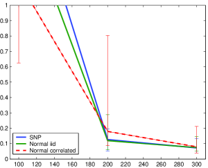
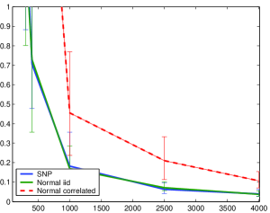
Figure 2 shows the decrease of the MSE as the sample size increases, when $M$ is kept fixed and set to $M=2000$ in this example. Figure 3 shows that for given configurations $(k^{*},2n)$ the size of the MSE is essentially unaffected by an increase in the number of predictors $M$ from 250 to 2000.

Figure 3. The median error vs number $M$ of predictors. Left: $2n=300,k^{*}=3$, right: $2n=1000,k^{*}=10$.

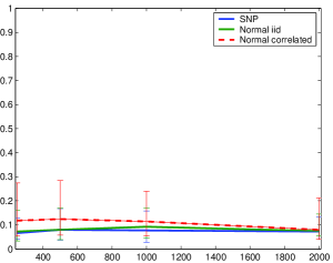
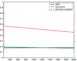
Our findings are consistent with the behavior of the Lasso estimates in other generalized linear models and with our Theorem 3.4 of Section 3. The overall conclusion is that the size of the MSE is influenced by the model size $k^{*}$ and not by $M$, the total number of variables in the model. When the variables $X_{j}$ are correlated, the MSE values are higher for the larger value of $k^{*}=10$ and very similar to the MSE values obtained for the uncorrelated variables when $k^{*}=3$. This supports the fact that the dependency structure of the variables $X_{j}$’s per se does not have a dramatic impact on the MSE, as suggested by our theoretical results of Section 3, which hold under the very mild Condition H on the design variables.

6.3. Variable selection accuracy

In this section we consider the same simulation scenario as above, and we shift focus to the quality of variable selection. In Figure 4 below we investigated the sensitivity of the estimated probability of correct variable selection, $I^{*}=\hat{I}$, or correct inclusion, $I^{*}\subseteq\hat{I}$, as we varied $M=250,500,1000,2000$. In the interest of space, we only report below the cases $k^{*}=3,2n=300$ (left column) and $k^{*}=10,2n=1000$ (right column).

Figure 4. The percentage of times $\hat{I}=I^{*}$(top row) and $I^{*}\subseteq\hat{I}$(bottom row) vs number $M$ of predictors. Left column: $k^{*}=3,2n=300$, right column: $k^{*}=10,2n=1000$.

Figure 5. The percentage of times $\hat{I}=I^{*}$(top row) and $I^{*}\subseteq\hat{I}$(bottom row) vs. number $2n$ of observations; $M=2000$. Left column: $k^{*}=3$, right column: $k^{*}=10$.

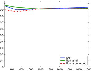
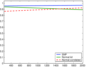
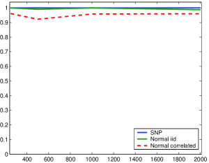
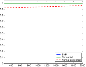
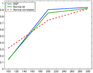
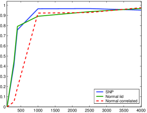
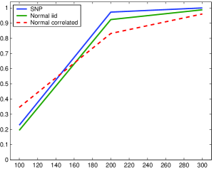
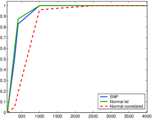
We present, in Figure 5 below, graphs of the percentage of times $I^{*}=\hat{I}$ and, respectively, $I^{*}\subseteq\hat{I}$, for $M=2000$, as we varied $n$, for $k^{*}=3$ and $k^{*}=10$. For ease of reference, we summarized in Table 2 the sample sizes needed to identify the true model at least 90% of the time.

	SNP	NOR_IID	NOR_CORR
$k^{*}=3$	200	250	300
$k^{*}=10$	800	1000	1000

Table 2. Sample sizes needed for $\mathbb{P}(\widehat{I}=I^{*})\geq 0.90$; M = 2000.

The results of this section support strongly the theoretical results of Section 4. Our method can identify the correct model with high probability. The accuracy of selection is influenced by the true model size $k^{*}$ and the dependence structure of the variables $X_{j}$, as shown in Figure 5 and it is much less influenced by an increase in the total number of the variables in the model, as shown in Figure 4.

7. Conclusions

We summarize our overall contributions in this section.

1. In this article we offered a theoretical analysis of the quality of model selection-type estimators in case-control studies. Our focus has been on optimizers of the $\ell_{1}$ regularized logistic likelihood. We showed that these estimators, analyzed under the case-control sampling scheme have model selection properties that are similar to those of the estimates analyzed under the prospective sampling scheme. In particular, we established the after model selection consistency of the odds ratio, and the consistency of subset selection. To the best of our knowledge, this is the first such theoretical analysis conducted for this sampling scheme.

2. We introduced a computationally efficient variable selection and dimension reduction procedure that uses a generalization of the Bisection Method, the GBM. We used the GBM to find simultaneously $M$ tuning parameters, each yielding an estimator with exactly $k$ non-zero entries, $1\leq k\leq M$. The final estimator is selected from the set of these $M$ candidates as the minimizer of a $p$-fold cross-validated log-likelihood to which we added a $BIC$-type penalty. This technique is general and can be used in connection with other loss functions and sparsity inducing penalty terms. The full theoretical investigation of this promising method is the subject of future research. All our simulation experiments indicate very good performance of this procedure in all the scenarios we considered. Moreover, our technique provides important computational savings over grid search based methods.

Appendix

Proof of Lemma 2.1. Let $(\widehat{\delta},\widehat{\beta})$ and $\widehat{q}$ be given by (2.1). We show that the maximum value of $\log L_{retros}(\delta,\beta,q)+pen(\beta)$, over all $({\delta},{\beta},{q})$ that satisfy the constraint (1.4), is bounded above and below by $\log L_{retros}(\widehat{\delta},\widehat{\beta},\widehat{q})+pen(\widehat{\beta})$. The bound from above is immediate, as a constraint maximum is always smaller or equal than the unconstrained maximum. To show the bound from below, we only need to verify that $(\widehat{\delta},\widehat{\beta},\widehat{q})$ given by (2.1) satisfy the constraint (1.4).

Let $G(\delta,\beta)=\log L_{pros}(\delta,\beta)+pen(\beta)$. If $(\widehat{\delta},\widehat{\beta})$ are given by (2.1), and $pen({\beta})$ is not a function of $\delta$ then, in particular, we have :

$$0=\frac{\partial\log G(\widehat{\delta},\widehat{\beta})}{\partial\delta}=\frac{\partial\log L_{pros}(\widehat{\delta},\widehat{\beta})}{\partial\delta}=n-\sum_{i=1}^{n}\widehat{p}_{1}(x^{0}_{i})-\sum_{i=1}^{n}\widehat{p}_{1}(x^{1}_{i}),$$

and also

$$n=\sum_{i=1}^{n}\widehat{p}_{0}(x^{0}_{i})+\sum_{i=1}^{n}\widehat{p}_{0}(x^{1}_{i}),$$

where $\widehat{p}_{j}$ denotes $p_{j}$ evaluated at $(\widehat{\delta},\widehat{\beta})$. Recall that the maximum likelihood estimator of $q$ is

$$\widehat{q}(x)=\frac{1}{2n}\left(\sum_{i=1}^{n}\delta_{x_{i}^{0}}(x)+\sum_{i=1}^{n}\delta_{x_{i}^{1}}(x)\right),$$

where $\delta_{a}$ denotes the Dirac function. Then, condition (1.4) is satisfied by $(\widehat{\delta},\widehat{\beta}),\widehat{q}$, since

$$\int\widehat{p}_{j}(x)\widehat{q}(x)dx=\frac{1}{2n}\left(\sum_{i=1}^{n}\widehat{p}_{j}(x^{0}_{i})+\sum_{i=1}^{n}\widehat{p}_{j}(x^{1}_{i})\right)=\frac{1}{2}.$$

This concludes the proof of this Lemma. $\blacksquare$

Proof of Theorem 3.1. We begin by introducing the notation used in the sequel. Let $\mathbb{P}_{n}^{0}=:\frac{1}{n}\sum_{i=1}^{n}\delta_{{X}_{i}^{0}}$ and $\mathbb{P}_{n}^{1}=:\frac{1}{n}\sum_{i=1}^{n}\delta_{{X}_{i}^{1}}$ denote the empirical measures associated with the two samples. For any function $g$ of generic argument $x$ we will use the notation $\mathbb{P}_{n}^{j}g(x)=\frac{1}{n}\sum_{i=1}^{n}g({x}_{i})$, for $j=0,1$. Recall that we defined the functions

$$\ell_{0}(\theta) =: \ell_{0}(\theta;x)\ =\ \log(1+e^{\theta^{\prime}x}),$$

$$\ell_{1}(\theta) =: \ell_{1}(\theta;x)\ =\ \log(1+e^{\theta^{\prime}x})-\theta^{\prime}x,$$

and recall the notation $\theta=(\delta,\beta)$. Then, by the definition of the estimator we have

$$\frac{1}{2}\left(\mathbb{P}_{n}^{0}\ell_{0}(\widehat{\theta})+\mathbb{P}_{n}^{1}\ell_{1}(\widehat{\theta})\right)+2r\sum_{j=1}^{M}|\widehat{\beta}_{j}| \leq \frac{1}{2}\left(\mathbb{P}_{n}^{0}\ell_{0}(\theta)+\mathbb{P}_{n}^{1}\ell_{1}(\theta)\right)$$

$$\ \ \ \ \ \ +\ 2r\sum_{j=1}^{M}|{\beta}_{j}|,$$

for all $\theta=(\delta,\beta)$. In particular, for $\theta=0$, this shows that

$$\sum_{j=1}^{M}|\widehat{\beta}_{j}|\leq\frac{\log 2}{2r}\ \ \ \ \ \ \mbox{and}\ \ \ \ \ \ |\widehat{\delta}|\leq\frac{L\log 2}{2r},$$

where $L$ is a common bound on $X_{ij}^{0},X_{ij}^{1}$ for all $i$ and $j$. Therefore, the estimator is effectively computed on the parameter set

(7.2) $$\mathcal{C}=\left\{\beta\in\mathbb{R}^{M},\delta\in\mathbb{R}:\ \ \sum_{j=1}^{M}|{\beta}_{j}|\leq\frac{\log 2}{2r},\ |{\delta}|\leq\frac{L\log 2}{2r}\right\},$$

and it is therefore enough to restrict our study to this set.

Recall that we defined $\Delta(\widehat{\theta},\theta^{*})$ in (3.2) as

$$\Delta(\widehat{\theta},\theta^{*})=\frac{1}{2}\mathbb{P}^{0}\left(\ell_{0}(\widehat{\theta})-\ell_{0}(\theta^{*})\right)+\frac{1}{2}\mathbb{P}^{1}\left(\ell_{1}(\widehat{\theta})-\ell_{1}(\theta^{*})\right).$$

Note further that since (Appendix) holds for all $\theta$ it holds in particular for for $\theta=\theta^{*}$. Then, by adding $\Delta(\widehat{\theta},\theta^{*})+r\sum_{j=1}^{M}|\widehat{\beta}_{j}-\beta_{j}^{*}|$ to both sides of (Appendix) and re-arranging terms we obtain

(7.3) $$r\sum_{j=1}^{M}|\widehat{\beta}_{j}-\beta_{j}^{*}|+\Delta(\widehat{\theta},\theta^{*})\leq\frac{1}{2}(\mathbb{P}_{n}^{0}-\mathbb{P}^{0})\left(\ell_{0}(\theta^{*})-\ell_{0}(\widehat{\theta})\right)$$

$$\hskip 128.0374pt+\ \frac{1}{2}(\mathbb{P}_{n}^{1}-\mathbb{P}^{1})\left(\ell_{1}(\theta^{*})-\ell_{1}(\widehat{\theta})\right)$$

$$\hskip 128.0374pt+\ r\sum_{j=1}^{M}|\widehat{\beta}_{j}-\beta_{j}^{*}|+2r\sum_{j=1}^{M}|\beta_{j}^{*}|-2r\sum_{j=1}^{M}|\widehat{\beta}_{j}|.$$

Let $\epsilon>0$ be a quantity that will be made precise below. Then, for $\theta\in\mathcal{C}$ given by (7.2) above we define

$$\mathcal{L}_{n}^{0} = \sup_{\theta\in\mathcal{C}}\frac{|(\mathbb{P}_{n}^{0}-\mathbb{P}^{0})(l_{0}(\theta^{*})-l_{0}({\theta}))|}{|\beta-\beta^{*}|_{1}+\frac{|\delta-\delta^{*}|}{\log n}+\epsilon},$$

$$\mathcal{L}_{n}^{1} = \sup_{\theta\in\mathcal{C}}\frac{|(\mathbb{P}_{n}^{1}-\mathbb{P}^{1})(l_{1}(\theta^{*})-l_{1}({\theta}))|}{|\beta-\beta^{*}|_{1}+\frac{|{\delta}-\delta^{*}|}{\log n}+\epsilon},$$

where $|v|_{1}=\sum_{j=1}^{d}|v_{j}|$ denotes the $\ell_{1}$ norm of a generic vector $v\in\mathbb{R}^{d}$, for some $d$. Define the events

(7.4) $$\mathcal{E}_{0}=\left\{\mathcal{L}_{n}^{0}\leq r\},\ \mathcal{E}_{1}=\{\mathcal{L}_{n}^{1}\leq r\right\}.$$

Then, on $\mathcal{E}_{0}\cap\mathcal{E}_{1}$ display (7.3) above yields

(7.5) $$r\sum_{j=1}^{M}|\widehat{\beta}_{j}-\beta_{j}^{*}|+\Delta(\widehat{\theta},\theta^{*})$$

$$\hskip 8.5359pt\leq\ 2r\sum_{j=1}^{M}|\widehat{\beta}_{j}-\beta_{j}^{*}|+2r\sum_{j=1}^{M}|\beta_{j}^{*}|-2r\sum_{j=1}^{M}|\widehat{\beta}_{j}|$$

$$\hskip 8.5359pt+\ r\frac{|\widehat{\delta}-\delta^{*}|}{\log n}+r\epsilon.$$

We will argue below that:

Fact 1. $\Delta(\widehat{\theta},\theta^{*})\geq 0$.

Fact 2. $\mathbb{P}(\mathcal{E}_{0}^{c})\rightarrow 0$ and $\mathbb{P}(\mathcal{E}_{1}^{c})\rightarrow 0$.

Assume that Fact 1 and Fact 2 hold. Then, if Fact 1 holds, both terms in the left hand side of display (7.5) are positive. Thus, in particular, display (7.5) yields on the event $\mathcal{E}_{0}\cap\mathcal{E}_{1}$ that

$$\Delta(\widehat{\theta},\theta^{*})\leq\ 2r\sum_{j=1}^{M}|\widehat{\beta}_{j}|+2r\sum_{j=1}^{M}|\beta_{j}^{*}|+2r\sum_{j=1}^{M}|\beta_{j}^{*}|-2r\sum_{j=1}^{M}|\widehat{\beta}_{j}|$$

$$\hskip 56.9055pt+\ r\frac{|\widehat{\delta}-\delta^{*}|}{\log n}+r\epsilon$$

$$\hskip 54.06006pt\leq 4r\sum_{j\in I^{*}}|\beta_{j}^{*}|+r\frac{|\widehat{\delta}-\delta^{*}|}{\log n}+r\epsilon.$$

Recall now that we have assumed that $\max_{j\in I^{*}}|\beta_{j}^{*}|\leq B,|\delta^{*}|\leq B$, for some positive constant $B$ and that $\widehat{\delta}\in\mathcal{C}$, and so $|\widehat{\delta}|\leq\frac{L\log 2}{2r}$. Thus, on the event $\mathcal{E}_{0}\cap\mathcal{E}_{1}$, we have

$$\Delta(\widehat{\theta},\theta^{*})\leq 4rk^{*}B+\frac{L\log 2}{2\log n}+r\frac{B}{\log n}+r\epsilon.$$

Then, for our choice of $r$, under the assumption that $rk^{*}\rightarrow 0$ and for the choice of $\epsilon$ given below in (7.11), the right hand side of the above display converges to zero with $n$. Therefore, for any $\alpha>0$ we have the desired result:

(7.6) $$\mathbb{P}(\Delta(\widehat{\theta},\theta^{*})>\alpha)\leq\mathbb{P}(\mathcal{E}_{0}^{c})+\mathbb{P}(\mathcal{E}_{1}^{c})\longrightarrow 0,$$

provided Fact 2 holds. We argue in what follows that the two facts hold.

Proof of Fact 1. Recall the definition (1.3) of $f_{0}(x)$, $f_{1}(x)$, $q(x)$ and $p_{1}(x)$, and notice that we have $f_{0}(x)+f_{1}(x)=2q(x)$. Let $\bar{\theta}^{\prime}x$ be an intermediate point between $\theta^{*\prime}x$ and $\widehat{\theta}^{\prime}x$. Then, a second order Taylor expansion gives:

$$\Delta(\widehat{\theta},\theta^{*}) = \int\left(\log(1+\exp(\widehat{\theta}^{\prime}x))-\log(1+\exp({\theta}^{*\prime}x))\right)q(x)dx$$

$$-\int(\widehat{\theta}^{\prime}x-{\theta}^{*\prime}x)p_{1}(x)q(x)dx$$

$$= \int(\widehat{\theta}^{\prime}x-{\theta}^{*\prime}x)p_{1}(x)q(x)dx$$

$$+\ \frac{1}{2}\int\frac{\exp(\bar{\theta}^{\prime}x)}{(1+\exp(\bar{\theta}^{\prime}x))^{2}}(\widehat{\theta}^{\prime}x-{\theta}^{*\prime}x)^{2}q(x)dx$$

$$-\int(\widehat{\theta}^{\prime}x-{\theta}^{*\prime}x)p_{1}(x)q(x)dx$$

$$= \frac{1}{4}\int\frac{\exp(\bar{\theta}^{\prime}x)}{(1+\exp(\bar{\theta}^{\prime}x))^{2}}(\widehat{\theta}^{\prime}x-{\theta}^{*\prime}x)^{2}f_{0}(x)dx$$

$$+\ \frac{1}{4}\int\frac{\exp(\bar{\theta}^{\prime}x)}{(1+\exp(\bar{\theta}^{\prime}x))^{2}}(\widehat{\theta}^{\prime}x-{\theta}^{*\prime}x)^{2}f_{1}(x)dx,$$

which shows that the left hand side is positive.

Proof of Fact 2. Define the re-scaled empirical processes

$$\mathbb{G}_{n}^{0}=\sup_{\theta\in\mathcal{C}}\frac{|(\mathbb{P}_{n}^{0}-\mathbb{P}^{0})(l_{0}(\theta^{*})-l_{0}({\theta}))|}{|\beta-\beta^{*}|_{1}+|\delta-\delta^{*}|+\epsilon}\ \ \mbox{and},$$

$$\mathbb{G}_{n}^{1}=\sup_{\theta\in\mathcal{C}}\frac{|(\mathbb{P}_{n}^{1}-\mathbb{P}^{1})(l_{1}(\theta^{*})-l_{1}({\theta}))|}{|\beta-\beta^{*}|_{1}+|{\delta}-\delta^{*}|+\epsilon},$$

and notice that

(7.8) $$\mathbb{P}(\mathcal{E}_{0}^{c})\leq\mathbb{P}\left(\mathbb{G}_{n}^{0}>\frac{r}{\log n}\right)\ \ \ \mbox{and}\ \ \ \mathbb{P}(\mathcal{E}_{1}^{c})\leq\mathbb{P}\left(\mathbb{G}_{n}^{1}>\frac{r}{\log n}\right).$$

The proof of Fact 2 therefore relies on the control of $\mathbb{G}_{n}^{0}$ and $\mathbb{G}_{n}^{1}$. For this, we use the bounded difference inequality, see e.g. Theorem 2.2, page 8 in [9]. To apply it we need to evaluate by how much ${\mathbb{G}}_{n}^{0}$ and ${\mathbb{G}}_{n}^{1}$ change if we change the $i$-th variable $X_{i}^{0}$, $X_{i}^{1}$, respectively, while keeping the others fixed. Recall that $\mathbb{P}_{n}^{0}=\frac{1}{n}\sum_{i=1}^{n}\delta_{X_{i}^{0}}$ is the empirical measure putting mass $1/n$ at each observation $X_{i}$. Let $\mathbb{P}^{0\prime}_{n}$ be the empirical measure $\frac{1}{n}\left(\sum_{i=1,i\neq l}^{n-1}\delta_{X_{i}^{0}}+\delta_{X_{l}^{0\prime}}\right)$ corresponding to changing the pair $X_{l}^{0}$ to $X_{l}^{0\prime}$. Then

$$\frac{(\mathbb{P}_{n}^{0}-\mathbb{P}^{0})(l_{0}(\theta^{*})-l_{0}({\theta}))}{|\beta-\beta^{*}|_{1}+|\delta-\delta^{*}|+\epsilon}-\frac{(\mathbb{P}^{0\prime}_{n}-\mathbb{P}^{0})(l_{0}(\theta^{*})-l_{0}({\theta}))}{|\beta-\beta^{*}|_{1}+|\delta-\delta^{*}|+\epsilon}$$

$$\hskip 5.69046pt=\frac{1}{n}\frac{l_{0}(\theta^{*};X_{l}^{0})-l_{0}({\theta};X_{l}^{0})-l_{0}(\theta^{*};X_{l}^{0\prime})+l_{0}({\theta};X_{l}^{0\prime})}{|\beta-\beta^{*}|_{1}+|\delta-\delta^{*}|+\epsilon}$$

(7.9) $$\hskip 5.69046pt\leq\frac{4L}{n}\frac{|\beta-\beta^{*}|_{1}+|\delta-\delta^{*}|}{|\beta-\beta^{*}|_{1}+|\delta-\delta^{*}|+\epsilon}\leq\frac{4L}{n},$$

where the inequality follows immediately by a first order Taylor expansion and the assumption that all $X$ variables are bounded by $L>1$. The calculations involving ${\mathbb{G}}^{1}_{n}$ are identical, and yield the bound $\frac{8L}{n}$. Therefore, we can apply the bounded difference inequality to obtain that

(7.10) $$\mathbb{P}^{0}({\mathbb{G}}_{n}^{0}-\mathbb{E}^{0}{\mathbb{G}}^{0}_{n}\geq u) \leq \exp{-\frac{nu^{2}}{8L^{2}}},$$

$$\mathbb{P}^{1}({\mathbb{G}}_{n}^{1}-\mathbb{E}^{1}{\mathbb{G}}^{1}_{n}\geq u) \leq \exp{-\frac{nu^{2}}{32L^{2}}}.$$

We will use Lemma 3 in [27] to obtain bounds on $\mathbb{E}^{0}\mathbb{G}_{n}^{0}$ and $\mathbb{E}^{1}\mathbb{G}_{n}^{1}$. We re-state a version of it here, for ease of reference.

Let $J_{n}$ be an integer such that $2^{J_{n}}\geq n$ and $0<\epsilon\leq\frac{\log 2}{r}$ Then, if the functions $l_{0}$ and $l_{1}$ defined above are Lipschitz in $\theta^{\prime}x$ and the components of $x$ are bounded by $L$, with probability one, then both $\mathbb{E}^{0}\mathbb{G}_{n}^{0},\ \mathbb{E}^{1}\mathbb{G}_{n}^{1}$ are bounded by $C_{1}\sqrt{\frac{2\log 2(M\vee n)}{n}}+C_{2}\frac{J_{n}}{2(M\vee n)^{2}}$, where $C_{1},C_{2}$ are positive constants depending on the respective Lipschitz constants and $L$.

Notice that $l_{0}$ and $l_{1}$ are Lipschitz in $t=\theta^{\prime}x$, with respective constants 1 and 2. Also, inspection of the chaining argument used in the proof of this lemma shows that we can take $J_{n}=(M\vee n)$ and

(7.11) $$\epsilon=\frac{\log 2}{2^{(M\vee n)+1}}\times\frac{1}{r},$$

for $r$ given in (3.3), which we also recall here

$$r=\log n\left(6L\sqrt{\frac{2\log 2(M\vee n)}{n}}+\frac{1}{4(M\vee n)}+4L\sqrt{\frac{2\log\frac{1}{\delta}}{n}}\right).$$

Then, making the constants precise in the lemma above and taking

(7.12) $$u=4L\sqrt{\frac{2\log\frac{1}{\delta}}{n}},$$

display (7.10) yields

$$\mathbb{P}^{0}\left({\mathbb{G}}_{n}^{0}\geq\frac{r}{\log n}\right)\leq\delta,\ \ \mathbb{P}^{1}\left({\mathbb{G}}_{n}^{1}\geq\frac{r}{\log n}\right)\leq\delta,$$

for any $\delta>0$, in particular for any $\delta=\delta_{n}\rightarrow 0$. This display in combination with (7.8) above gives the desired result. This completes the proof of this theorem.  $\blacksquare$

Proof of Corollary 3.2. By definition

$$\Delta(\widehat{\theta},\theta^{*}) = \int\left(\log(1+\exp(\widehat{\theta}^{\prime}x))-\log(1+\exp({\theta}^{*\prime}x))\right)q(x)dx$$

$$-\int(\widehat{\theta}^{\prime}x-{\theta}^{*\prime}x)p_{1}(x)q(x)dx$$

$$= \int(\widehat{\theta}^{\prime}x-{\theta}^{*\prime}x)\left(\frac{\exp(\bar{\theta}^{\prime}x)}{1+\exp(\bar{\theta}^{\prime}x)}-\frac{\exp({\theta}^{*\prime}x)}{1+\exp({\theta}^{*\prime}x)}\right)q(x)dx,$$

where the last line follows via a first order Taylor expansion. Simple algebraic manipulations show that if $\sup_{x}|\widehat{\theta}^{\prime}{x}-{\theta}^{*\prime}{x}|\geq\gamma$, for any $\gamma>0$, then $\Delta(\widehat{\theta},\theta^{*})>0$. Therefore, there exits $\alpha_{\gamma}$ such that $\Delta(\widehat{\theta},\theta^{*})\geq\alpha_{\gamma}$. Invoking Theorem 3.1 above we therefore obtain

(7.13) $$\mathbb{P}\left(\sup_{x}|\widehat{\theta}^{\prime}{x}-{\theta}^{*\prime}{x}|\geq\gamma\right)\leq\mathbb{P}\left(\Delta(\widehat{\theta},\theta^{*})>\alpha_{\gamma}\right)\longrightarrow 0,$$

which is the desired result. $\blacksquare$

Proof of Theorem 3.3. Recall that in (Appendix) above we showed that

$$\Delta(\widehat{\theta},\theta^{*}) = \frac{1}{4}\int\frac{\exp(\bar{\theta}^{\prime}x)}{(1+\exp(\bar{\theta}^{\prime}x))^{2}}(\widehat{\theta}^{\prime}x-{\theta}^{*\prime}x)^{2}f_{0}(x)dx$$

$$+\ \frac{1}{4}\int\frac{\exp(\bar{\theta}^{\prime}x)}{(1+\exp(\bar{\theta}^{\prime}x))^{2}}(\widehat{\theta}^{\prime}x-{\theta}^{*\prime}x)^{2}f_{1}(x)dx,$$

with $\bar{\theta}^{\prime}x$ being an intermediate point between $\theta^{*\prime}x$ and $\widehat{\theta}^{\prime}x$.

Let $\gamma>0$ be arbitrarily close to zero, fixed. Let $A_{\gamma}=\{\sup_{x}|\widehat{\theta}^{\prime}{x}-{\theta}^{*\prime}{x}|\leq\gamma\}$. By (7.13) above we have $\mathbb{P}(A_{\gamma})\rightarrow 1$. On $A_{\gamma}$ we have ${\theta}^{*\prime}{x}\geq\bar{\theta}^{\prime}x-\gamma$, for all $x$, and therefore

$$\frac{\exp(\bar{\theta}^{\prime}x)}{(1+\exp(\bar{\theta}^{\prime}x))^{2}} = \exp(\bar{\theta}^{\prime}x-{\theta}^{*\prime}x)\left(\frac{1+\exp({\theta}^{*\prime}x)}{1+\exp(\bar{\theta}^{\prime}x)}\right)^{2}p_{0}(x)p_{1}(x)$$

$$\geq \frac{\exp(\bar{\theta}^{\prime}x-{\theta}^{*\prime}x)}{\exp(2\gamma)}$$

$$\geq \exp(-3\gamma)p_{0}(x)p_{1}(x)=:wp_{0}(x)p_{1}(x),$$

for all $x$ and with $w$ arbitrarily close to one. Recall that $f(x)=\pi f_{0}(x)+(1-\pi)f_{1}(x)$, for $\mathbb{P}(Y=1)=\pi$. Then, on the set $A_{\gamma}$ we have

$$\Delta(\widehat{\theta},\theta^{*}) \geq \frac{w}{4}\int p_{0}(x)p_{1}(x)(\widehat{\theta}^{\prime}x-{\theta}^{*\prime}x)^{2}(f_{1}(x)+f_{0}(x))dx,$$

$$\geq \frac{w}{4}\int p_{0}(x)p_{1}(x)(\widehat{\theta}^{\prime}x-{\theta}^{*\prime}x)^{2}f(x)dx$$

$$\geq wb\left(\sum_{j\in I^{*}}(\widehat{\beta}_{j}-\beta_{j}^{*})^{2}+(\widehat{\delta}-\delta^{*})^{2}\right),$$

where the last inequality follows from Condition H. Then, adding and subtracting $r|\widehat{\delta}-\delta^{*}|$ to both sides in (7.5) and using (Appendix) above we obtain

$$r|\widehat{\delta}-\delta^{*}|+r\sum_{j=1}^{M}|\widehat{\beta}_{j}-\beta_{j}^{*}|+wb\sum_{j\in I^{*}}(\widehat{\beta}_{j}-\beta_{j}^{*})^{2}+wb(\widehat{\delta}-\delta^{*})^{2}$$

$$\leq\ 2r\sum_{j=1}^{M}|\widehat{\beta}_{j}-\beta_{j}^{*}|+2r\sum_{j=1}^{M}|\beta_{j}^{*}|-2r\sum_{j=1}^{M}|\widehat{\beta}_{j}|+r(1+\frac{1}{\log n})|\widehat{\delta}-\delta^{*}|+r\epsilon$$

$$\leq 4r\sum_{j\in I^{*}}|\widehat{\beta}_{j}-\beta_{j}^{*}|+r(1+\frac{1}{\log n})|\widehat{\delta}-\delta^{*}|+r\epsilon$$

$$\leq\frac{6}{bw}r^{2}k^{*}+wb\sum_{j\in I^{*}}(\widehat{\beta}_{j}-\beta_{j}^{*})^{2}+wb(\widehat{\delta}-\delta^{*})^{2},$$

where we obtained the last line by using the Cauchy-Schwarz inequality followed by an inequality of the type $2uv\leq au^{2}+v^{2}/a$, for any $a>1$. For clarity of exposition, we absorbed the term $r\epsilon$, which is of order $1/2^{M\vee n}$, into the first term, which is much larger. Therefore

$$r|\widehat{\delta}-\delta^{*}|+r\sum_{j=1}^{M}|\widehat{\beta}_{j}-\beta_{j}^{*}|\leq\frac{6}{bw}r^{2}k^{*},$$

which implies

$$|\widehat{\delta}-\delta^{*}| \leq \frac{6}{bw}rk^{*},$$

$$\sum_{j=1}^{M}|\widehat{\beta}_{j}-\beta_{j}^{*}| \leq \frac{6}{bw}rk^{*},$$

on the set $A_{\gamma}$, with $\mathbb{P}(A_{\gamma})\rightarrow 1$, which is the desired result. $\blacksquare$

Proof of Theorem 4.1. Since $\mathbb{P}(I^{*}=\hat{I})\geq 1-\mathbb{P}(I^{*}\not\subseteq\hat{I})-\mathbb{P}(\widehat{I}\not\subseteq I^{*})$, it is enough to control the two probabilities in the right hand side of this inequality separately.

Control of $\mathbb{P}(I^{*}\not\subseteq\hat{I})$.

Recall that we denoted the cardinality of $I^{*}$ by $k^{*}$. Then, by the definition of the sets $\widehat{I}$ and $I^{*}$ we have

$$\mathbb{P}(I^{*}\not\subseteq\hat{I}) \leq \mathbb{P}\left(k\notin\hat{I}\ {\mbox{f}or\ some}\ k\in I^{*}\right)$$

$$\leq k^{*}\max_{k\in I^{*}}\ \mathbb{P}\left(\widehat{\beta}_{k}=0\ \mbox{and}\ \beta^{*}_{k}\neq 0\right)$$

$$\leq M\max_{k\in I^{*}}\ \mathbb{P}\left(\widehat{\beta}_{k}=0\ \mbox{and}\ \beta^{*}_{k}\neq 0\right),$$

as we always have $k^{*}\leq M$. Recall that

$$\log L_{pros}(\theta)\\ =\sum_{i=1}^{n}\log(1+e^{\theta^{\prime}{X}_{i}^{0}})-\sum_{i=1}^{n}(\theta^{\prime}{X}_{i}^{1})+\sum_{i=1}^{n}\log(1+e^{\theta^{\prime}{X}_{i}^{1}}),$$

and let $L_{n}(\theta)=\log L_{pros}(\theta)$. By standard results in convex analysis, if $\widehat{\beta}_{k}=0$ is a component of the solution $\widehat{\theta}=(\widehat{\delta},\widehat{\beta})$ then

$$\left|\frac{\partial L_{n}(\widehat{\theta})}{\partial\beta_{k}}\right|<2r.$$

Let $k$ be arbitray, fixed. Define

(7.15) $$T_{n}(\widehat{\theta})=:T_{n} = \frac{\partial L_{n}(\widehat{\theta})}{\partial\beta_{k}}-\frac{\partial L_{n}({\theta^{*}})}{\partial\beta_{k}}$$

$$S_{n}(\widehat{\theta})=:S_{n} = \sum_{j=0}^{M}(\widehat{\theta}_{j}-\theta_{j}^{*})\left(\frac{1}{2n}\sum_{i=1}^{2n}X_{ij}X_{ik}\right).$$

Recall that by convention $X_{i0}=1$, for all $i$, and for compactness of notation we will write $\widehat{\theta}_{0}=\widehat{\delta}$ and $\theta_{0}^{*}=\delta$.

Assuming without loss of generality that the data has been scaled such that $\frac{1}{2n}\sum_{i=1}^{n}X_{ik}^{2}=1$ for all $k$, we therefore obtain, for every $k\in I^{*}$, that

$$\mathbb{P}\left(\widehat{\beta}_{k}=0\ \mbox{and}\ \beta^{*}_{k}\neq 0\right)$$

$$\quad\leq\mathbb{P}\left(\left|T_{n}-S_{n}+S_{n}+\frac{\partial L_{n}({\theta^{*}})}{\partial\beta_{k}}\right|\leq 2r;\ \ \beta_{k}^{*}\neq 0\right)$$

$$\quad\leq\mathbb{P}\left(|S_{n}|-|S_{n}-T_{n}|-\left|\frac{\partial L_{n}({\theta^{*}})}{\partial\beta_{k}}\right|\leq 2r;\ \ \ \beta_{k}^{*}\neq 0\right)$$

$$\quad\leq\mathbb{P}\left(|\beta_{k}^{*}|\,{-}\,\Bigg{|}\sum_{j\neq k}(\widehat{\theta}_{j}\,{-}\,\theta_{j}^{*})\frac{1}{2n}\sum_{i=1}^{2n}X_{ij}X_{ik}\Bigg{|}\,{-}\,|S_{n}-T_{n}|\,{-}\,\left|\frac{\partial L_{n}({\theta^{*}})}{\partial\beta_{k}}\right|\leq 2r\right).$$

Therefore

(7.16) $$\mathbb{P}(I^{*}\not\subseteq\hat{I})\leq M\max_{k\in I^{*}}\ \mathbb{P}\left(\left|\frac{\partial L_{n}({\theta^{*}})}{\partial\beta_{k}}\right|\geq\frac{|\beta_{k}^{*}|-2r}{3}\right)$$

$$\hskip 56.9055pt+\ M\max_{k\in I^{*}}\mathbb{P}\left(\sum_{j=0}^{M}|\widehat{\theta}_{j}-\theta_{j}^{*}|\Bigg{|}\frac{1}{2n}\sum_{i=1}^{2n}X_{ij}X_{ik}\Bigg{|}>\frac{|\beta_{k}^{*}|-2r}{3}\right)$$

$$\hskip 56.9055pt+\ M\max_{k\in I^{*}}\mathbb{P}\left(|S_{n}-T_{n}|\geq\frac{|\beta_{k}^{*}|-2r}{3}\right)$$

$$\hskip 51.21504pt=(I)+(II)+(III).$$

In what follows we bound each of the above terms individually.

Bound on (III). Let $\bar{\theta}^{\prime}{X}_{i}$ be a point between $\widehat{\theta}^{\prime}{X}_{i}$ and ${\theta}^{*\prime}{X}_{i}$, for each $i$. A first order Taylor expansion yields

$$T_{n} = \frac{1}{2n}\sum_{j=0}^{M}\sum_{i=1}^{2n}X_{ij}X_{ik}\frac{\exp(\bar{\theta}^{\prime}{X}_{i})}{(1+\exp(\bar{\theta}^{\prime}{X}_{i}))^{2}}(\widehat{\theta}_{j}\,{-}\,\theta_{j}^{*})$$

$$= \frac{1}{2n}\sum_{j=0}^{M}\sum_{i=1}^{2n}X_{ij}X_{ik}\frac{\exp(\bar{\theta}^{\prime}{X}_{i}-\theta^{*\prime}X_{i})}{(1+\exp(\bar{\theta}^{\prime}{X}_{i}-\theta^{*\prime}X_{i}))^{2}}p_{1}(X_{i})p_{0}(X_{i})(\widehat{\theta}_{j}\,{-}\,\theta_{j}^{*}),$$

where the last line follows from the first by dividing and multiplying the summands by $p_{1}(X_{i})p_{0}(X_{i})$ defined in (1.3) above. Let $\gamma$ be arbitrarily close to zero, fixed. Let $D_{\gamma}$ be the set on which $\sup_{x}|\widehat{\theta}^{\prime}x-\theta^{*\prime}x|\leq\gamma$. Corollary 3.2 above guarantees that $\mathbb{P}(D_{\gamma}^{c})\rightarrow 0$. Since $\gamma$ is arbitrarily close to zero, the difference

$$|D_{ni}|=:\left|\frac{\exp(\bar{\theta}^{\prime}{X}_{i}-\theta^{*\prime}X_{i})}{(1+\exp(\bar{\theta}^{\prime}{X}_{i}-\theta^{*\prime}X_{i}))^{2}}-\frac{1}{4}\right|\leq\vartheta,$$

with $\vartheta$ arbitrarily close to 0, for each $i$, on the set $D_{\gamma}$. Therefore we have

$$\mathbb{P}\left(|S_{n}-T_{n}|\geq\frac{|\beta_{k}^{*}|-2r}{3}\right)$$

$$\leq\mathbb{P}\left(\left|\frac{1}{2n}\sum_{j=0}^{M}\sum_{i=1}^{2n}X_{ij}X_{ik}\left(1-\frac{p_{1}(X_{i})p_{0}(X_{i})}{4}\right)(\widehat{\theta}_{j}\,{-}\,\theta_{j}^{*})\right|\geq\frac{|\beta_{k}^{*}|-2r}{6}\right)$$

$$\ \ +\ \mathbb{P}\left(\left|\frac{1}{2n}\sum_{j=0}^{M}\sum_{i=1}^{2n}D_{ni}X_{ij}X_{ik}(\widehat{\theta}_{j}\,{-}\,\theta_{j}^{*})\right|\geq\frac{|\beta_{k}^{*}|-2r}{6}\right)+\mathbb{P}(D_{\gamma}^{c})$$

$$=:(a)+(b)+\mathbb{P}(D_{\gamma}^{c}).$$

To bound $(a)$ we first invoke Conditions 1 and 2 to obtain that

$$\left|\frac{1}{2n}\sum_{j=0}^{M}\sum_{i=1}^{2n}X_{ij}X_{ik}\left(1-\frac{p_{1}(X_{i})p_{0}(X_{i})}{4}\right)(\widehat{\theta}_{j}\,{-}\,\theta_{j}^{*})\right|\leq\frac{C}{k^{*}}\sum_{j=0}^{M}|\widehat{\theta}_{j}\,{-}\,\theta_{j}^{*}|,$$

where $C$ is a positive constant, independent of $n$ and depending only on the constant $d$ of Conditions 1 and 2. Combining this with the assumption that $\min_{k\in I^{*}}|\beta_{k}^{*}|>4r$ we arrive at

$$(a)\leq\mathbb{P}\left(\sum_{j=0}^{M}|\widehat{\theta}_{j}\,{-}\,\theta_{j}^{*}|\geq ck^{*}r\right),$$

for some positive constant $c$ depending only on $d$ and not on $n$.

To bound $(b)$ we recall that all $X$ variables are bounded by $L$ and that $|D_{ni}|$ is bounded by $\vartheta$. Note that we can always choose $\vartheta=\frac{1}{k^{*}}$, as we can always choose the corresponding $\gamma$. Therefore, the resulting bound is

$$(b)\leq\mathbb{P}\left(\sum_{j=0}^{M}|\widehat{\theta}_{j}\,{-}\,\theta_{j}^{*}|\geq c_{1}k^{*}r\right),$$

for some $c_{1}>0$ depending on $L$ and not on $n$. Collecting the bounds above we thus have

$$(III)\leq M\mathbb{P}\left(\sum_{j=0}^{M}|\widehat{\theta}_{j}\,{-}\,\theta_{j}^{*}|\geq ck^{*}r\right)+M\mathbb{P}\left(\sum_{j=0}^{M}|\widehat{\theta}_{j}\,{-}\,\theta_{j}^{*}|\geq c_{1}k^{*}r\right)$$

$$\hskip 31.2982pt\ \ \ +\ M\mathbb{P}(D_{\gamma}^{c})$$

$$\hskip 28.45274pt\leq 3M(\mathbb{P}(\mathcal{E}^{0})+\mathbb{P}(\mathcal{E}^{1})),$$

where the last line follows from the proofs of Theorem 3.3 and Corollary 3.2, for sets $\mathcal{E}^{0},\mathcal{E}^{1}$ defined as in (7.4) above, and with $r$ replaced by the slightly larger value given in (4.1) above. Then, as in the proof of Fact 2 of Theorem 3.1 and for this value of $r$, we obtain

$$(III)\ \leq 3M\frac{2\delta}{M}\leq 6\delta\longrightarrow 0,$$

for any $\delta=\delta_{n}\rightarrow 0$, as $n\rightarrow\infty$.

Bound on (II). We reason exactly as above, using now Assumption 2 and Condition 1 to obtain, for some constant $c>0$, that

(7.17) $$(II) \leq M\mathbb{P}\left(\sum_{j=0}^{M}|\widehat{\theta}_{j}\,{-}\,\theta_{j}^{*}|\geq ck^{*}r\right)$$

$$\leq M(\mathbb{P}(\mathcal{E}^{0})+\mathbb{P}(\mathcal{E}^{1}))\leq M\frac{2\delta}{M}\leq 2\delta\longrightarrow 0,$$

for any $\delta=\delta_{n}\rightarrow 0$, as $n\rightarrow\infty$.

Bound on (I). First notice that, for any $k$ we have

$$\frac{\partial L_{n}({\theta^{*}})}{\partial\beta_{k}}=\frac{1}{2n}\left\{\sum_{i=1}^{n}X_{ik}^{0}p_{1}(X_{i}^{0})-\sum_{i=1}^{n}{X}_{ik}^{1}+\sum_{i=1}^{n}X_{ik}^{1}p_{1}(X_{i}^{1})\right\}.$$

Let

$$Z_{ik}=X_{ik}^{0}p_{1}(X_{i}^{0})+X_{ik}^{1}p_{1}(X_{i}^{1})-{X}_{ik}^{1},$$

and notice that $\mathbb{E}Z_{ik}=0$, for all $i$ and $k$. Since $|Z_{ik}|\leq 3L$, we use Hoeffding’s inequality to obtain

$$\mathbb{P}\left(\left|\frac{\partial L_{n}({\theta^{*}})}{\partial\beta_{k}}\right|\geq v\right)\leq\exp\left(-\frac{2nv^{2}}{9L^{2}}\right),$$

and this is bounded by $\delta/M$ for any $v\geq\frac{3L\sqrt{\log M/\delta}}{\sqrt{2n}}$. Thus, by Assumption 2 and our choice of $r$ given in (4.1), we have that $(I)\leq\delta.$

Collecting now the bounds on $(I),(II)$ and $(III)$ we therefore obtain

$$\mathbb{P}(I^{*}\not\subseteq\hat{I})\leq 9\delta\rightarrow 0,$$

for any $\delta=\delta_{n}\rightarrow 0$, as $n\rightarrow\infty$, which completes the first part of the proof.

Control of $\mathbb{P}(\widehat{I}\not\subseteq I^{*})$. The control of this quantity will essentially involve the usage of the same probability bounds as above. We will however need a different intermediate argument. Let $\mu\in\mathbb{R}^{k^{*}+1}$, where we denote the first component of $\mu$ by $\delta$. Define

$$H(\mu) = \frac{1}{2n}\left\{\sum_{i=1}^{2n}\log(1+e^{\mu^{\prime}X_{i}^{0}})-\sum_{i=1}^{n}(\mu^{\prime}X_{i}^{1})+\sum_{i=1}^{n}\log(1+e^{\mu^{\prime}X_{i}^{1}})\right\}$$

$$\ +\ 2r\sum_{j\in I^{*}}|\mu_{j}|,$$

and define

(7.18) $$\widetilde{\mu}=\mathop{\arg\min}_{\mu\in\mathbb{R}^{k^{*}+1}}H(\mu),$$

where by convention we denote the first component of $\widetilde{\mu}$ by $\widetilde{\delta}$. Let, by abuse of notation, $\widetilde{\mu}\in\mathbb{R}^{M+1}$ be the vector that has the first component $\widetilde{\delta}$, the other components of $\widetilde{\mu}$ in positions corresponding to the index set $I^{*}$, and is zero otherwise. Define the set

$$\mathcal{B}_{1}=\bigcap_{k\notin I^{*}}\left\{\left|\frac{\partial L_{n}(\widetilde{\mu})}{\partial\beta_{k}}\right|<2r\right\}.$$

By standard results in convex analysis it follows that, on the set $\mathcal{B}_{1}$, $\widetilde{\mu}$ is a solution of (2). Recall that $\widehat{\theta}$ is a solution of (2) by construction. Then, using simple convex analysis arguments as in Proposition 4.2 in Bunea (2008), we obtain that any two solutions have non-zero elements in the same positions. Since, on the set $\mathcal{B}_{1}$, $\widehat{\theta}_{k}=0$ for $k\in{I^{*}}^{c}$ we conclude that $\hat{I}\subseteq I^{*}$ on the set $\mathcal{B}_{1}$. Hence

(7.19) $$\mathbb{P}(\hat{I}\not\subseteq I^{*})\ \leq\ \mathbb{P}(\mathcal{B}_{1}^{c})$$

$$\hskip 48.36958pt\leq M\ \max_{k\notin I^{*}}\mathbb{P}\left(\left|\frac{\partial L_{n}({\theta^{*}})}{\partial\beta_{k}}\right|\geq r\right)$$

$$\hskip 51.21504pt\ +\ M\ \max_{k\notin I^{*}}\mathbb{P}\left(\sum_{j=0}^{M}|\widetilde{\mu}_{j}-\theta_{j}^{*}|\Bigg{|}\frac{1}{2n}\sum_{i=1}^{2n}X_{ij}X_{ik}\Bigg{|}>r/2\right)$$

$$\hskip 51.21504pt\ +\ M\ \max_{k\notin I^{*}}\mathbb{P}\left(\left|S_{n}(\widetilde{\mu})-T_{n}(\widetilde{\mu})\right|\geq r/2\right),$$

where $T_{n}$ and $S_{n}$ have been defined in (7.15) above. We notice that the display (7.19) is almost identical to display (7.16) above, and so it can be bounded in a similar fashion. The only difference is in invoking versions of Theorem 3.3 and Corollary 3.1 corresponding to $\widehat{\theta}$ replaced by $\widetilde{\mu}$, which hold under the same assumptions and for the same tuning parameters. Consequently

$$\mathbb{P}(\hat{I}\not\subseteq I^{*})\leq 9\delta\rightarrow 0,$$

which concludes the proof of this theorem. $\blacksquare$.

References

- [1] Anderson, J. A.(1972) Separate sample logistic discrimination. Biometrika, 59, 19-35.
- [2] Barron, A., Birgé, L. and Massart, P. (1999) Risk bounds for model selection via penalization. Probability Theory and Related Fields, 113, 301 – 413.
- [3] Breslow, N. E., Robins, J. M. and Wellner, J. A. (2000) On the semi-parametric efficiency of logistic regression under case-control sampling, Bernoulli, 6(3), 447-455.
- [4] Bunea, F. (2008 ) Honest variable selection in linear and logistic models via and penalization, Electronic Journal of Statistics , 2, 1153 - 1194.
- [5] Bunea, F. and McKeague, I. (2005) Covariate Selection for Semiparametric Hazard Function Regression Models, Journal of Multivariate Analysis, 92, 186-204.
- [6] Burden, R.L. and Faires, J.D. (2001), Numerical analysis, 7th ed., Pacific Grove, CA: Brooks/Cole
- [7] Carroll , R. J., Wang, S. and Wang, C. Y. (1995) Prospective Analysis of Logistic Case-Control Studies. Journal of the American Statistical Association, 90(429), 157-169.
- [8] Chen, Y-H., Chatterjee, N. and Carroll , R. J. (2009) Shrinkage Estimators for Robust and Efficient Inference in Haplotype-Based Case-Control Studies. Journal of the American Statistical Association, 104(485), 220 233.
- [9] Devroye, L. and Lugosi, G. (2001) Combinatorial methods in density estimation, Springer-Verlag.
- [10] Farewell, V. T. (1979) Some results on the estimation of logistic models based on retrospective data. Biometrika, 66, 27 - 32.
- [11] Gill, R. D., Vardi, Y. and Wellner, J. A. (1988). Large sample theory of empirical distributions in biased sampling models. Ann. Statist. 16, 1069-1112.
- [12] Hastie, T., Rosset S., Tibshirani, R, and Zhu J. (2004). The Entire Regularization Path for the Support Vector Machine. J. Mach. Learn. Res. 5, 1391-1415.
- [13] Koh, K., Seung-Jean K., and Boyd, S. (2007) An Interior-Point Method for Large-Scale L1-Regularized Logistic Regression. J. Mach. Learn. Res. 8, 1519-1555.
- [14] Leng, C., Lin, Y., and Wahba, G. (2006). A note on the lasso and related procedures in model selection. Statistica Sinica 16, 1273-1284.
- [15] Meier, L., van de Geer, S. and Bühlmann, P. (2009) High-dimensional additive modeling, Ann. Statist., to appear .
- [16] Murphy, S. A. and van der Vaart, A. W. (2001) Semiparametric mixtures in case-control studies, Journal of Multivariate Analysis, 79, 1 32.
- [17] Osius, G. (2009) Asymptotic inference for semiparametric association models, Ann. Statist., 37 (1), 459-489.
- [18] Park, M.Y. and Hastie, T., (2006). Regularization path algorithms for detecting gene interactions, Manuscript. Available from www-stat.stanford.edu/ hastie/Papers/glasso.pdf.
- [19] Park, M.Y. and Hastie, T., (2007). L1-regularization path algorithm for generalized linear models. Journal of the Royal Statistical Society: Series B, 69(4), 659-677.
- [20] Prentice, R. L. and Pyke, R. (1979) Logistic disease incidence models and case-control studies. Biometrika, 66(3), 403 - 411.
- [21] Qin, J. and Zhang, B. ( 1997) A goodness-of-fit test for logistic regression models based on case-control data Biometrika, 84(3) , 609-618.
- [22] Ravikumar, P., Wainwright, M. J. and Lafferty, J. (2008) High-dimensional graphical model selection using -regularized logistic regression. Technical Report, UC Berkeley, Dept of Statistics.
- [23] Rosset, S (2005). Tracking curved regularized optimization solution paths. Advances in Neural Information Processing Systems 17 2005.
- [24] Rosset, S and Zhu, J. (2007) Piecewise linear regularized solution paths, The Ann. Statist., 35(3), 1012-1030.
- [25] Shi, W., Lee, K. E. and Wahba, G. (2007) Detecting disease-causing genes by LASSO-Patternsearch algorithm. BMC Proceedings 2007, 1(Suppl 1), S60.
- [26] van de Geer, S. (2008) High-dimensional generalized linear models and the Lasso. The Ann. Statist., 36(2), 614–645.
- [27] Wegkamp, M. H. (2007) Lasso type classifiers with a reject option. Electronic Journal of Statistics, 1, 155–168.
- [28] Wu, T.T., Chen, Y. F., Hastie, T., Sobel, E. and Lange, K. (2009) Genome-wide association analysis by lasso penalized logistic regression. Bioinformatics, 25(6), 714 - 721.