End-to-End Joint Antenna Selection Strategy and Distributed Compress and Forward Strategy for Relay Channels

Abstract

Multi-hop relay channels use multiple relay stages, each with multiple relay nodes, to facilitate communication between a source and destination. Previously, distributed space-time codes were proposed to maximize the achievable diversity-multiplexing tradeoff, however, they fail to achieve all the points of the optimal diversity-multiplexing tradeoff. In the presence of a low-rate feedback link from the destination to each relay stage and the source, this paper proposes an end-to-end antenna selection (EEAS) strategy as an alternative to distributed space-time codes. The EEAS strategy uses a subset of antennas of each relay stage for transmission of the source signal to the destination with amplify and forwarding at each relay stage. The subsets are chosen such that they maximize the end-to-end mutual information at the destination. The EEAS strategy achieves the corner points of the optimal diversity-multiplexing tradeoff (corresponding to maximum diversity gain and maximum multiplexing gain) and achieves better diversity gain at intermediate values of multiplexing gain, versus the best known distributed space-time coding strategies. A distributed compress and forward (CF) strategy is also proposed to achieve all points of the optimal diversity-multiplexing tradeoff for a two-hop relay channel with multiple relay nodes.

I Introduction

Finding optimal transmission strategies for wireless ad-hoc networks in terms of capacity, reliability, diversity-multiplexing (DM) tradeoff [1], or delay, has been a long standing open problem. The multi-hop relay channel is an important building block of wireless ad-hoc networks. In a multi-hop relay channel, the source uses multiple relay nodes to communicate with a single destination. An important first step in finding optimal transmission strategies for the wireless ad-hoc networks is to find optimal transmission strategies for the multi-hop relay channel.

In this paper, we focus on the design of transmission strategies to achieve the optimal DM-tradeoff of the multi-hop relay channel. The DM-tradeoff [1] characterizes the maximum achievable reliability (diversity gain) for a given rate of increase of transmission rate (multiplexing gain), with increasing signal-to-noise ratio (SNR). The DM-tradeoff curve is characterized by a set of points, where each point is a two-tuple whose first coordinate is the multiplexing gain and the second coordinate is the maximum diversity gain achievable at that multiplexing gain. We consider a multi-hop relay channel, where a source uses N -1 relay stages to communicate with its destination, and each relay stage is assumed to have one or more relay nodes. Relay nodes are assumed to be full-duplex. Under these assumptions we find and characterize multi-hop relay strategies that achieve the DM-tradeoff curve (in the two hop case) or come close to the optimum DM-tradeoff curve while outperforming prior work (with more than two hops).

In prior work there have been many different transmit strategies proposed to achieve the optimal DM-tradeoff of the multi-hop relay channel, such as distributed space time block codes (DSTBCs) [2, 3, 4, 5, 6, 7, 8, 9, 10, 11, 12, 13, 14, 15, 16, 17], or relay selection [18, 2, 3, 19, 20, 21, 22, 23]. The best known DSTBCs [14, 15] achieve the corner points of the optimal DM-tradeoff of the multi-hop relay channel, corresponding to the maximum diversity gain and maximum multiplexing gain, however, fail to achieve the optimal DM-tradeoff for intermediate values of multiplexing gain. Moreover, with DSTBCs [14, 15] the encoding and decoding complexity can be quite large. Antenna selection (AS) or relay selection (RS) strategies have been designed to achieve only the maximum diversity gain point of the optimal DM-tradeoff when a small amount of feedback is available from the destination, for a two-hop relay channel in [18, 2, 3, 19, 20, 21, 22, 23], and for a multi-hop relay channel in [24]. RS is also used for routing in multi-hop networks [25, 26, 27] to leverage path diversity gain. The primary advantages of AS and RS strategies over DSTBCs are that they require a minimal number of active antennas and reduce the encoding and decoding complexity compared to DSTBCs. The only strategy that is known to achieve all points of the optimal DM-tradeoff is the compress and forward (CF) strategy [28], but that is limited to a $2$-hop relay channel with a single relay node.

In this paper we design an end-to-end antenna selection (EEAS) strategy to maximize the achievable diversity gain for a given multiplexing gain in a multi-hop relay channel. The EEAS strategy chooses a subset of antennas from each relay stage that maximize the mutual information at the destination . The proposed EEAS strategy is shown to achieve the corner points of the optimal DM-tradeoff corresponding to maximum diversity gain and maximum multiplexing gain. For intermediate values of multiplexing gains, the achievable DM-tradeoff of the EEAS strategy does not meet with an upper bound on the DM-tradeoff, but outperforms the achievable DM-tradeoff of the best known DSTBCs [15]. Other advantages of the proposed EEAS strategy over DSTBCs [14, 15] include lower bit error rates due to less noise accumulation at the destination, reduced decoding complexity and lesser latency. We assume that the destination has the channel state information (CSI) for all the channels in the receive mode. Using the CSI, the destination performs subset selection, and using a low rate feedback link feedbacks the index of the antennas to be used by the source and each relay stage.

Even though our EEAS strategy performs better than the best known DSTBCs [14, 15], it fails to achieve all points of the optimal DM-tradeoff. To overcome this limitation, we propose a distributed CF strategy to achieve all points of the optimal DM-tradeoff of a $2$-hop relay channel with multiple relay nodes. Previously, the CF strategy of [29] was shown to achieve all points of the optimal DM-tradeoff of the $2$-hop relay channel with a single relay node in [28]. The result of [28], however, does not extend for more than one relay node. With our distributed CF strategy, each relay transmits a compressed version of the received signal using Wyner-Ziv coding [30] without decoding any other relay’s message. The destination first decodes the relay signals, and then uses the decoded relay messages to decode the source message.

Our distributed strategy is a special case of the distributed CF strategy proposed in [31], where relays perform partial decoding of other relay messages, and then use distributed compression to send their signals to the destination. With partial decoding, the achievable rate expression is quite complicated [31], and it is hard to compute the SNR exponent of the outage probability. To simplify the achievable rate expression, we consider a special case of the CF strategy [31] where no relay decodes any other relay’s message. Consequently, the derivation for the SNR exponent of the outage probability is simplified and we show that the special case of CF strategy [31] is sufficient to achieve the optimal DM-tradeoff for a $2$-hop relay channel with multiple relays.

Organization: The rest of the paper is organized as follows. In Section II, we describe the system model for the multi-hop relay channel and summarize the key assumptions. We review the diversity multiplexing (DM)-tradeoff for multiple antenna channels in Section III and obtain an upper bound on the DM-tradeoff of multi-hop relay channel. In Section IV our EEAS strategy for the multi-hop relay channel is described and its DM-tradeoff is computed. In Section V we describe our distributed CF strategy and show that it can achieve the optimal DM-tradeoff of $2$-hop relay channel with any number of relay nodes. Final conclusions are made in Section VI.

Notation: We denote by ${{\mathbf{A}}}$ a matrix, ${\bf a}$ a vector and $a_{i}$ the $i^{th}$ element of ${\bf a}$. ${\mathbf{A}}^{{\dagger}}$ denotes the transpose conjugate of matrix ${\mathbf{A}}$. The maximum and minimum eigenvalue of ${\mathbf{A}}$ is denoted $\lambda_{max}({\mathbf{A}})$ and $\lambda_{min}({\mathbf{A}})$, respectively. The determinant and trace of matrix ${\bf A}$ is denoted by $\det({{\mathbf{A}}})$ and ${\it{tr}}({{\mathbf{A}}})$. The field of real and complex numbers is denoted by ${\mathbb{R}}$ and ${\mathbb{C}}$, respectively. The set of natural numbers is denoted by ${\mathbb{N}}$. The set $\{1,2,\ldots n\}$ is denoted by $[n],\ n\in{\mathbb{N}}$. The set $[n]/k$ denotes the set $\{1,2,\ldots,k-1,k,\ldots n\}$, $k,\ n\ \in{\mathbb{N}}$. $[x]^{+}$ denotes $\max\{x,0\}$. The space of $M\times N$ matrices with complex entries is denoted by ${{\mathbb{C}}}^{M\times N}$. The Euclidean norm of a vector $\bf a$ is denoted by $|{\mathbf{a}}|$. The superscripts ${}^{T},^{{\dagger}}$ represent the transpose and the transpose conjugate. The cardinality of a set ${\cal S}$ is denoted by $|{\cal S}|$. The expectation of function $f(x)$ with respect to $x$ is denoted by ${{\mathbb{E}}}_{x}(f(x))$. A circularly symmetric complex Gaussian random variable $x$ with zero mean and variance $\sigma^{2}$ is denoted as $x\sim{\cal CN}(0,\sigma)$. We use the symbol $\stackrel{{\scriptstyle.}}{{=}}$ to represent exponential equality i.e., let $f(x)$ be a function of $x$, then $f(x)\stackrel{{\scriptstyle.}}{{=}}x^{a}$ if $\lim_{x\rightarrow\infty}\frac{\log(f(x))}{\log x}=a$ and similarly $\stackrel{{\scriptstyle.}}{{\leq}}$ and $\stackrel{{\scriptstyle.}}{{\geq}}$ denote the exponential less than or equal to and greater than or equal to relation, respectively. To define a variable we use the symbol $:=$.

II System Model

Figure 1: System block diagram of a multi-hop relay channel with $N-1$ stages

We consider a multi-hop relay channel where a source terminal with $M_{0}$ antennas wants to communicate with a destination terminal with $M_{N}$ antennas via $N-1$ stages of relays as shown in Fig. 1. The $n^{th}$ relay stage has $K_{n}$ relays and the $k^{th}$ relay of $n^{th}$ stage has $M_{kn}$ antennas $n=1,2,\ldots,N-1$. The total number of antennas in the $n^{th}$ relay stage is $M_{n}:=\sum_{k=1}^{K_{n}}M_{kn}$. In Section V we consider a $2$-hop relay channel with $K$ relay nodes, where the $k^{th}$ relay has $m_{k}$ antennas and $\sum_{k=1}^{K}m_{k}=M_{1}$. We assume that the relays do not generate their own data and each relay stage has an average power constraint of $P$. We assume that the relay nodes are synchronized at the frame level. To keep the relay functionality and relaying strategy simple we do not allow relay nodes to cooperate among themselves. For Section IV we assume that there is no direct path between the source and the destination, but relax this assumption in Section V for the $2$-hop relay channel. The absence of the direct path is a reasonable assumption for the case when relay stages are used for coverage improvement and the signal strength on the direct path is very weak. We also assume that relay stages are chosen in such a way that all the relay nodes of any two adjacent relay stages are connected to each other and there is no direct path between relay stage $n$ and $n+2$. This assumption is reasonable for the case when successive relay stages appear in increasing order of distance from the source towards the destination and any two relay nodes are chosen to lie in adjacent relay stages if they have sufficiently good SNR between them. In any practical setting there will be interference received at any relay node of stage $n$ because of the signals transmitted from relay nodes of relay stage $0,\ldots,n-2$ and $n+2,\ldots,N-1$. Due to relatively large distances between non adjacent relay stages, however, this interference is quite small and we account for that in the additive noise term. The system model is similar to the fully connected layered network with intra-layer links [15] and more general than the directed multi-hop relay channel model of [14]. We consider the full-duplex multi-hop relay channel, where each relay node can transmit and receive at the same time.

As shown in Fig. 1, the channel matrix between the subset ${\cal S}_{k_{n}}\subset[M_{n}]$ of antennas of stage $n$ and the subset ${\cal S}_{k_{n+1}}\subset[M_{n+1}]$ of antennas of stage $n+1$ is denoted by ${\mathbf{H}}^{n}_{{\cal S}_{k_{n}}{\cal S}_{k_{n+1}}}$, $k_{n}=0,1,\ldots,$ ${M_{n}}\choose{m}$, where $|{\cal S}_{k_{n}}|=m\ \forall\ n$. Stage $0$ represents the source and stage $N$ the destination.

In Section V, we only consider a $2$-hop relay channel and denote the channel matrix between the source and $k^{th}$ relay by ${\mathbf{H}}_{k}$ and between the $k^{th}$ relay and destination by ${\mathbf{G}}_{k}$. The channel between the source and destination is denoted by ${\mathbf{H}}_{sd}$ and the channel matrix between relay $k$ and relay $\ell$ by ${\mathbf{F}}_{k\ell}$.

We assume that the CSI is known only at the destination and none of the relays have any CSI, i.e. the destination knows ${\mathbf{H}}^{n}_{{\cal S}_{k_{n}}{\cal S}_{k_{n+1}}}$, $k_{n}=0,1,\ldots,$ ${M_{n}}\choose{m}$, $\ n=0,1,\ldots,N$. For Section V, we assume that the destination knows ${\mathbf{H}}_{k},{\mathbf{G}}_{k},{\mathbf{H}}_{sd},\ \forall\ k$ and the $k^{th}$ relay node knows ${\mathbf{H}}_{sd},{\mathbf{H}}_{k}$ and ${\mathbf{G}}_{k}$ We assume that ${\mathbf{H}}^{n}_{{\cal S}_{k_{n}}{\cal S}_{k_{n+1}}},{\mathbf{H}}_{k},{\mathbf{G}}_{k},{\mathbf{H}}_{sd}$ and ${\mathbf{F}}_{k\ell}$ have independent and identically distributed (i.i.d.) ${\cal CN}(0,1)$ entries for all $n$ to model the channel as Rayleigh fading with uncorrelated transmit and receive antennas. We assume that all these channels are frequency flat, block fading channels, where the channel coefficients remain constant in a block of time duration $T_{c}\geq N$ and change independently from block to block.

III Problem Formulation

We consider the design of transmission strategies to achieve the DM-tradeoff of the multi-hop relay channel. In the next subsection we briefly review the DM-tradeoff [1] for point-to-point channels and obtain an upper bound on the DM-tradeoff of the multi-hop relay channel.

Review of the DM-Tradeoff: Following [1], let ${\cal C}({\textsf{SNR}})$ be a family of codes, one for each SNR. The multiplexing gain of ${\cal C}({\textsf{SNR}})$ is $r$ if the data rate $R({\textsf{SNR}})$ of ${\cal C}({\textsf{SNR}})$ scales as $r$ with respect to $\log{\textsf{SNR}}$, i.e.

$$\lim_{{\textsf{SNR}}\rightarrow\infty}\frac{R({\textsf{SNR}})}{\log{\textsf{SNR}}}=r.$$

Then the diversity gain $d(r)$ is defined as the rate of fall of probability of error $P_{e}$ of ${\cal C}({\textsf{SNR}})$ with respect to SNR, i.e.

$$P_{e}({\textsf{SNR}})\stackrel{{\scriptstyle.}}{{=}}{\textsf{SNR}}^{-d(r)}.$$

The exponent $d(r)$ is called the diversity gain at rate $R=r\log{\textsf{SNR}}$, and the curve joining $\left(r,d(r)\right)$ for different values of $r$ characterizes the DM-tradeoff. The DM-tradeoff for a point-to-point multi-antenna channel with $N_{t}$ transmit and $N_{r}$ antennas has been computed in [1] by first showing that $P_{e}({\textsf{SNR}})\stackrel{{\scriptstyle.}}{{=}}P_{out}(r\log{\textsf{SNR}})$ and then computing the exponent $d_{out}(r)$, where

$$P_{out}(r\log{\textsf{SNR}})\stackrel{{\scriptstyle.}}{{=}}{\textsf{SNR}}^{-d_{out}(r)},$$ (1)

where $d_{out}(r)=({N_{t}}-r)({N_{r}}-r)$, for $r=0,1,\ldots,\min\{{N_{t}},{N_{r}}\}$.

Next, we present an upper bound on the DM-tradeoff of the multi-hop relay channel obtained in [14].

Lemma 1

[14] The DM-tradeoff curve of the multi-hop relay channel $\left(r,d(r)\right)$ is upper bounded by the piecewise linear function connecting the points $\left(r,d^{n}(r)\right)$, $r=0,1,\ldots,\min\{M_{n},M_{n+1}\}$ where

$$d^{n}(r)=(M_{n}-r)(M_{n+1}-r),$$

for each $n=0,1,2,\ldots,N-1$.

The upper bound on the DM-tradeoff of multi-hop relay channel is obtained by using the cut-set bound [32] and allowing all relays in each relay stage to cooperate. Using the cut-set bound it follows that the mutual information between the source and the destination cannot be more than the mutual information between the source and any relay stage or between any two relay stages. Moreover, by noting the fact that mutual information between any two relays stages is upper bounded by the maximum mutual information of a point-to-point MIMO channel with $M_{n}$ transmit and $M_{n+1}$ receive antennas, $n=0,1,\ldots,N-1$, the result follows from (1).

In the next section we propose an EEAS strategy for the multi-hop relay channel and compute its DM-tradeoff. We will show that the achievable DM-tradeoff of the EEAS strategy meets the upper bound at $r=0$ and $r=\min_{n=0,1,\ldots,N}M_{n}$.

IV Joint End-to-End Multiple Antenna Selection Strategy

In this section we propose a joint end-to-end multiple antenna selection strategy (JEEMAS) for the multi-hop relay channel and compute its DM-tradeoff. In the JEEMAS strategy, a fixed number $(=m)$ of antennas are chosen from each relay stage, to forward the signal towards the destination using amplify and forward (AF). Before introducing our JEEMAS strategy and analyzing its DM-tradeoff, we need the following definitions and Lemma 4.

Definition 2

Let ${\cal S}_{k_{n}}$ be a subset of antennas of stage $n$, i.e. ${\cal S}_{k_{n}}\subset[M_{n}]$. Let $e^{n}_{{\cal S}_{k_{n}}{\cal S}_{k_{n+1}}}$ be the edge joining the set of antennas ${\cal S}_{k_{n}}$ of stage $n$ to the set of antennas ${\cal S}_{k_{n+1}}$ of stage $n+1$, where $|{\cal S}_{k_{n}}|=m,\forall,n$. Then a path in a multi-hop relay channel is defined as the sequence of edges $\left(e^{0}_{{\cal S}_{k_{0}}{\cal S}_{k_{1}}},e^{1}_{{\cal S}_{k_{1}}{\cal S}_{k_{2}}},\ldots,e^{N-1}_{{\cal S}_{k_{N-1}}{\cal S}_{k_{N}}}\right)$.

Definition 3

Two paths $\left(e^{0}_{{\cal S}_{k_{0}}{\cal S}_{k_{1}}},e^{1}_{{\cal S}_{k_{1}}{\cal S}_{k_{2}}},\ldots,e^{N-1}_{{\cal S}_{k_{N-1}}{\cal S}_{k_{N}}}\right)$ and $\left(e^{0}_{{\cal S}_{l_{0}}{\cal S}_{l_{1}}},e^{1}_{{\cal S}_{l_{1}}{\cal S}_{l_{2}}},\ldots,e^{N-1}_{{\cal S}_{l_{N-1}}{\cal S}_{l_{N}}}\right)$ are called independent if ${\cal S}_{k_{n}}\cap{\cal S}_{l_{n}}=\phi,\ \forall\ n=0,1,\ldots,N$.

In the next lemma we compute the maximum number of independent paths in a multi-hop relay channel.

Lemma 4

The maximum number of independent paths in a multi-hop relay channel is

$$\alpha:=\min\left\{\left\lfloor\frac{M_{n}}{m}\right\rfloor\left\lfloor\frac{M_{n+1}}{m}\right\rfloor\right\},\ n=0,1,\ldots,N-1.$$

Proof: Follows directly from Theorem 3 [24] by replacing $M_{n}$ by $\left\lfloor\frac{M_{n}}{m}\right\rfloor$.  ∎

Now we are ready to describe our JEEMAS strategy for the full-duplex multi-hop relay channel. To transmit the signal from the source to the destination, a single path in a multi-hop relay channel is used for communication. How to choose that path is described in the following. Let the chosen path for the transmission be $\left(e^{0}_{{\cal S}_{k^{*}_{0}}{\cal S}_{k^{*}_{1}}},e^{1}_{{\cal S}_{k^{*}_{1}}{\cal S}_{k^{*}_{2}}},\ldots,e^{N-1}_{{\cal S}_{k^{*}_{N-1}}{\cal S}_{k^{*}_{N}}}\right)$. Then the signal is transmitted from the ${\cal S}_{k^{*}_{0}}^{*th}$ subset of antennas of the source and is relayed through ${\cal S}_{k^{*}_{n}}^{th}$ subset of antennas of relay stage $n,\ n=1,2,\ldots N-1$ and decoded by the ${\cal S}_{k^{*}_{N}}^{th}$ subset of antennas of the destination. Each antenna on the chosen path uses an AF strategy to forward the signal to the next relay stage, i.e. each antenna of stage $n$ on the chosen path transmits the received signal after multiplying by $\mu_{n}$, where $\mu_{n}$ is chosen to satisfy an average power constraint $P$ across $m$ antennas of stage $n$.

Therefore with AF by each antenna subset on the chosen path, the received signal at the ${\cal S}_{k^{*}_{N}}^{th}$ subset of antennas of the destination at time $t+N$ of a multi-hop relay channel is

$${\mathbf{r}}_{t+N} =\prod_{n=0}^{N-1}\sqrt{\frac{P\mu_{n}}{m}}{\mathbf{H}}^{n}_{{\cal S}_{k^{*}_{n}}{\cal S}_{k^{*}_{n+1}}}{\mathbf{x}}_{t}$$

$$\ \ +\sum_{j=1}^{t-1}\sqrt{\frac{P\gamma_{j}}{m}}f_{j}\left({\mathbf{H}}^{n}_{{\cal S}_{k^{*}_{n}}{\cal S}_{k^{*}_{n+1}}}\right){\mathbf{x}}_{t-j}$$

$$\ \ +\underbrace{\sum_{m=1}^{N-1}\prod_{l=m}^{N-1}\sqrt{\mu_{l}}q_{l}\left({\mathbf{H}}^{n}_{{\cal S}_{l^{*}_{n}}{\cal S}_{l^{*}_{n+1}}}\right){\mathbf{v}}_{{\cal S}_{l_{n}^{*}}}+{\mathbf{v}}_{{\cal S}_{k_{N}^{*}}}}_{{\mathbf{z}}_{t+N}}$$ , (2)

where $f_{j}\left({\mathbf{H}}^{n}_{{\cal S}^{*}_{k_{n}}{\cal S}^{*}_{k_{n+1}}}\right)$ and $q_{l}\left({\mathbf{H}}^{n}_{{\cal S}^{*}_{k_{n}}{\cal S}^{*}_{k_{n+1}}}\right)$ are functions of channel coefficients ${\mathbf{H}}^{n}_{{\cal S}^{*}_{k_{n}}{\cal S}^{*}_{k_{n+1}}}$, $\mu_{n}$ ensures that the power constraint at each stage is met, $\gamma_{j}$ is a function of $\mu_{n}$’s, ${\mathbf{v}}_{{\cal S}_{l_{n}^{*}}},n=1,2,\ldots,N$ is the complex Gaussian noise with zero mean and unit variance added at stage $n$ and $\mu_{0}=1$. Since the destination has the CSI, accumulated noise ${\mathbf{z}}_{t+N}$ is white and Gaussian distributed. From hereon in this paper we assume that the accumulated noise at the destination for all the multi-hop relay channels is white Gaussian distributed without explicitly mentioning it. Let $({\mathbf{W}})^{-1}$ be the covariance matrix of ${\mathbf{z}}_{t+N}$, then by multiplying ${\mathbf{W}}^{\frac{1}{2}}$ to the received signal we have

$$r^{{}^{\prime}}_{t+N} = {\mathbf{W}}^{\frac{1}{2}}\prod_{n=0}^{N-1}\sqrt{\frac{P\mu_{n}}{m}}{\mathbf{H}}^{n}_{{\cal S}_{k_{n}^{*}}{\cal S}_{k_{n+1}^{*}}}{\mathbf{x}}_{t}$$ (3)

$$+{\mathbf{W}}^{\frac{1}{2}}\sum_{j=1}^{t-1}\sqrt{\frac{\gamma_{j}P}{m}}f_{j}\left({\mathbf{H}}^{n}_{{\cal S}_{k^{*}_{n}}{\cal S}_{k^{*}_{n+1}}}\right){\mathbf{x}}_{t-j}$$

$$+{\mathbf{z}}^{\prime}_{t+N}$$

where ${\mathbf{z}}^{{}^{\prime}}_{t+N}$ is a matrix with ${\cal CN}(0,1)$ entries. Note that ${\mathbf{W}}$ is a function of channel coefficients ${\mathbf{H}}^{n}_{{\cal S}^{*}_{n}{\cal S}^{*}_{n+1}}$.

We propose to use successive decoding at the destination with the JEEMAS strategy, similar to [24]. With successive decoding, the destination tries to decode only ${\mathbf{x}}_{t}$ at time $t+N,\ t=1,2,\ldots,T,\ T\leq T_{c}$ assuming that all the symbols ${\mathbf{x}}_{1},{\mathbf{x}}_{2},\ldots,{\mathbf{x}}_{t-1}$ have been decoded correctly. Assuming that at time $t+N$ all the symbols ${\mathbf{x}}_{1},{\mathbf{x}}_{2},\ldots,{\mathbf{x}}_{t-1}$ have been decoded correctly, the received signal (3) can be written as

$${\mathbf{r}}^{eq}_{t+N}={\mathbf{W}}^{\frac{1}{2}}\prod_{n=0}^{N-1}\sqrt{\frac{P\mu_{n}}{m}}{\mathbf{H}}^{n}_{{\cal S}_{k_{n}^{*}}{\cal S}_{k_{n+1}^{*}}}{\mathbf{x}}_{t}+{\mathbf{z}}^{\prime}_{t+N},$$ (4)

since the channel coefficients ${\mathbf{H}}^{n}_{{\cal S}^{*}_{n}{\cal S}^{*}_{n+1}}$ are known at the destination. Let the probability of error in decoding ${\mathbf{x}}_{t}$ from (4) be $P_{t}$, then the probability of error $P_{e}$ in decoding ${\mathbf{x}}_{1},{\mathbf{x}}_{2},\ldots,{\mathbf{x}}_{T}$ from (3) with successive decoding $P_{e}$ is

$$P_{e} \leq 1-\prod_{t=1}^{T}(1-P_{t})$$

$$\stackrel{{\scriptstyle.}}{{\leq}} P_{t}\ \text{for any}\ t,\ t=1,\ldots,T,$$

where the last equality follows from [24].

From (4) it is clear that $P_{t}$ is the same for any $t,\ t=1,2,\ldots,T$, since the channel coefficients ${\mathbf{H}}^{n}_{{\cal S}_{k_{n}^{*}}{\cal S}_{k_{n+1}^{*}}}$ do not change for $T\leq T_{c}$ time instants. Therefore without loss of generality we compute an upper bound on $P_{1}$ to upper bound $P_{e}$. Next, we describe our JEEMAS strategy and compute an upper bound on $P_{1}$ of the JEEMAS strategy to evaluate its DM-tradeoff. Let ${\textsf{SNR}}:=\frac{P}{m}\prod_{n=0}^{N-1}\mu_{n}$. Let $\Pi_{k_{0}}^{k_{N}}=\prod_{n=0}^{N-1}{\mathbf{H}}^{n}_{{\cal S}_{k_{n}}{\cal S}_{k_{n+1}}}$, then the mutual information of path $\left(e^{0}_{{\cal S}_{k_{0}}{\cal S}_{k_{1}}},e^{1}_{{\cal S}_{k_{1}}{\cal S}_{k_{2}}},\ldots,e^{N-1}_{{\cal S}_{k_{N-1}}{\cal S}_{k_{N}}}\right)$ is

$$M.I.\left({\mathbf{W}}^{\frac{1}{2}}\Pi_{k_{0}}^{k_{N}}\right):=$$

$$\ \ \ \log\det\left({\mathbf{I}}_{m}+{\textsf{SNR}}\ {\mathbf{W}}^{\frac{1}{2}}\Pi_{k_{0}}^{k_{N}}\Pi_{k_{0}}^{k_{N}{\dagger}}{\mathbf{W}}^{\frac{1}{2}{\dagger}}\right).$$

Then the JEEMAS strategy chooses the path that maximizes the mutual information at the destination, i.e. it chooses path $(e^{0}_{{\cal S}_{k_{0}^{*}}{\cal S}_{k_{1}^{*}}},e^{1}_{{\cal S}_{k_{1}^{*}}{\cal S}_{k_{2}^{*}}},\ldots,e^{N-1}_{{\cal S}_{k_{N-1}^{*}}{\cal S}_{k_{N}^{*}}})$, if

$${\cal S}_{k_{0}^{*}},{\cal S}_{k_{1}^{*}},{\cal S}_{k_{N-1}^{*}},{\cal S}_{k_{N}^{*}}=$$

$$\ \ \ \ arg\max_{\begin{array}[]{c}{\cal S}_{k_{n}}\subset[M_{n}],\\ \ n\in\{0,1,\ldots,N\}\end{array}}M.I.\left({\mathbf{W}}^{\frac{1}{2}}\Pi_{k_{0}}^{k_{N}}\right).$$

Thus defining $\Pi^{*}=\prod_{n=0}^{N-1}{\mathbf{H}}^{n}_{{\cal S}_{k_{n}^{*}}{\cal S}_{k_{n+1}^{*}}}$, the mutual information of the chosen path is

$$M.I.\left({\mathbf{W}}^{\frac{1}{2}}\Pi^{*}\right):=$$

$$\ \ \log\det\left({\mathbf{I}}_{m}+{\textsf{SNR}}{\mathbf{W}}^{\frac{1}{2}}\Pi^{*}\Pi^{*{\dagger}}{\mathbf{W}}^{\frac{1}{2}{\dagger}}\right).$$

Since we assumed that the destination of the multi-hop relay channel has CSI for all the channels in the receive mode, this optimization can be done at the destination and using a feedback link, the source and each relay stage can be informed about the index of antennas to use for transmission. Next, we evaluate the DM-tradeoff of the JEEMAS strategy by finding the exponent of the outage probability (4).

From [1] we know that $P_{1}\stackrel{{\scriptstyle.}}{{=}}P_{out}(r\log{\textsf{SNR}})$, where $P_{out}(r\log{\textsf{SNR}})$ is the outage probability of (4). Therefore it is sufficient to compute an upper bound on the outage probability of (4) to upper bound $P_{e}$. With the proposed EEAS strategy, the outage probability of (4) can be written as

$$P_{out}(r\log{\textsf{SNR}})=P\left(M.I.\left({\mathbf{W}}^{\frac{1}{2}}\Pi^{*}\right)\leq r\log{\textsf{SNR}}\right).$$

From [14, 15] ${\mathbf{W}}^{\frac{1}{2}}$ can be dropped from the DM-tradeoff analysis without changing the outage exponent, since $\lambda_{max}\left({\mathbf{W}}^{\frac{1}{2}}\right)\stackrel{{\scriptstyle.}}{{=}}\lambda_{max}\left({\mathbf{W}}^{\frac{1}{2}}\right)\stackrel{{\scriptstyle.}}{{=}}{\textsf{SNR}}^{0}$ [14], i.e. the maximum or the minimum eigenvalue of ${\mathbf{W}}^{\frac{1}{2}}$ do not scale with SNR. Thus,

$$P_{out}(r\log{\textsf{SNR}})\stackrel{{\scriptstyle.}}{{=}}P\left(M.I.\left(\Pi^{*}\right)\leq r\log{\textsf{SNR}}\right).$$ (6)

We first compute the DM-tradeoff of the JEEMAS strategy for the case when there exists $\alpha_{n}$ such that $M_{n}=\alpha_{n}m,\ \forall\ n=0,1,\ldots,N$, and then for the general case.

If $M_{n}=\alpha_{n}m,\ \forall\ n=0,1,\ldots,N$, then by Lemma 4, the total number of independent paths in a multi-hop relay channel is $\kappa:=\min_{n=0,1,\ldots,N-1}\{\alpha_{n}\alpha_{n+1}\}$. Thus,

$$P_{out}(r\log{\textsf{SNR}})\leq\left(P\left(M.I.\left(\Pi^{k_{N}}_{k_{0}}\right)\leq r\log{\textsf{SNR}}\right)\right)^{\kappa},$$

since from (IV) $M.I.\left(\Pi^{*}\right)\geq M.I.\left(\Pi^{k_{N}}_{k_{0}}\right)$ for any $\Pi_{k_{0}}^{k_{N}}$.

From [14]

$$P\left(M.I.\left(\Pi^{k_{N}}_{k_{0}}\right)\leq r\log{\textsf{SNR}}\right)\stackrel{{\scriptstyle.}}{{=}}{\textsf{SNR}}^{-d^{N}_{m}(r)},$$ (7)

where

$$d_{m}^{N}(r) = \frac{(m-r)(m+1-r)}{2}$$

$$+\frac{a(r)}{2}\left((a(r)-1)N+2b(r)\right),$$

where $a(r):=\left\lfloor\frac{m-r}{N}\right\rfloor$, and $b(r):=(m-r)\ mod\ N$. Thus, $P_{out}(r\log{\textsf{SNR}})\leq{\textsf{SNR}}^{-\kappa d_{m}^{N}(r)}$ and the DM-tradeoff of the JEEMAS strategy is given by

$$d(r)=\kappa d_{m}^{N}(r).$$

For the general case when $M_{n}\neq\alpha_{n}m,\ \forall\ n=0,1,\ldots,N$, let $M_{n}=\alpha_{n}m+\beta_{n},\ \beta_{n}\leq m$, for some $\alpha_{n}$ and $\beta_{n}$. Then partition the multi-hop relay channel into two parts, the first partition ${\cal P}_{1}$ containing $\alpha_{n}m$ antennas of each stage, such that the chosen set of antennas by the JEEMAS strategy ${\cal S}_{k_{n}^{*}}\subset{\cal P}_{1},\ \forall\ n$, and the second partition ${\cal P}_{2}$ containing the rest $\beta_{n}$ antennas of each stage. By reordering the index of antennas, without loss of generality, let ${\cal P}_{1}$ contain antennas $1$ to $\alpha_{n}m$ of each relay stage and ${\cal P}_{2}$ contain antennas $\alpha_{n}m+1$ to $\alpha_{n}m+\beta_{n}$ of stage $n$. Recall that the JEEMAS strategy chooses those $m$ antennas of each stage that have the maximum mutual information at the destination. Thus,

$$P_{out}(r\log{\textsf{SNR}})=$$

$$\ \ \ \ P\left(\max_{{\cal S}_{k_{n}}\subset[M_{n}]}M.I.\left(\Pi^{k_{N}}_{k_{0}}\right)\leq r\log{\textsf{SNR}}\right)$$

$$\leq P\left(\max_{{\cal S}_{k_{n}}\subset[\alpha_{n}m]}M.I.\left(\Pi^{k_{N}}_{k_{0}}\right)\leq r\log{\textsf{SNR}}\right.,$$

$$\ \ \ \ \ \ \ \ \ \ \ \ \ \ \ \ \ \ \ \left.M.I.\left(\Pi_{last}\right)\leq r\log{\textsf{SNR}}\right)$$ , (8)

where $\Pi_{last}=\prod_{n=0}^{N}{\mathbf{H}}^{n}_{{\cal S}^{last}_{n}{\cal S}^{last}_{n+1}}$, and ${\mathbf{H}}^{n}_{{\cal S}^{last}_{n}{\cal S}^{last}_{n+1}}$ is the $m\times m$ channel matrix between $M_{n}-m+1$ to $M_{n}$ antennas of stage $n$ and $M_{n+1}-m+1$ to $M_{n+1}$ antennas of stage $n+1$. Note that the channel coefficients in $\Pi_{last}$ are not independent of the channel coefficients in $\Pi_{k_{0}}^{k_{N}},\ {\cal S}_{k_{n}}\subset[\alpha_{n}m]$, and therefore we cannot write $P_{out}(r\log{\textsf{SNR}})$ as the product of

$$P\left(\max_{{\cal S}_{k_{n}}\subset[\alpha_{n}m]}M.I.\left(\Pi^{k_{N}}_{k_{0}}\right)\leq r\log{\textsf{SNR}}\right)$$

and

$$P\left(M.I.\left(\Pi_{last}\right)\leq r\log{\textsf{SNR}}\right).$$

To circumvent this problem, let $\Pi_{{\cal P}_{2}}={\mathbf{H}}^{0}_{{\cal S}^{last}_{0}\beta_{1}}{\mathbf{H}}^{1}_{\beta_{1}{\cal S}^{last}_{n+1}}\ldots{\mathbf{H}}^{N-1}_{{\cal S}^{last}_{N-1}\beta_{N}}$, where ${\mathbf{H}}^{n}_{{\cal S}^{last}_{n}\beta_{n+1}}$ is the channel matrix between the last $m$ antennas of stage $n$ and the last $\beta_{n+1}$ antennas of stage $n+1$ of partition ${\cal P}_{2}$, and ${\mathbf{H}}^{n}_{\beta_{n}{\cal S}^{last}_{n+1}}$ is the channel matrix between the last $\beta_{n}$ antennas of stage $n$ and the last $m$ antennas of stage $n+1$ of partition ${\cal P}_{2}$. Basically we pick $m$ and $\beta_{n}$ antennas alternatively from each stage, such that the channel coefficients in $\Pi_{{\cal P}_{2}}$ are independent of channel coefficients in $\Pi_{k_{0}}^{k_{N}},\ {\cal S}_{k_{n}}\subset[\alpha_{n}m]$. Note that $\Pi_{{\cal P}_{2}}$ uses a subset of antennas of $\Pi_{last}$, and since outage probability decreases by using more antennas of each stage , from (8)

$$P_{out}(r\log{\textsf{SNR}})\leq$$

$$\ \ \ \ P\left(\max_{{\cal S}_{k_{n}}\subset[\alpha_{n}m]}M.I.\left(\Pi^{k_{N}}_{k_{0}}\right)\leq r\log{\textsf{SNR}},\right.$$

$$\ \ \ \ \ \ \ \ \ \ \ \ \ \ \ \ \ \ \ \left.M.I.\left(\Pi_{{\cal P}_{2}}\right)\leq r\log{\textsf{SNR}}\right).$$

Since the channel coefficients in $\Pi_{{\cal P}_{2}}$ are independent of the channel coefficients of $\Pi_{k_{0}}^{k_{N}},\ {\cal S}_{k_{n}}\subset[\alpha_{n}m]$,

$$P_{out}(r\log{\textsf{SNR}})\leq$$

$$\ \ \ \ P\left(\max_{{\cal S}_{k_{n}}\subset[\alpha_{n}m]}M.I.\left(\Pi^{k_{N}}_{k_{0}}\right)\leq r\log{\textsf{SNR}},\right)\times$$

$$\ \ \ \ P\left(M.I.\left(\Pi_{{\cal P}_{2}}\right)\leq r\log{\textsf{SNR}}\right).$$

Therefore,

$$P_{out}(r\log{\textsf{SNR}})\leq$$

$$\ \ \ \ P\left(M.I.\left(\Pi^{k_{N}}_{k_{0}}\right)\leq r\log{\textsf{SNR}},\right)^{\kappa}\times$$

$$\ \ \ \ P\left(M.I.\left(\Pi_{{\cal P}_{2}}\right)\leq r\log{\textsf{SNR}}\right)$$

since the number of independent paths in partition ${\cal P}_{1}$ are $\kappa$.

From [14], $P\left(M.I.\left(\Pi_{{\cal P}_{2}}\right)\leq r\log{\textsf{SNR}}\right)={\textsf{SNR}}^{-(d_{m,\beta_{1},m,\ldots,m,\beta_{N}}(r))},$ where

$$d^{N}_{m,\beta_{1},m,\ldots,m,\beta_{N}}(r) = \sum_{k=r+1}^{\beta_{min}}1-k$$

$$+\min_{n=1,\ldots,N}\left\lfloor\frac{\sum_{l=0}^{n}{\hat{\beta}}_{l}-k}{n}\right\rfloor,$$

$r=0,1,\ldots,\min\{\beta_{1},\ldots,\beta_{N},m\}$, where $\beta_{min}:=\min\{\beta_{1},\beta_{3},\ldots,\beta_{N}\}$ and $\left\{{\hat{\beta}}_{0},{\hat{\beta}}_{1},\ldots,{\hat{\beta}}_{N}\right\}$ is the non-decreasing ordered version of $\left\{m,\beta_{1},m\ldots,m,\beta_{N}\right\}$, ${\hat{\beta}}_{0}\leq{\hat{\beta}}_{1}\leq\ldots\leq{\hat{\beta}}_{N}$. Thus,

$$P_{out}(r\log{\textsf{SNR}}) \leq {\textsf{SNR}}^{-\left(\kappa d_{m}^{N}(r)+d^{N}_{m,\beta_{1},m\ldots,m,\beta_{N}}(r)\right)}.$$

Therefore, using (7), the DM-tradeoff of the JEEMAS strategy is

$$d(r)=\kappa d_{m}^{N}(r)+\left[d^{N}_{m,\beta_{1},m\ldots,\beta_{N-1},m}(r)\right]^{+},$$ (9)

$r=0,1,\ldots,\min_{n=0,1,\ldots,N}\{M_{n}\}$.

Recall that in the JEEMAS strategy the design parameter is $m$, the number of antennas to use from each stage. To obtain the best lower bound on the DM-tradeoff of JEEMAS strategy one needs to find out the optimal value of $m$. From (9), it follows that using a single antenna $m=1$, maximum diversity gain point can be achieved. Similarly, choosing $m=\min_{n=0,\ldots,N}M_{n}$, the maximum multiplexing gain point can also be achieved. For intermediate values of $r$, however, it is not apriori clear what value of $m$ maximizes the diversity gain. After tedious computations it turns out that choosing $m=\min_{n=0,\ldots,N}M_{n}$ provides with the best achievable DM-tradeoff for $r>0$. Thus, we propose a hybrid JEEMAS strategy, where for $r=0$ use $m=1$, and for $r>0$ use $m=\min_{n=0,\ldots,N}M_{n}$. Our approach is similar to [15], where for each $r$ an optimal partition of the multi-hop relay channel is found by solving an optimization problem. We compare the achievable DM-tradeoff of our hybrid JEEMAS strategy and the strategy of [15] for $M_{0}=2,M_{1}=4,M_{2}=2$ and $M_{0}=3,M_{1}=5,M_{2}=3$ in Figs. 2 and 3.

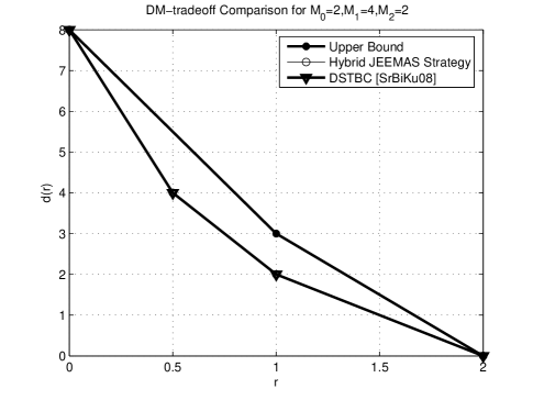
Figure 2: DM-tradeoff comparison of hybrid JEEMAS with the strategy of [15]

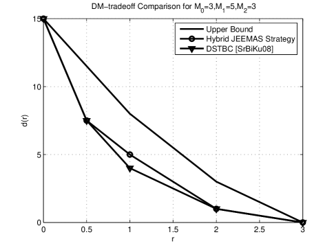
Figure 3: DM-tradeoff comparison of hybrid JEEMAS with the strategy of [15]

For the case when $\beta_{n}=0,\ \forall\ n$, the achievable DM-tradeoff of our hybrid JEEMAS strategy matches with that of the partitioning strategy of [15]. For the case when $\beta_{n}\neq 0,\ \forall\ n$, however, it is difficult to compare the hybrid JEEMAS strategy with the strategy of [15] in terms of achievable DM-tradeoff, since an optimization problem has to be solved for the strategy of [15]. For a particular example of $N=2,M_{0}=3,M_{1}=5,M_{2}=3$ the hybrid JEEMAS strategy outperforms the strategy of [15] as illustrated in Fig. 3. Moreover, in [15] a new partition is required for each $r$, in contrast to our strategy, which has only two modes of operation, one for $r=0$ and the other for $r>0$.

The following remarks are in order.

Remark 5

Recall that we assumed that $|S_{k_{n}}|=m$; i.e. equal number of antennas are selected at each relay stage. The justification of this assumption is as follows. Let us assume that $M_{n},\ n=0,1,\ldots,N$ antennas are used from each relay stage. Now assume that all relay stages are using the same number of antennas $M_{n}=m,\ \forall\ n,\ n\neq l$, except $l$, which is using $k$ antennas, $M_{l}=k$, and $m\neq k$. Using (9), it can be shown that the achievable DM-tradeoff with $M_{n}=m,\forall\ n,n\neq l$, and $M_{l}=k$ is a subset of the union of the achievable DM-tradeoff’s with using $M_{n}=m,\forall\ n$ (all relay stages using $m$ antennas), and $M_{n}=k,\forall\ n$ (all relay stages using $k$ antennas). Thus, it is sufficient to consider same number of antennas from each relay stage. It turns out, however, that different values of $m$ provide with different achievable DM-tradeoff’s because of the different number of independent paths in the multi-hop relay channel. To optimize over all possible values of $m$ we keep $m$ as a variable, and choose $m$ to obtain the best achievable DM-tradeoff.

Remark 6

Using the DM-tradeoff analysis of the JEEMAS strategy, we can obtain the DM-tradeoff of an antenna selection strategy for the point to point MIMO channel by considering a multi-hop relay channel with $N=0$, $M_{t}$ transmit, and $M_{r}$ receive antennas such that ($M_{t}\geq M_{r}$). Surprisingly we could not find this result in the literature and provide it here for completeness sake. Let $M_{t}=\alpha M_{r}+\beta$, and the transmitter uses $M_{r}$ antennas out of $M_{t}$ antennas that have maximum mutual information at the destination, then the DM-tradeoff is given by

$$d(r)=\alpha(M_{r}-r)(M_{r}-r)+\left[(\beta-r)(M_{r}-r)\right]^{+},$$

$r=0,1,\ldots,M_{r}$. The proof follows directly from (9).

Remark 7

CSI Requirement: With the proposed hybrid JEEMAS strategy, the destination needs to feedback the index of the path with the maximum mutual information to the source and each stage. Recall from the derivation of the achievable DM-tradeoff of the JEEMAS strategy that only $\kappa$ paths in a multi-hop relay channel are independent, and control the achievable DM-tradeoff for $\beta_{n}=0,\ \forall\ n$. Thus, the destination only needs to feedback the index of the best path among $\kappa$ independent paths with the maximum mutual information. Consequently the destination only needs to know CSI for $\kappa$ paths. For the case when $\beta_{n}\neq 0,\ \forall\ n$, we need to consider one more path from partition ${\cal P}_{2}$ corresponding to $m$ and $\beta_{n}$ antennas of alternate relay stages. Thus, the CSI overhead is moderate for the proposed EEAS strategy.

Remark 8

Feedback Overhead: As explained in Remark 7, to obtain the achievable DM-tradeoff of the hybrid JEEMAS strategy it is sufficient to consider any one set of $\kappa$ or $\kappa+1$ independent paths. Let the destination choose a particular set $S$ of $\kappa+1$ independent paths. Then each relay node knows on which of the paths of $S$ it lies and depending on the index of the element of $S$ from the destination, it knows whether to transmit or remain silent. Thus, only $\log_{2}(\kappa+1)$ bits of feedback is required from the destination to the source and each stage. Therefore the feedback overhead with the proposed EEAS strategy is quite small and can be realized with a very low rate feedback link.

Discussion: In this section we proposed a hybrid JEEMAS strategy that has two modes of operation, one for $r=0$, where it uses a single antenna of each stage, and the other for $r>0$, that uses $\min_{n=0,\ldots,N}M_{n}$ antennas of each stage. The proposed strategy is shown to achieve both the corner points of the optimal DM-tradeoff curve, corresponding to the maximum diversity gain and the maximum multiplexing gain. For intermediate values of multiplexing gain, the diversity gain of our strategy is quite close to that of the upper bound. Even though our strategy does not meet the upper bound, we show that it outperforms the best known DSTBC strategy [15], with smaller complexity and possess several advantages over DSTBCs as described in [24]. In the next section we propose a distributed CF strategy to achieve the optimal DM-tradeoff of the $2$-hop relay channel.

V Distributed CF Strategy for $2$-Hop Relay Channel

In this section we consider a $2$-hop relay channel with multiple relay nodes in the presence of a direct path between the source and the destination. For this $2$-hop relay channel we propose a distributed compress and forward (CF) strategy to achieve the optimal DM-tradeoff. The signal model for this section is as follows. We consider a $2$-hop relay channel with $K$ relay nodes, where the $k^{th}$ relay has $m_{k}$ antennas, and $\sum_{k=1}^{K}m_{k}=M_{1}$. The source and destination are assumed to have $M_{0}$ and $M_{2}$ antennas, respectively. We assume that the source and each relay have an average power constraint of $P$ . Let the signal transmitted from the source be ${\mathbf{x}}$, and from the relay node $k$ be ${\mathbf{x}}_{k}$, respectively. Then,

$${\mathbf{y}} = \sqrt{\frac{{P}}{M_{0}}}{\mathbf{H}}_{sd}{\mathbf{x}}+\sum_{k=1}^{K}\sqrt{\frac{{P}}{m_{k}}}{\mathbf{G}}_{k}{\mathbf{x}}_{k}+{\mathbf{n}},$$

$${\mathbf{y}}_{k} = \sqrt{\frac{{P}}{M_{0}}}{\mathbf{H}}_{k}{\mathbf{x}}+\sum_{\ell=1,k\neq\ell}^{K}\sqrt{\frac{{P}}{m_{\ell}}}{\mathbf{F}}_{k\ell}{\mathbf{x}}_{\ell}+{\mathbf{n}}_{k},$$ (10)

where ${\mathbf{y}}$ is the received signal at the destination, and ${\mathbf{y}}_{k}$ is the signal received at relay $k$.

Previously in [28], the CF strategy of [29] has been shown to achieve the optimal DM-tradeoff of a $2$-hop relay channel with a single relay node ($K=1$) in the presence of direct path between the source and the destination. The result of [28], however, does not generalize to the case of $2$-hop relay channel with multiple relay nodes. The problem with multiple relay nodes is unsolved, since how multiple relay nodes should cooperate among themselves to help the destination decode the source message is hard to characterize. A compress and forward (CF) strategy for a $2$-hop relay channel with multiple relay nodes has been proposed in [31], which involves partial decoding of other relays messages at each relay and transmission of correlated information from different relay nodes to the destination using distributed source coding. The achievable rate expression obtained in [31], however, is quite complicated and cannot be computed easily in closed form.

The achievable rate expression of the CF strategy [31] is complicated because each relay node partially decodes all other relay messages. Partial decoding introduces auxillary random variables which are hard to optimize over. To allow analytical tractability, we simplify the strategy of [31] as follows. In our strategy each relay compresses the received signal from the source using Wyner-Ziv coding similar to [31], but without any partial decoding of any other relay’s message. The compressed message is then transmitted to the destination using the strategy of transmitting correlated messages over a multiple access channel [33]. Our strategy is a special case of CF strategy [31], since in our case the relays perform no partial decoding. Consequently our strategy leads to a smaller achievable rate compared to [31]. The biggest advantage of our strategy, however, is its easily computable achievable rate expression and its sufficiency in achieving the optimal DM-tradeoff as shown in the sequel. We refer to our strategy as distributed CF from hereon in the paper. Even though the relays do not perform any partial decoding in the distributed CF strategy, in the sequel we show that they still provide the destination with enough information about the source message to achieve the optimal DM-tradeoff. Before describing our distributed CF strategy and showing its optimality in achieving the optimal DM-tradeoff, we present an upper bound on the DM-tradeoff of the $2$-hop relay channel.

$$L_{s}=\det\left(\frac{P}{M_{0}}{\mathbf{H}}_{s}^{d}{\mathbf{H}}_{s}^{d{\dagger}}+\left[\begin{array}[]{cccc}{\mathbf{I}}_{M_{2}}&0&0&0\\ 0&\left({\hat{N}}_{1}+1\right){\mathbf{I}}_{m_{1}}&0&0\\ 0&0&\ddots&0\\ 0&0&0&\left({\hat{N}}_{K}+1\right){\mathbf{I}}_{m_{K}}\end{array}\right]\right),$$

Lemma 9

[14] The DM-tradeoff of a two-way relay channel is upper bounded by

$$d(r) \leq \min\{(M_{0}-r)(M_{1}+M_{2}-r),$$

$$(M_{0}+M_{1}-r)(M_{2}-r)\},$$

$r=0,1,\ldots,\min\{M_{0},M_{1}+M_{2},M_{0}+M_{1},M_{2}\}$.

Proof: Let us assume that all the relay nodes and the destination are co-located and can cooperate perfectly. This assumption can only improve $d(r)$. In this case, the communication model from the source to destination is a point to point MIMO channel with $M_{0}$ transmit antennas and $M_{1}+M_{2}$ receive antennas. The DM-tradeoff of this MIMO channel is $(M_{0}-r)(M_{1}+M_{2}-r)$, and since this point to point MIMO channel is better than our original $2$-hop relay channel, $d(r)\leq(M_{0}-r)(M_{1}+M_{2}-r)$. Next, we assume that the source is co-located with all the relay nodes and can cooperate perfectly for transmission to the destination. This setting is equivalent to a MIMO channel with $M_{0}+M_{1}$ transmit and $M_{2}$ receive antenna with DM-tradeoff $(M_{0}+M_{1}-r)(M_{2}-r)$. Again, this point to point MIMO channel is better than our original $2$-hop relay channel and hence $d(r)\leq(M_{0}+M_{1}-r)(M_{2}-r)$, which completes the proof.  ∎

To achieve this upper bound we propose the following distributed CF strategy. Let the rate of transmission from source to destination be $R$. Then the source generates $2^{nR}$ independent and identically distributed $x^{n}$ according to distribution $p(x^{n})=\prod_{i=1}^{n}p(x_{i})$. Label them $x(w),\ w\in[2^{nR}]$. The codebook generation, the relay compression and transmission remains the same as in [31], expect that no relay node decodes any other relay’s codewords, i.e. no partial decoding at any relay node. Relay node $k$ generates $2^{nR_{k}}$ independent and identically distributed $x_{k}^{n}$ according to distribution $p(x_{k}^{n})=\prod_{i=1}^{n}p(x_{ki})$ and labels them $x_{k}(s),\ s\in[2^{nR_{k}}]$, and for each $x_{k}(s)$ generates $2^{n{\hat{R}}}$ ${\hat{y}}_{k}$’s, each with probability $p({\hat{y}}_{k}|x_{k}(s))=\prod_{i=1}^{n}p({\hat{y}}_{ki}|x_{ki}(s))$. Label these ${\hat{y}}_{k}(z_{k}|s),s\in[2^{nR_{k}}]$ and $z_{k}\in[2^{n{\hat{R}}_{k}}]$ and randomly partition the set $[2^{n{\hat{R}}_{k}}]$ into $2^{nR_{k}}$ cells $S_{s},\ s\in[2^{nR_{k}}]$.

Encoding: A Block Markov encoding [29] together with Wyner-Ziv coding [30] is used by each relay. Let in block $i$ the message to send from the source be $w_{i}$, then the source sends $x(w_{i})$. Let the signal received by relay $k$ in block $i$ be $y_{k}(i)$. Then $y_{k}(i)$ is compressed to ${\hat{y}}_{k}(z_{ik})$ using Wyner-Ziv coding [30] where correlation among $y_{1},\ldots,y_{K}$ is exploited. Then relay $k$ determines the cell index $s_{ik}$ in which $z_{ik}$ lies and transmits $x_{k}(s_{ik})$ in block $i+1$. We consider transmission of $B$ blocks of $n$ symbols each from the source in which $B-1$ messages will be sent. Each message is chosen from $w\in[2^{nR}]$. Thus, as $B\rightarrow\infty$, for fixed $n$, rate $R\left(\frac{B-1}{B}\right)$ is arbitrarily close to $R$ [29]. In the first block, the relay has no information about $s_{0k}$ necessary for compression. In this case, however, any good sequence allows each relay to start block Markov encoding [29]. In the last block, the source is silent and only the relays transmit to destination.

Decoding: Backward decoding is employed at the destination. At the end of block $i$, the codeword sent by source in block $i-1$ is decoded. At the end of block $i$, the destination first decodes $x_{k}$ for each $k$ by looking for a jointly typical $x_{k}(s_{ik})$ and $y_{i}$. If $R_{k}\leq I({\mathbf{x}}_{k};{\mathbf{y}}|{\mathbf{x}}_{[K]/k})$, $x_{k}(s_{ik})$ can be decoding reliably. Next, given that $x_{k}$’s have been decoded correctly for each $k$, the destination tries to find a set ${\cal L}$ of $z_{1},\ldots,z_{K}$ such that $\left(x_{1}(s_{1}),\ldots,x_{K}(s_{K}),{\hat{y}_{1}}(z_{1}|s_{1}),\ldots,{\hat{y}_{K}}(z_{K}|s_{K}),y\right)$ is jointly typical. The destination declares that $z_{1},\ldots,z_{K}$ were the correctly sent codewords if $(z_{1},\ldots,z_{K})\in\left(S_{s_{1}}\times S_{s_{2}}\times\ldots\times S_{s_{K}}\right)\cap{\cal L}$. After decoding $x_{1}(s_{1}),\ldots,x_{K}(s_{K})$ and $z_{1},\ldots,z_{K}$ the destination decodes ${\hat{w}}$ if $\left(x(w),x_{1}(s_{1}),\ldots,x_{K}(s_{K}),{\hat{y}_{1}}(z_{1}|s_{1}),\ldots,{\hat{y}_{K}}(z_{K}|s_{K}),y\right)$ is jointly typical. With this distributed CF strategy,

$$R \leq I({\mathbf{x}};{\mathbf{y}},\hat{{\mathbf{y}}}_{1},\ldots,\hat{{\mathbf{y}}}_{K}|{\mathbf{x}}_{1},\ldots,{\mathbf{x}}_{K})$$ (11)

is achievable with the joint probability distribution

$$p(x)\left[\prod_{k=1}^{K}p(x_{k})p({\hat{y}}_{k}|x_{k},y_{k})\right]\times$$

$$p(y_{1}.\ldots,y_{K},y|x,x_{1},\ldots,x_{K}),$$

subject to

$$I(\hat{{\mathbf{y}}}_{\cal T};{\mathbf{y}}_{\cal T}|{\mathbf{x}}_{[K]}{\hat{\mathbf{y}}}_{{\cal T}^{C}}{\mathbf{y}})+\sum_{t\in{\cal T}}I(\hat{{\mathbf{y}}}_{t};{\mathbf{x}}_{[K]/{t}}|{\mathbf{x}}_{t})$$

$$\leq I({\mathbf{x}}_{{\cal T}};{\mathbf{y}}|{\mathbf{x}}_{{\cal T}^{C}}),\ \forall\ {\cal T}\subseteq[K],$$ (12)

where ${\mathbf{y}}_{\cal T}$, $\hat{{\mathbf{y}}}_{\cal T}$ are vectors with elements ${\mathbf{y}}_{t},\ \hat{{\mathbf{y}}}_{t},\ t\in{\cal T},\ {\cal T}\subseteq[K]$, respectively, ${\mathbf{x}}_{[K]}$ is the vector containing ${\mathbf{x}}_{1},{\mathbf{x}}_{2},\ldots,{\mathbf{x}}_{K}$, and ${\cal T}^{C}$ is the complement of ${\cal T}$, where ${\cal T}\subseteq[K]$. For more detailed error probability analysis we refer the reader to [31]. In the next Theorem we compute the outage exponents for (11) and show that they match with the exponents of the upper bound.

Theorem 10

CF strategy achieves the DM-tradeoff upper bound (Lemma 9).

Proof: To prove the Theorem we will compute the achievable DM-tradeoff of the CF strategy (11) and show that it matches with the upper bound.

To compute the achievable rates subject to the compression rate constraints for the signal model (10), we fix ${\hat{\mathbf{y}}}_{k}={\mathbf{y}}_{k}+{\mathbf{n}}_{qr}$, where ${\mathbf{n}}_{qk}$ is $m_{k}\times 1$ vector with covariance matrix ${\hat{N}}_{k}{\mathbf{I}}_{m_{k}}$. Also, we choose ${\mathbf{x}}$, and ${\mathbf{x}}_{k}$ to be complex Gaussian with covariance matrices $\frac{P}{M_{0}}{\mathbf{I}}_{M_{0}}$, and $\frac{P}{m_{k}}{\mathbf{I}}_{m_{k}}$, and independent of each other, respectively. Next, we compute the various mutual information expressions to derive the achievable DM-tradeoff of the CF strategy. By the definition of the mutual information

$$I({\mathbf{x}};{\mathbf{y}},\hat{{\mathbf{y}}}_{1},\ldots,\hat{{\mathbf{y}}}_{K}|{\mathbf{x}}_{1},\ldots,{\mathbf{x}}_{K})=$$

$$\ \ \ \ \ \ \ \ \ h({\mathbf{y}},\hat{{\mathbf{y}}}_{1},\ldots,\hat{{\mathbf{y}}}_{K}|{\mathbf{x}}_{1},\ldots,{\mathbf{x}}_{K})$$

$$\ \ \ \ \ \ \ \ \ -h({\mathbf{y}},\hat{{\mathbf{y}}}_{1},\ldots,\hat{{\mathbf{y}}}_{K}|{\mathbf{x}},{\mathbf{x}}_{1},\ldots,{\mathbf{x}}_{K}).$$

From (10),

$$h({\mathbf{y}},\hat{{\mathbf{y}}}_{1},\ldots,\hat{{\mathbf{y}}}_{K}|{\mathbf{x}}_{1},\ldots,{\mathbf{x}}_{K})=\log L_{s},$$ (13)

where $L_{s}$ is defined on the top of the page and ${\mathbf{H}}_{s}^{d}=\left[{\mathbf{H}}_{sd}\ {\mathbf{H}}_{1}\ldots{\mathbf{H}}_{K}\right]^{T}$. From (10),

$$h({\mathbf{y}},\hat{{\mathbf{y}}}_{1},\ldots,\hat{{\mathbf{y}}}_{K}|{\mathbf{x}},{\mathbf{x}}_{1},\ldots,{\mathbf{x}}_{K})=$$

$$\log\det\left(\left[\begin{array}[]{cccc}{\mathbf{I}}_{M_{2}}&0&0&0\\ 0&\left({\hat{N}}_{1}+1\right){\mathbf{I}}_{m_{1}}&0&0\\ 0&0&\ddots&0\\ 0&0&0&\left({\hat{N}}_{K}+1\right){\mathbf{I}}_{m_{K}}\end{array}\right]\right),$$

which implies

$$I({\mathbf{x}};{\mathbf{y}},\hat{{\mathbf{y}}}_{1},\ldots,\hat{{\mathbf{y}}}_{K}|{\mathbf{x}}_{1},\ldots,{\mathbf{x}}_{K})=$$

$$\ \ \ \ \log\frac{L_{s}}{({\hat{N}}_{1}+1)^{m_{1}}({\hat{N}}_{2}+1)^{m_{2}}\ldots({\hat{N}}_{K}+1)^{m_{K}}}.$$ (14)

Next, we compute the values of ${\hat{N}}_{k}$’s that satisfy the compression rate constraints (12). Note that in (12), we need to satisfy the constraints for each subset ${\cal T}\subseteq[K]$. Towards that end, first we consider the subsets ${\cal T}$ of the form ${\cal T}=\{k\},\ k=1,2,\ldots,K$, and obtain the lower bound on the quantization noise ${\hat{N}}_{k}$ needed to satisfy (12), that is not proportional to $P$ for each $k$. It is important to note that ${\hat{N}}_{k}$ should not be proportional to $P$, otherwise from (14) it can be concluded that our distributed CF strategy cannot achieve the optimal DM-tradeoff. In the sequel we will point out how to obtain ${\hat{N}}_{k}$ satisfying (12) for all subsets of $[K]$.

$$L_{s[K]/k}=\det\left(\frac{P}{M_{0}}{\mathbf{H}}_{k}{\mathbf{H}}_{k}^{{\dagger}}+\sum_{\ell=1,\ \ell\neq k}^{K}\frac{P}{m_{\ell}}{\mathbf{F}}_{\ell k}{\mathbf{F}}_{\ell k}^{{\dagger}}+({\hat{N}}_{k}+1){\mathbf{I}}_{m_{k}}\right)$$

$$L_{s{\hat{k}}}={\det\left(\left[\begin{array}[]{cc}\left({\hat{N}}_{k}+1\right){\mathbf{I}}_{m_{k}}&0\\ 0&{\mathbf{I}}_{M_{2}}\end{array}\right]+\frac{P}{M_{0}}[{\mathbf{H}}_{k}\ {\mathbf{H}}_{sd}]^{T}[{\mathbf{H}}_{k}^{{\dagger}}\ {\mathbf{H}}_{sd}^{{\dagger}}]\right)}$$

For ${\cal T}=\{k\}$, from (12), for each relay $k$, we need to satisfy

$$I(\hat{{\mathbf{y}}}_{k};{\mathbf{y}}_{k}|{\mathbf{x}}_{[K]}{\hat{\mathbf{y}}}_{[K]/k}{\mathbf{y}})+I(\hat{{\mathbf{y}}}_{k};{\mathbf{x}}_{[K]/{k}}|{\mathbf{x}}_{k})$$

$$\leq I({\mathbf{x}}_{k};{\mathbf{y}}|{\mathbf{x}}_{[K]/k}).$$ (15)

By definition

$$I({\mathbf{x}}_{k};{\mathbf{y}}|{\mathbf{x}}_{[K]/k})=h({\mathbf{y}}|{\mathbf{x}}_{[K]/k})-h({\mathbf{y}}|{\mathbf{x}}_{k}{\mathbf{x}}_{[K]/k}),$$

$$\ \ \ \ =\log\underbrace{\det\left(\frac{P}{M_{0}}{\mathbf{H}}_{sd}{\mathbf{H}}_{sd}^{{\dagger}}+\frac{P}{m_{k}}{\mathbf{G}}_{k}{\mathbf{G}}_{k}^{{\dagger}}+{\mathbf{I}}_{M_{2}}\right)}_{L_{skd}}$$

$$\ \ \ \ \ \ \ -\log\underbrace{\det\left(\frac{P}{M_{0}}{\mathbf{H}}_{sd}{\mathbf{H}}_{sd}^{{\dagger}}+{\mathbf{I}}_{M_{2}}\right)}_{L_{sd}}\ \text{using}\ (\ref{rxsigdmtfd}).$$ (16)

Similarly,

$$I(\hat{{\mathbf{y}}}_{k};{\mathbf{x}}_{[K]/{k}}|{\mathbf{x}}_{k})=h(\hat{{\mathbf{y}}}_{k}|{\mathbf{x}}_{k})-h(\hat{{\mathbf{y}}}_{k}|{\mathbf{x}}_{[K]/{k}}{\mathbf{x}}_{k}),$$

$$=\log L_{s[K]/k}-\log\underbrace{\det\left(\frac{P}{M_{0}}{\mathbf{H}}_{k}{\mathbf{H}}_{k}^{{\dagger}}+({\hat{N}}_{k}+1){\mathbf{I}}_{m_{k}}\right)}_{L_{sk}},$$ (17)

where $L_{s[K]/k}$ is defined on the top of the page.

$$I(\hat{{\mathbf{y}}}_{k};{\mathbf{y}}_{k}|{\mathbf{x}}_{[K]}{\hat{\mathbf{y}}}_{[K]/k}{\mathbf{y}})=h(\hat{{\mathbf{y}}}_{k},{\mathbf{y}}|{\mathbf{x}}_{[K]}{\hat{\mathbf{y}}}_{[K]/k})$$

$$\ \ \ \ \ \ \ \ \ \ \ \ \ \ \ \ \ \ \ \ \ \ \ \ \ \ \ \ -h({\mathbf{y}}|{\mathbf{x}}_{[K]}{\hat{\mathbf{y}}}_{[K]/k})-h(\hat{{\mathbf{y}}}_{k}|{\mathbf{y}}_{k}),$$

$$=\log L_{s{\hat{k}}}-\log\underbrace{\det\left(\frac{P}{M_{0}}{\mathbf{H}}_{sd}{\mathbf{H}}_{sd}^{{\dagger}}+{\mathbf{I}}_{M_{2}}\right)}_{L_{sd}}$$

$$\ \ -\log{\hat{N}}_{k}^{m_{k}},$$ (18)

where $L_{s{\hat{k}}}$ is defined on the top of the page.

From (16, 17, 18), to satisfy the compression rate constraints (15) we need

$${\hat{N}}_{k}^{m_{k}}\geq\frac{L_{s[K]/k}L_{s{\hat{k}}}}{L_{skd}L_{sk}}.$$ (19)

Note that both sides of (19) are functions of ${\hat{N}}_{k}$, however, the resulting ${\hat{N}}_{k}$ is not a function of $P$ or SNR similar to [28]. Recall that we have only considered the subsets of $[K]$ of the form ${\cal T}=\{k\}$. For the rest of the subsets also, we can show that the quantization noise ${\hat{N}}_{k}$ required to satisfy (12) is not proportional to $P$. The analysis follows similarly and is deleted for the sake of brevity. Thus, to satisfy (12), we can take the maximum of the ${\hat{N}}_{k}$ required for each subset ${\cal T}\subseteq[K]$ and use that to analyze the DM-tradeoff. Let the maximum ${\hat{N}}_{k}$ required to satisfy (12) be ${\hat{N}}_{max,k}$. Since ${\hat{N}}_{k}$ for each subset ${\cal T}\subseteq[K]$ is not proportional to $P$, ${\hat{N}}_{max,k}$ is also not proportional to $P$.

Then, using (11) and (14), we can compute the outage probability of the distributed CF as follows. From [1], to compute $d(r)$, it is sufficient to find the negative of the exponent of the SNR of outage probability at the destination, where outage probability $P_{out}(r\log{\textsf{SNR}})$, is defined as

$$P_{out}(r\log{\textsf{SNR}}) = P(R\leq r\log{\textsf{SNR}}).$$

From (11) and (14),

$$R=\log\frac{L_{s}}{({\hat{N}}_{max,1}+1)^{m_{1}}\ldots({\hat{N}}_{max,K}+1)^{m_{K}}}.$$ (20)

Let $L_{d}:=\log\det\left(\frac{P}{M_{0}}{\mathbf{H}}_{sd}{\mathbf{H}}_{sd}^{{\dagger}}+\sum_{k=1}^{M}\frac{P}{m_{k}}{\mathbf{G}}_{k}{\mathbf{G}}_{k}^{{\dagger}}+{\mathbf{I}}_{M_{2}}\right)$. Then choose $l_{k}\in{\mathbb{Z}}$ such that

$${\hat{N}}_{max,k}\leq l_{k}\left(\left(\frac{L_{s}}{L_{d}}\right)^{1/{M_{1}}}+1\right),\ \forall\ k.$$ (21)

It is possible to choose $l_{k}$’s that satisfy (21), since ${\hat{N}}_{max,K}$ is not proportional to $P$.

Then

$$P_{out}(r\log{\textsf{SNR}})=$$

$$\ \ \ P\left(\log\frac{L_{s}}{\prod_{k=1}^{K}l_{k}\left(\left(\frac{L_{s}}{L_{d}}\right)^{1/{M_{1}}}+1\right)^{m_{k}}}\leq r\log{\textsf{SNR}}\right),$$

$$=P\left(\log\frac{L_{s}}{\left(\left(\frac{L_{s}}{L_{d}}\right)^{1/{M_{1}}}+1\right)^{M_{1}}\prod_{k=1}^{K}l_{k}}\leq r\log{\textsf{SNR}}\right).$$

$$P_{out}(k\log{\textsf{SNR}})\stackrel{{\scriptstyle.}}{{=}}$$

$$\ \ P\left(\frac{L_{s}}{\left(\left(\frac{L_{s}}{L_{d}}\right)^{1/{M_{1}}}+1\right)^{M_{1}}}\leq\prod_{k=1}^{K}l_{k}{\textsf{SNR}}^{r}\right),$$

$$=P\left(\frac{\left(L_{s}\right)^{\frac{1}{M_{1}}}\left(L_{d}\right)^{\frac{1}{M_{1}}}}{\left(L_{s}\right)^{\frac{1}{M_{1}}}+\left(L_{d}\right)^{\frac{1}{M_{1}}}}\leq\prod_{k=1}^{K}l_{k}^{\frac{1}{M_{1}}}{\textsf{SNR}}^{\frac{r}{M_{1}}}\right),$$

$$=P\left(\frac{\left(L_{s}\right)^{\frac{1}{M_{1}}}\left(L_{d}\right)^{\frac{1}{M_{1}}}}{\left(L_{s}\right)^{\frac{1}{M_{1}}}+\left(L_{d}\right)^{\frac{1}{M_{1}}}}\leq{\textsf{SNR}}^{\frac{r}{M_{1}}}\right),$$

where the last equality follows since multiplying SNR by constant does not change the DM-tradeoff.

From here on we follow [28] to compute the exponent of the $P_{out}(r\log{\textsf{SNR}})$.

Let

$$L_{sl}=\det\left(\frac{P}{M_{0}}{\mathbf{H}}_{s}^{d}{\mathbf{H}}_{s}^{d{\dagger}}+\left[\begin{array}[]{ccccc}{\mathbf{I}}_{M_{2}}&0&0&0\\ 0&{\mathbf{I}}_{m_{1}}&0&0\\ 0&0&\ddots&0\\ 0&0&0&{\mathbf{I}}_{m_{K}}\end{array}\right]\right).$$

Then, from (13), $L_{sl}\leq L_{s}$, therefore using Lemma 2 [28], it follows that

$$P_{out}(r\log{\textsf{SNR}}) \leq P\left(\left(L_{sl}\right)^{\frac{1}{M_{1}}}\leq{\textsf{SNR}}^{\frac{r}{M_{1}}}\right)$$

$$+\ P\left(\left(L_{d}\right)^{\frac{1}{M_{1}}}\leq{\textsf{SNR}}^{\frac{r}{M_{1}}}\right),$$

$$= P\left(L_{sl}\leq{\textsf{SNR}}^{r}\right)$$

$$+\ P\left(L_{d}\leq{\textsf{SNR}}^{r}\right),$$

$$:= {\textsf{SNR}}^{-d_{1}(r)}+{\textsf{SNR}}^{-d_{2}(r)}.$$

Therefore, to lower bound the DM-tradeoff we need to find out the outage exponents $d_{1}(r)$ and $d_{2}(r)$ of $L_{sl}$ and $L_{s}$. Notice that, however, $\log\left(L_{sl}\right)$ is the mutual information between the source and the destination by choosing the covariance matrix to be $\frac{P}{M_{0}}{\mathbf{I}}_{M_{0}}$, and allowing all the relays and the destination to cooperate perfectly. From [1], choice of $\frac{P}{M_{0}}{\mathbf{I}}_{M_{0}}$ as the covariance matrix does not change the optimal DM-tradeoff, therefore, $d_{1}(r)=(M_{0}-r)(M_{1}+M_{2}-r)$. Similar argument holds for $\log\left(L_{d}\right)$, by noting that $\log\left(L_{d}\right)$ is the mutual information between the source and the destination if all the relays and the source were co-located and could cooperate perfectly, while using covariance matrix ${\mathbf{Q}}$, where

$${\mathbf{Q}}=\left[\begin{array}[]{cccc}\frac{P}{M_{0}}{\mathbf{I}}_{M_{0}}&0&0&0\\ 0&\frac{P}{m_{1}}{\mathbf{I}}_{m_{1}}&0&0\\ 0&0&\ddots&0\\ 0&0&0&\frac{P}{m_{K}}{\mathbf{I}}_{m_{K}}\end{array}\right].$$

Thus, $d_{2}(r)=(M_{0}+M_{1}-r)(M_{2}-r)$. Thus, the achievable DM-tradeoff with CF strategy meets the upper bound (Lemma 9).  ∎

Discussion: In this section we proposed a simplified version of the distributed CF strategy of [31] and showed that it can achieve the optimal DM-tradeoff for the $2$-hop relay channel for any number of relays. In our distributed CF strategy, each relay uses Wyner-Ziv coding to compress the received signal without any partial decoding of other relay messages. After compression, each relay transmits the message to the destination using the strategy for multiple access channel with correlated messages [33], since the relay compressed messages are correlated with each other. Even though the achievable rate with our strategy is smaller than the one obtained in [31] (because of no partial decoding at any relay), we show that it is sufficient to achieve the optimal DM-tradeoff. We prove the result by showing that the exponent of the outage probability of our strategy matches with the upper bound on the optimal DM-tradeoff, without requiring the compression noise constraints to be proportional to the SNR.

Generalizing our distributed CF strategy is possible for more than $2$-hop relay channel, however, computing the exponents of the outage probability of achievable rate and compression rate constraints is a non-trivial problem.

VI Conclusions

In this paper we considered the problem of achieving the optimal DM-tradeoff of the multi-hop relay channel. First, we proposed an antenna selection strategy called JEEMAS, where a subset of antennas of each relay stage is chosen for transmission that has the maximum mutual information at the destination. We showed that the JEEMAS strategy can achieve the maximum diversity gain and the maximum multiplexing gain in a multi-hop relay channel. Then we compared the DM-tradeoff performance of the JEEMAS strategy with the best known DSTBC strategy [15]. We observed that the DM-tradeoff of the JEEMAS is better than the DSTBCs [15], expect for the case when the number of antennas at each stage are divisible by the minimum of the antennas across all relay stages, in which case the DM-tradeoffs of JEEMAS and DSTBCs [15] match.

Next, we proposed a distributed CF strategy for the $2$-hop relay channel with multiple relay nodes and showed that it achieves the optimal DM-tradeoff. Our distributed CF strategy is a special case of the strategy proposed in [31], where the specializations are done to allow analytical tractability. We showed that if each relay transmits a compressed version of the received signal using Wyner-Ziv coding, it is sufficient to achieve the optimal DM-tradeoff. Our distributed CF strategy can be extended to more than $2$-hop relay channels, however, computing the outage probability exponents is a non-trivial problem.

References

- [1] L. Zheng and D. Tse, “Diversity and multiplexing: A fundamental tradeoff in multiple-antenna channels,” IEEE Trans. Inf. Theory, vol. 49, no. 5, pp. 1073–1096, May 2003.
- [2] J. Laneman and G. Wornell, “Distributed space-time-coded protocols for exploiting cooperative diversity in wireless networks,” IEEE Trans. Inf. Theory, vol. 49, no. 10, pp. 2415–2425, Oct. 2003.
- [3] J. Laneman, D. Tse, and G. Wornell, “Cooperative diversity in wireless networks: Efficient protocols and outage behavior,” IEEE Trans. Inf. Theory, vol. 50, no. 12, pp. 3062–3080, Dec. 2004.
- [4] R. Nabar, H. Bolcskei, and F. Kneubuhler, “Fading relay channels: performance limits and space-time signal design,” IEEE J. Sel. Areas Commun., vol. 22, no. 6, pp. 1099–1109, Aug. 2004.
- [5] J. Yindi and B. Hassibi, “Distributed space-time coding in wireless relay networks with multiple-antenna nodes, submitted,” IEEE Trans. Signal Process., 2004.
- [6] ——, “Distributed space-time coding in wireless relay networks,” IEEE Trans. Wireless Commun., vol. 5, no. 12, pp. 3524–3536, Dec. 2006.
- [7] C. Yang and J.-C. Belfiore, “Optimal space time codes for the MIMO amplify-and-forward cooperative channel,” IEEE Trans. Inf. Theory, vol. 53, no. 2, pp. 647–663, Feb. 2007.
- [8] S. Yiu, R. Schober, and L. Lampe, “Distributed space-time block coding for cooperative networks with multiple-antenna nodes,” in Computational Advances in Multi-Sensor Adaptive Processing, 2005 1st IEEE International Workshop on, 13-15 Dec. 2005, pp. 52–55.
- [9] S. Barbarossa and G. Scutari, “Distributed space-time coding strategies for wideband multihop networks: regenerative vs. non-regenerative relays,” in Acoustics, Speech, and Signal Processing, 2004. Proceedings. (ICASSP ’04). IEEE International Conference on, vol. 4, 17-21 May 2004, pp. iv–501–iv–504vol.4.
- [10] M. Damen and R. Hammons, “Distributed space-time codes: relays delays and code word overlays,” in ACM International Conference On Communications And Mobile Computing 2007, Honolulu, Hawaii, USA, 12-16 Aug. 2007, pp. 354–357.
- [11] F. Oggier and B. Hassibi, “An algebraic family of distributed space-time codes for wireless relay networks,” in IEEE International Symposium on Information Theory, 2006, July 2006, pp. 538–541.
- [12] J. Yindi and B. Hassibi, “Using orthogonal and quasi-orthogonal designs in wireless relay networks,” IEEE Trans. Inf. Theory, vol. 53, no. 11, pp. 4106–4118, Nov. 2007.
- [13] Y. Jing and H. Jafarkhani, “Network beamforming with channel means and covariances at relays,” IEEE International Conference on Communications, 2008. ICC ’08., pp. 3743–3747, May 2008.
- [14] S. Yang and J. Belfiore, “Diversity of MIMO multihop relay channels,” Aug. 2007, available on http://arxiv.org/PScache/arxiv/pdf/0708/0708. 0386v1.pdf.
- [15] K. Sreeram, S. Birenjith, and P. Vijay Kumar, “DMT of multi-hop cooperative networks - part II: Half-duplex networks with full-duplex performance,” IEEE Trans. Inf. Theory, submitted, Aug. 2008, available on http://arxiv.org.
- [16] R. Vaze and R. W. Heath Jr., “Maximizing reliability im multi-hop wireless networks,” in IEEE Int. Symposium on Information Theory (ISIT) 2008, Toronto, July 2008, pp. 11–15.
- [17] F. Oggier and B. Hassibi, “Code design for multihop wireless relay networks,” Oct. 2007, available on www.hindawi.com.
- [18] S. Peters and R. W. Heath Jr., “Nonregenerative MIMO relaying with optimal transmit antenna selection, accepted for publication in,” IEEE Signal Process. Lett., Jan. 2008, available on http://arxiv.org/abs/0801.3272.
- [19] A. Bletsas, A. Khisti, D. Reed, and A. Lippman, “A simple cooperative diversity method based on network path selection,” IEEE J. Sel. Areas Commun., vol. 24, no. 3, pp. 659–672, March 2006.
- [20] L. Zinan and E. Erkip, “Relay search algorithms for coded cooperative systems,” IEEE Global Telecommunications Conference, 2005. GLOBECOM ’05, vol. 3, 28 Nov.-2 Dec. 2005.
- [21] A. Ibrahim, A. Sadek, W. Su, and K. Liu, “Cooperative communications with relay selection: when to cooperate and whom to cooperate with?” available at http://www.ece.umd.edu/asalah/IbrahimRelaySelectionTWC.pdf.
- [22] C. K. Lo, S. Vishwanath, and R. Heath, Jr, “Relay subset selection in wireless networks using partial decode-and-forward transmission,” IEEE Trans. Veh. Technol., submitted, available on http://arxiv.org/PScache/arxiv/pdf/0711/0711.3205v1.pdf 2007.
- [23] R. Tannious and A. Nosratinia, “Spectrally-efficient relay selection with limited feedback,” IEEE J. Sel. Areas Commun., vol. 26, no. 8, pp. 1419–1428, Oct. 2008.
- [24] R. Vaze and R. Heath, Jr, “To code or not to code in multi-hop relay channels,” IEEE Trans. Signal Process., accepted for publication Jan. 2009, available on http://arxiv.org.
- [25] M. Park, J. Andrews, and S. Nettles, “Wireless channel-aware ad hoc cross-layer protocol with multiroute path selection diversity,” Vehicular Technology Conference VTC 2003-Fall. 2003 IEEE 58th, vol. 4, pp. 2197–2201 Vol.4, 6-9 Oct. 2003.
- [26] B. Gui, L. Dai, and L. Cimini, “Routing strategies in broadband multihop cooperative networks,” 41st Annual Conference on Information Sciences and Systems, 2007. CISS ’07., pp. 661–666, 14-16 March 2007.
- [27] S. Bohacek, “Performance improvements provided by route diversity in multihop wireless networks,” IEEE Trans. Mobile Comput., vol. 7, no. 3, pp. 372–384, March 2008.
- [28] M. Yuksel and E. Erkip, “Multiple-antenna cooperative wireless systems: A diversity-multiplexing tradeoff perspective,” IEEE Trans. Inf. Theory, vol. 53, no. 10, pp. 3371–3393, Oct. 2007.
- [29] T. Cover and A. El Gamal, “Capacity theorems for relay channels,” IEEE Trans. Inf. Theory, vol. 25, no. 5, pp. 572–584, Sept. 1979.
- [30] A. Wyner and J. Ziv, “The rate-distortion function for source coding with side information at the decoder,” IEEE Trans. Inf. Theory, vol. 22, no. 1, pp. 1–10, Jan 1976.
- [31] G. Kramer, M. Gastpar, and P. Gupta, “Cooperative strategies and capacity theorems for relay networks,” IEEE Trans. Inf. Theory, vol. 51, no. 9, pp. 3037–3063, Sept. 2005.
- [32] T. Cover and J. Thomas, Elements of Information Theory. John Wiley and Sons, 2004.
- [33] T. Cover, A. Gamal, and M. Salehi, “Multiple access channels with arbitrarily correlated sources,” IEEE Trans. Inf. Theory, vol. 26, no. 6, pp. 648–657, Nov 1980.