Electrodynamic Casimir Effect in a Medium-Filled Wedge II

Abstract

We consider the Casimir energy in a geometry of an infinite magnetodielectric wedge closed by a circularly cylindrical, perfectly reflecting arc embedded in another magnetodielectric medium, under the condition that the speed of light be the same in both media. An expression for the Casimir energy corresponding to the arc is obtained and it is found that in the limit where the reflectivity of the wedge boundaries tends to unity the finite part of the Casimir energy of a perfectly conducting wedge-shaped sheet closed by a circular cylinder is regained. The energy of the latter geometry possesses divergences due to the presence of sharp corners. We argue how this is a pathology of the assumption of ideal conductor boundaries, and that no analogous term enters in the present geometry.

The Casimir effect casimir48 may be understood as an effect of the fluctuations of the quantum vacuum. Casimir’s original geometry involved two infinite and parallel ideal metal planes which were found to attract each other with a negative pressure scaling quartically with the inverse interplate separation. In a seminal paper, Lifshitz generalised Casimir’s original calculation to imperfectly reflecting plates lifshitz55 . Since its feeble beginnings research on the Casimir effect has grown from being of peripheral interest to a few theorists to a bustling field of research both experimental and theoretical with publications numbering in the hundreds each year. Recent reviews include BookMilton01 ; milton04 ; lamoreaux05 ; buhmann07 .

Progress on Casimir force calculations for other geometries has been slower in coming. Spherical and cylindrical geometries have naturally been objects of focus, the latter of direct interest to the effort reported herein. Only in 1981 was the Casimir energy of an infinitely long perfectly conducting cylindrical shell calculated deraad81 and the more physical but also significantly more involved case of a dielectric cylinder was considered only in recent years brevik94 ; gosdzinsky98 ; milton99 ; lambiase99 ; caveroPelaez05 ; romeo05 ; brevik07 . We might also mention recent work on the cylinder defined by a $\delta$-function potential, a so-called semitransparent cylinder caveroPelaez06 ; for weak-coupling, both the semitransparent cylinder and the dielectric cylinder have vanishing Casimir energy.

Closely related to the cylindrical geometry is the infinite wedge. The problem was first approached in the late seventies dowker78 ; deutsch79 as part of the still ongoing debate about how to interpret various divergences in quantum field theory with sharp boundaries. Since, various embodiments of the wedge have been treated by Brevik and co-workers brevik96 ; brevik98 ; brevik01 and others nesterenko02 ; razmi05 . A review may be found in BookMostepanenko97 . A wedge intercut by a cylindrical shell was considered by Nesterenko and co-workers, first for a semi-cylinder nesterenko01 , then for arbitrary opening angle nesterenko03 , and the corresponding local stresses were studied by Saharian rezaeian02 ; saharian07 ; saharian09 . The group at Los Alamos studied the interaction of an atom with a wedge mendes08 ; rosa08 previously investigated by Barton barton87 and others skipsey05 ; skipsey06 , the geometry realised in an experiment by Sukenik et al. some years ago sukenik93 . A recent calculation of the Casimir energy of a magnetodielectric cylinder intercut by a perfectly reflecting wedge filled with magnetodielectric material was recently reported by the current authors brevik09 . Common to all of these theoretical efforts is the assumption that the wedge be bounded by perfectly conducting walls.

While until recently relatively few treatments of the vacuum energy of the wedge existed, the problem of calculating the diffraction of electromagnetic fields by a dielectric wedge within classical eletromagnetics is an old one and several powerful methods have been developed within this field. The Green’s function of the potential (Poisson) equation in the vicinity of a perfectly conducting wedge was found more than a century ago by Macdonald macdonald1895 and extended to the wave equation with a plane wave source by Sommerfeld sommerfeld1896 . Generalising Sommerfeld’s method, the first theoretical solution to the scattering problem involving a wedge of finite conductivity was found by Malyuzhinets in his PhD work malyuzhinetsThesis50 (see osipov99 for a review; cf. also osipov98 ).

A different method was proposed by Kontorovich and Lebedev in 1938 kontorovich38 and used by Oberhettinger to solve the Green’s function problem some time later oberhettinger54 . The method has been given attention in recent analytical and numerical studies of the diffraction problem osipov93 ; knockaert97 ; rawlins99 ; salem06 ; salem08 .

In the present effort we study the Casimir energy in a magnetodielectric wedge of opening angle $\alpha$ inside and outside a perfectly conducting cylindrical shell of radius $a$—See Fig. 1. The interior and exterior of the wedge are both filled with magnetodielectric material under the restriction of isorefractivity (or diaphanousness), that is, the index of refraction $n^{2}(\omega)=\epsilon(\omega)\mu(\omega)$ is the same everywhere for a given frequency. This condition is adopted because without it the problem is no longer separable and not readily solvable. Moreover, we suspect that nondiaphanous media will lead to divergences, at least in the absence of dispersion.

As a natural extension of the considerations in brevik09 we derive an expression for the free energy of such a system by use of the argument principle vankampen68 . (By free energy, we mean that bulk terms not referring to the circular arc boundary are subtracted.) The necessary dispersion relation provided by the electromagnetic boundary conditions at the wedge sides is derived in two different ways; by a standard route of expansion of the solutions in Bessel function partial waves and by use of the Kantorovich-Lebedev (KL) transform. (Still a third method, based on the Green’s function formulation, is sketched in the Appendix.) The corresponding boundary condition equation at the cylindrical shell is well known. These together allow us to sum the energy of the eigenmodes of the geometry satisfying eigenvalue equations for the frequency and azimuthal wave number $\nu$ by means of the argument principle.

There are important differences between the diaphanous geometry considered herein and the standard geometry of a perfectly conducting wedge. Assuming diaphanous electromagnetic boundary conditions, the interior and exterior wedge sectors are coupled and remain so also in the limit where the reflectivity of the wedge boundaries tends to unity (for example by letting $\epsilon\to\infty,\mu\to 0$ so that their product is constant). Assuming the wedge be perfectly conducting from the outset, however, the interior of the wedge is severed cleanly from its exterior at all frequencies, a significantly different situation.

The Casimir energy of the perfectly conducting wedge and magnetodielectric arc considered in brevik09 was found to possess an unremovable divergent term associated with the corners where the arc meets the wedge. This is a typical artifact of quantum field theory with non-flat boundary conditions (e.g. nesterenko02 ; nesterenko01 ; nesterenko03 ). We will argue in section II.2 that there is no such term present in the geometry considered herein, and that the direct generalisation of the finite part of the energy of the system considered in brevik09 to the present system is in fact the full regularised Casimir energy. The reason for this rests upon two unphysical effects of perfectly conducting boundary conditions at the wedge sides (the vanishing of the tangential components of the electric field there). Namely, such boundary conditions exclude the existence of an azimuthally constant TM mode, and divides space cleanly into an interior and exterior sector with no coupling allowed between modes in the two sectors. Moreover, for a wedge consisting of perfectly conducting thin sheets dividing space into two complementary wedges, the ideal conductor boundary conditions will count the azimuthally constant TE mode twice whereas with more realistic boundary conditions such as considered here, such a mode must be common to the both sectors, $0\leq\theta<2\pi$. In these two respects the perfectly conducting wedge differs from the diaphanous one, and put together these redefinitions provided by the diaphanous wedge exactly remove the divergent extra energy term found in brevik09 and previously in nesterenko03 .

We show numerically that except for the singular term, the energy of a perfectly conducting wedge closed by a magnetodielectric cylinder whose reflectivity tends to unity is regained in the limit where we let the wedge boundaries become perfectly reflecting.

I Boundary conditions and dispersion relations

We begin by considering in general the form of an expression of the energy of a diaphanous wedge inside and outside a cylindrical shell such as depicted in Fig. 1. We assume the cylindrical shell to be perfectly reflecting. Let the interior sector $-\alpha/2<\theta<\alpha/2$ have permittivity and permeability $\epsilon_{1}$ and $\mu_{1}$ relative to vacuum, and the corresponding values for the exterior sector $\pi\geq|\theta|>\alpha/2$ be $\epsilon_{2}$ and $\mu_{2}$ so that $\epsilon_{1}(\omega)\mu_{1}(\omega)=\epsilon_{2}(\omega)\mu_{2}(\omega)\equiv n^{2}(\omega)$. The cusp of the wedge is chosen to lie along the $z$ axis, which is also the center of the cylindrical shell, and the interfaces are found at $\theta=\pm\alpha/2$ and at $\rho=a$ ($\rho$ is the distance to the $z$ axis).

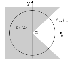
Figure 1: The wedge geometry considered.

We will calculate the Casimir energy by ‘summing’ over the eigenmodes of the geometry using the so-called argument principle, now a standard method in the Casimir literature. The eigenmodes of a given geometry are given by the solutions of the homogeneous Helmholtz equation

$$(\nabla^{2}-n^{2}\partial_{t}^{2})u(\mathbf{r},t)=0,$$ (1)

which also satisfy the system’s boundary conditions. Here $u$ symbolises a chosen field component of either the electric or magnetic field. We will choose $E_{z}$ and $H_{z}$ as the two independent field components from which the rest of the components can be derived by means of Maxwell’s equations.

The translational symmetry with respect to $z$ and time makes it natural to introduce the Fourier transform

$$E_{z}(\mathbf{r},t)=\int_{-\infty}^{\infty}\frac{d\omega}{2\pi}e^{-i\omega t}\int_{-\infty}^{\infty}\frac{dk_{z}}{2\pi}e^{ik_{z}z}E_{z}(\boldsymbol{\rho};\omega,k_{z}),$$

where $\boldsymbol{\rho}=(\rho,\theta)$ and $\rho=\sqrt{x^{2}+y^{2}}$. The Helmholtz equation now simplifies to the scalar Bessel equation

$$(\nabla^{2}_{\perp}+k_{\perp}^{2})E_{z}(\boldsymbol{\rho};k_{z},\omega)=0,$$ (2)

where

$$\nabla_{\perp}^{2}=\partial_{\rho}^{2}+\frac{1}{\rho}\partial_{\rho}+\frac{1}{\rho^{2}}\partial_{\theta}^{2}$$ (3)

and $k_{\perp}^{2}=\epsilon\mu\omega^{2}-k_{z}^{2}$.

We will define the quantity $\kappa$ as

$$\kappa=\sqrt{k_{z}^{2}-\epsilon\mu\omega^{2}}=-ik_{\perp},$$ (4)

where the root of $\kappa$ is to be taken in the fourth complex quadrant. When in the end we take frequencies to lie on the positive imaginary axis, $\kappa$ becomes real and positive, something we bear in mind in the subsequent calculations.

A general solution to Eq. (2) is of the form

$$E_{z}=[A_{\nu}H_{\nu}^{(1)}(k_{\perp}\rho)+B_{\nu}J_{\nu}(k_{\perp}\rho)](ae^{i\nu\theta}+be^{-i\nu\theta}),$$ (5)

where $A_{\nu},B_{\nu},a,b$ and $\nu$ are arbitrary. If, as in our case, $\nu$ is allowed to take non-integer values, we must restrict it to $\nu\geq 0$ because except at integers $J_{\nu}(z)$ and $J_{-\nu}(z)$ are linearly independent.

Solutions of the EM field in a wedge geometry are expressed as a sum over cylindrical partial waves whose kernel are Bessel and Hankel functions of argument $k_{\perp}\rho$. Thus it is clear that the boundary conditions on the wedge surfaces can only be solved for each partial wave if the speed of light is the same in both sectors since $k_{\perp}$ would otherwise take different values in the two media for given $k_{z}$ and $\omega$ and the kernel functions would be linearly independent functions of these. The diaphanous condition is thus prerequisite for the explicit solution of boundary conditions below. Without this condition the problem at hand is not analytically solvable with the methods used herein. We expect that even if we could solve the nondiaphanous problem we would encounter divergences that might or might not be curable by the inclusion of dispersion.

The presence of the wedge primarily has the rôle of dictating which values of $\nu$ are allowed. If one were to consider a cylinder (periodic boundary conditions), only integer values of $\nu$ (both positive and negative) would be acceptable and expressing the solution as a sum over these integer values would be appropriate. Were one instead to let the wedge be perfectly reflecting (Dirichlet and Neumann boundaries at $\pm\alpha/2$ where $\alpha$ is arbitrary) $\nu$ would be forced to take values that are non-negative integer multiples of $\pi/\alpha$. The diaphanous magnetodielectric boundaries present here also restrict $\nu$ to discrete values for given $\epsilon$’s and $\mu$’s, but explicitly determining these values is no longer immediate because modes existing in the exterior and interior sectors now couple to each other. For a given frequency we therefore make use of an appropriate dispersion function representing these boundaries in order to sum over the appropriate values of $\nu$ by means of the argument principle, whereupon we may sum over the eigenfrequencies of the modes inside and outside the cylindrical shell to obtain the energy.

The boundary condition dispersion relation pertaining to the circular boundary is known (e.g. brevik09 , Eq. (4.12), with $\xi^{2}=1$),

$$g_{\nu}(k_{z},\omega)\equiv 1-x^{2}\lambda_{\nu}^{2}(x)=0,$$ (6)

where $x=a\kappa$,

$$\lambda_{\nu}(x)=\frac{d}{dx}[I_{\nu}(x)K_{\nu}(x)],$$ (7)

$I_{\nu},K_{\nu}$ are the modified Bessel functions of the first and second kind of order $\nu$. We can simply use this equation to sum modes satisfying the boundary condition on both sides because the wedge boundaries at $\pm\alpha/2$ impose the same discretisation of $\nu$ inside and outside the cylindrical shell (were we to have e.g. a third medium in the sector $|\theta|<\alpha/2,\rho>a$ different from medium $1$, this would no longer be the case as we will see: the field solutions would take different values of $\nu$ inside and outside the cylindrical boundary and the boundary conditions at the cylinder could no longer be solved for each eigenvalue of $\nu$). We now turn to a derivation of the dispersion relation pertaining to the interfaces at $\theta=\pm\alpha/2$.

In the following we shall use the term TE to denote electromagnetic modes whose $\mathbf{E}$ field has no component in the $z$ direction and TM denotes those modes whose $\mathbf{H}$ field has no $z$ component. This is not ‘transverse electric’ and ‘transverse magnetic’ with respect to the wedge boundaries at $\theta=\pm\alpha/2$, but this does not matter since we will find that the eigenequation of these boundaries is the same for all field components by virtue of the diaphanous condition.

I.1 Kontorovich-Lebedev approach

We will first employ the technique of the Kontorovich-Lebedev (K-L) transformation kontorovich38 and its inverse transform which may be written as:

$$E_{z}(\boldsymbol{\rho})=$$

$$\mbox{\textgoth{E}}_{z}(\theta;\nu)= \frac{2}{\pi^{2}}\int_{0}^{\infty}\frac{d\rho}{\rho}e^{-\frac{i\nu\pi}{2}}K_{\nu}(\kappa\rho)E_{z}(\boldsymbol{\rho}),$$ (8a)

(dependence on $k_{z}$ and $\omega$ is implicit). While less extensively covered in the literature than most other integral transforms, some tables of K-L transforms exist BookDitkin65 ; BookOberhettinger72 . Numerical methods for evaluating such transforms were recently developed by Gautschi gautschi06 . We will ignore the presence of the cylindrical shell in this section and only study how the presence of the walls of the wedge discretize the spectrum of allowed values of the Bessel function order $\nu$.

With this, (2), after multiplying with $\rho^{2}$, transforms to

$$(\partial_{\theta}^{2}+\nu^{2})\mbox{\textgoth{E}}_{z}(\theta;\nu,k_{z},\omega)=0.$$ (8i)

Equation (8i) is now in a form fully analogous to that encountered in a planar geometry (e.g. schwinger78 ; ellingsen07 ; tomas95 ). We follow now roughly the scheme of tomas95 and determine the dispersion relation [condition for eigensolutions of Eq. (2)] by means of summation over multiple reflection paths. By noting that the solutions to Eq. (8i) have the form of propagating plane waves travelling clockwise or anticlockwise along the now formally straight $\theta$ axis ($\nu$ playing the role of a reciprocal azimuthal angle) the analogy to a plane parallel system is obvious.

We write the solution of Eq. (8i) in the interior sector, $|\theta|<\alpha/2$, in the form

$$\mbox{\textgoth{E}}_{z}=e^{+}e^{i\nu\theta}+e^{-}e^{-i\nu\theta},$$ (8j)

where $e^{\pm}$ are undetermined integration coefficients, field amplitudes at $\theta=0$ to be determined from boundary conditions at $\theta=\pm\alpha/2$.

Likewise the solutions in the exterior sector (the ‘complementary wedge’) $\pi\geq|\theta|>\alpha/2$ may be written

$$\tilde{\mbox{\textgoth{E}}}_{z}=\tilde{e}^{+}e^{i\nu(\theta-\pi)}+\tilde{e}^{-}e^{-i\nu(\theta-\pi)},$$ (8k)

where the undetermined amplitudes $\tilde{e}^{\pm}$ are ‘measured’ at $\theta=\pi$. The choice to measure the amplitudes in sectors 1 and 2 at $\theta=0$ and $\pi$ respectively is arbitrary, but makes for maximally symmetric boundary equations.

The homogeneous Helmholtz equation thus solves the scattered part of $\mbox{\textgoth{E}}_{z}$ given some source field $\mbox{\textgoth{E}}^{0}_{z}$. Let us assume there is a source field in form of an infinitely thin phased line source parallel to the $z$ axis at some position $\theta_{0}$ in the interior sector. The direct field (which only propagates away from the source) may be written in the form

$$\mbox{\textgoth{E}}_{z}^{0}=\Theta(\theta-\theta_{0})e_{0}^{+}e^{i\nu\theta}+\Theta(\theta_{0}-\theta)e_{0}^{-}e^{-i\nu\theta},$$ (8l)

where $\Theta(x)$ is the unit step function and the field amplitudes are “measured” at $\theta=0$. We do not need to know the constants $e_{0}^{\pm}$ explicitly and take these to be known constants. The multiple reflection problem (or equivalently, boundary condition problem) is now a system of four equations for the four amplitudes $e^{\pm},\tilde{e}^{\pm}$ as functions of $e_{0}^{\pm}$.

We define the reflection coefficients at the boundaries $\theta=\pm\alpha/2$ as the ratio of reflected vs. incoming field amplitude, $r=\mbox{\textgoth{E}}_{z,\text{refl}}/\mbox{\textgoth{E}}_{z,\text{in}}$, as seen by a wave coming from and reflected back into sector 1 (a wave going the opposite way experiences a coefficient $-r$). With the assumption $\epsilon_{1}\mu_{1}=\epsilon_{2}\mu_{2}$ the reflection coefficients of the $s$ and $p$ modes differ only by a sign:

$$r_{p}=\frac{\epsilon_{2}-\epsilon_{1}}{\epsilon_{2}+\epsilon_{1}}=-r_{s}=-\frac{\mu_{2}-\mu_{1}}{\mu_{2}+\mu_{1}}.$$ (8m)

We will simply use $r$ in the following, representing either of the modes. We also define the transmission coefficient, the ratio of the transmitted to the incoming amplitude, going from sector $i$ to sector $j$, $t_{ij}$ where $i,j=1,2$ denotes the sectors in figure 1,

$$t_{ij}\equiv t_{ij,s}=\frac{\mu_{j}}{\mu_{i}}\frac{2\epsilon_{j}}{\epsilon_{j}+\epsilon_{i}}=t_{ij,p}=\frac{2\mu_{j}}{\mu_{j}+\mu_{i}}.$$ (8n)

Since these coefficients are invariant under K-L transformation, they are the sought-after single interface reflection and transmission coefficients also in the K-L regime. Note that with the diaphanous condition, reflection coefficients are independent of $\nu$, something which would not be true in general. Were $r$ to depend on $\nu$ this would give rise to corrections to the energy expression derived in section II.1. (See also the Appendix, where such $\nu$ dependence does occur.)

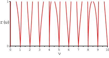
Figure 2: The solutions of the dispersion relation (I.1) as a function of $r$ and $\nu$ for $\alpha=0.75$. The eigenvalues of $\nu$ for a given $r$ are marked; the energy is calculated by summing over these values and then integrating over all $\omega$.

We formulate the electromagnetic boundary conditions in terms of reflection and transmission. In the K-L domain the system looks and behaves analogously to the planar system (see tomas95 for details on this case), but with one important difference, namely that a $\theta$ directed partial wave which is transmitted at a wedge boundary does not disappear from the system but is partly transmitted back into sector 1 again circularly. Thus we obtain four equations for the four amplitudes $e^{+},e^{-},\tilde{e}^{+}$ and $\tilde{e}^{-}$, coupling to each other through paths reflected or transmitted at one interface:

$$e^{+}= re_{0}^{-}e^{i\nu\alpha}+re^{-}e^{i\nu\alpha}+t_{21}\tilde{e}^{+}e^{i\nu\pi},$$ (8oa)

$$e^{-}= re_{0}^{+}e^{i\nu\alpha}+re^{+}e^{i\nu\alpha}+t_{21}\tilde{e}^{-}e^{i\nu\pi},$$ (8ob)

$$\tilde{e}^{+}= t_{12}e_{0}^{+}e^{i\nu\pi}+t_{12}e^{+}e^{i\nu\pi}-r\tilde{e}^{-}e^{i\nu(2\pi-\alpha)},$$ (8oc)

$$\tilde{e}^{-}= t_{12}e_{0}^{-}e^{i\nu\pi}+t_{12}e^{-}e^{i\nu\pi}-r\tilde{e}^{+}e^{i\nu(2\pi-\alpha)}.$$ (8od)

Eigenvalues of $\nu$ for the wedge correspond to solutions of these boundary conditions, which exist when the secular equation of the set of linear equations for $e^{\pm}$ and $\tilde{e}^{\pm}$ is fulfilled. The characteristic matrix is

$$\mathbf{D}=\left(\begin{array}[]{cccc}1&-re^{i\nu\alpha}&-t_{21}e^{i\nu\pi}&0\\ -re^{i\nu\alpha}&1&0&-t_{21}e^{i\nu\pi}\\ -t_{12}e^{i\nu\pi}&0&1&re^{i\nu(2\pi-\alpha)}\\ 0&-t_{12}e^{i\nu\pi}&re^{i\nu(2\pi-\alpha)}&1\end{array}\right)$$ (8t)

and the dispersion relation sought after is

$$D(\nu,\omega)\equiv\det\mathbf{D}=0.$$ (8u)

The matrix form (8t) is rather instructive. Note how $\mathbf{D}$ is a block matrix of the form

$$\mathbf{D}=\left(\begin{array}[]{cc}\mathbf{D}_{1}&\mathbf{G}_{21}\\ \mathbf{G}_{12}&\mathbf{D}_{2}\end{array}\right),$$

where $\mathbf{D}_{i}$ describes multiple scattering within sector $i$ and $\mathbf{G}_{ij}$ describes coupling between the sectors by transmission from sector $i$ to $j$. Since the $\mathbf{G}$ matrices commute with the $\mathbf{D}$ matrices, $\det\mathbf{D}$ can be written

$$\det\mathbf{D}=\det(\mathbf{D}_{1}\mathbf{D}_{2}-\mathbf{G}_{21}\mathbf{G}_{12}).$$ (8x)

We may use the energy conservation relation

$$t_{12}t_{21}+r^{2}=1,$$ (8y)

together with (8x) to find the simple expression

$$D(\nu,\omega)= (1-e^{2\pi i\nu})^{2}-r^{2}(e^{i\nu(2\pi-\alpha)}-e^{i\nu\alpha})^{2}$$

$$= -4e^{2\pi i\nu}[\sin^{2}(\nu\pi)-r^{2}\sin^{2}(\nu(\pi-\alpha))].$$ (8z)

It is noteworthy that this dispersion relation only has an implicit dependence on $\omega$ through the quantity $r^{2}(\omega)$. As an example we plot the solutions to Eq. (8u) as a function of $\nu$ and $r$ in Fig. 2 for $\alpha=0.75$ radians.

Note at this point that whenever $r$ is real, all zeros of $D(\nu,\omega)$ in (I.1) are real. In the following we shall think of $r$ as well as the eigenvalues of $\nu$ as real quantities. For real frequencies $\omega$ reflection coefficients will in general be complex, while after a standard rotation of frequencies onto the imaginary frequency axis these coefficients are always real as dictated by causality. Although zeros are complex the argument principle may still be used; the discussion of connected subtleties may be found in e.g. deraad81 ; brevik01b ; nesterenko06 .

It is easy to see that this dispersion relation generalises that for a cylinder (of infinite radius) and a perfectly conducting wedge. In the latter limit, $r=1$, the determinant $\det\mathbf{D}$ has zeros where $\nu=m\pi/\alpha$ and at $\nu=m\pi/(2\pi-\alpha)$ where $m$ is an integer. This becomes obvious when noting that

$$D(\nu,\omega)\buildrel r\to 1\over{\longrightarrow}-4e^{2\pi i\nu}\sin\nu\alpha\cdot\sin\nu(2\pi-\alpha).$$ (8aa)

This reproduces, in other words, the case where the wedge is made up of thin perfectly conducting sheets. For the perfectly conducting wedge it is customary to restrict $\nu$ to values that are integer multiples of $\pi/\alpha$ from the beginning.

Likewise when the two materials become equal,

$$D(\nu,\omega)\buildrel r=0\over{\longrightarrow}-4e^{2\pi i\nu}\sin^{2}\nu\pi\equiv D_{0}(\nu),$$ (8ab)

which has double zeros where $\nu=m$, a positive integer, corresponding to a clockwise and an anticlockwise mode or, if the reader prefers, the sum over $\nu=+m$ and $-m$. This is just the cylinder case deraad81 ; brevik94 ; gosdzinsky98 ; milton99 ; lambiase99 ; caveroPelaez05 ; romeo05 ; brevik07 . We see from Fig. 2 that except for $\nu=0$ which remains degenerate, the double zeroes split into two separate simple zeros for finite $r$. For special opening angles which are rational multiples of $\pi$ there will be other zeroes which remain degenerate as well.

One sees directly that were we to solve Eq. (2) for $H_{z}$ instead of $E_{z}$ the dispersion relation would be identical to Eq. (8u) since the only difference would be the sign of the reflection coefficient (we would employ $r_{s}$ rather than $r_{p}$), which only enters squared. One should note that the distinction between $r_{s}$ and $r_{p}$ here does not correspond to the distinction between TE and TM modes of the entire cavity, but this is of no consequence in the following because the dispersion relation (8u) is the same for all field components!

I.2 Derivation by standard expansion

We will now sketch how the result (I.1) may be derived by a more standard method similar to that made use of in brevik09 . The solutions of Eq. (5) that correspond to outgoing waves at $\rho\to\infty$ may be expanded following the scheme of brevik09 in an obvious generalisation of those found in BookStratton41 . Due to criteria of outgoing-wave boundary conditions at $\rho\to\infty$ and non-singularity at the origin the solution must consist purely of Hankel function $H^{(1)}_{\nu}(k_{\perp}\rho)$ far from the origin and only of terms containing $J_{\nu}(k_{\perp}\rho)$ near $\rho=0$. Following the scheme of brevik09 we choose $H_{\nu}^{(1)}(k_{\perp}\rho)$ for $\rho\geq a$ and $J_{\nu}(k_{\perp}\rho)$ for $\rho\leq a$ both in the interior sector $-\alpha/2<\theta<\alpha/2$ and outside, and couple the solutions across these straight boundaries. It will not matter which Bessel function we choose for the present purposes: the resulting solution expansions are identical but for the replacement of one Bessel function with another.

In a straightforward generalisation of the expansion used in brevik09 we write down the following general solutions in sector 1 of Fig. 1 for $\rho>a$:

$$E_{r,1}= \int_{0}^{\infty}d\nu\left\{\left[\frac{ik_{z}}{k_{\perp}}{H_{\nu}^{(1)}}^{\prime}\bar{a}_{1}-\frac{\nu\mu_{1}\omega}{k_{\perp}^{2}\rho}H_{\nu}^{(1)}\underline{b}_{1}\right]\cos\nu\theta+i\left[\frac{ik_{z}}{k_{\perp}}{H_{\nu}^{(1)}}^{\prime}\underline{a}_{1}-\frac{\nu\mu_{1}\omega}{k_{\perp}^{2}\rho}H_{\nu}^{(1)}\bar{b}_{1}\right]\sin\nu\theta\right\}e^{i\pi\nu/2},$$ (8aca)

$$E_{\theta,1}= -\int_{0}^{\infty}d\nu\left\{\left[\frac{\nu k_{z}}{k_{\perp}^{2}\rho}H_{\nu}^{(1)}\underline{a}_{1}+\frac{i\mu_{1}\omega}{k_{\perp}}{H_{\nu}^{(1)}}^{\prime}\bar{b}_{1}\right]\cos\nu\theta+i\left[\frac{\nu k_{z}}{k_{\perp}^{2}\rho}H_{\nu}^{(1)}\bar{a}_{1}+\frac{i\mu_{1}\omega}{k_{\perp}}{H_{\nu}^{(1)}}^{\prime}\underline{b}_{1}\right]\sin\nu\theta\right\}e^{i\pi\nu/2},$$ (8acb)

$$E_{z,1}= \int_{0}^{\infty}d\nu H_{\nu}^{(1)}\left[\bar{a}_{1}\cos\nu\theta+i\underline{a}_{1}\sin\nu\theta\right]e^{i\pi\nu/2},$$ (8acc)

$$H_{r,1}= \int_{0}^{\infty}d\nu\left\{\left[\frac{\nu\omega\epsilon_{1}}{k_{\perp}^{2}\rho}H_{\nu}^{(1)}\underline{a}_{1}+\frac{ik_{z}}{k_{\perp}}{H_{\nu}^{(1)}}^{\prime}\bar{b}_{1}\right]\cos\nu\theta+i\left[\frac{\nu\omega\epsilon_{1}}{k_{\perp}^{2}\rho}H_{\nu}^{(1)}\bar{a}_{1}+\frac{ik_{z}}{k_{\perp}}{H_{\nu}^{(1)}}^{\prime}\underline{b}_{1}\right]\sin\nu\theta\right\}e^{i\pi\nu/2},$$ (8acd)

$$H_{\theta,1}= \int_{0}^{\infty}d\nu\left\{\left[\frac{i\omega\epsilon_{1}}{k_{\perp}}{H_{\nu}^{(1)}}^{\prime}\bar{a}_{1}-\frac{\nu k_{z}}{k_{\perp}^{2}\rho}H_{\nu}^{(1)}\underline{b}_{1}\right]\cos\nu\theta+i\left[\frac{i\omega\epsilon_{1}}{k_{\perp}}{H_{\nu}^{(1)}}^{\prime}\underline{a}_{1}-\frac{\nu k_{z}}{k_{\perp}^{2}\rho}H_{\nu}^{(1)}\bar{b}_{1}\right]\sin\nu\theta\right\}e^{i\pi\nu/2},$$ (8ace)

$$H_{z,1}= \int_{0}^{\infty}d\nu H_{\nu}^{(1)}\left[\bar{b}_{1}\cos\nu\theta+i\underline{b}_{1}\sin\nu\theta\right]e^{i\pi\nu/2},$$ (8acf)

where we have omitted the arguments of $H_{\nu}^{(1)}(k_{\perp}\rho)$ and its derivative, and of $\bar{a}_{1}(\nu),\bar{b}_{1}(\nu)$, etc., the latter being undetermined coefficient functions of $\nu$.

We write the solution in sector 2 in exactly the same form but with the simple replacements $\theta\to\theta-\pi$ and $\epsilon_{1}\to\epsilon_{2},\mu_{1}\to\mu_{2}$ and the same for the coefficient functions. With the isorefractive assumption $k_{\perp}$ is the same in both media for given $\omega$ and $k_{z}$, so the boundary conditions at the interfaces can be solved under the integral signs. In general there are 8 unknown functions and eight equations, yet one finds that the $s$ and $p$ modes decouple into linear equation sets of $4\times 4$ on the form

$$\tilde{\mathbf{D}}\cdot\mathbf{a}=0$$ (8ad)

where $\tilde{\mathbf{D}}$ equals

$$\left(\begin{array}[]{cccc}\cos\frac{\nu\alpha}{2}&0&-\cos\nu(\frac{\alpha}{2}-\pi)&0\\ 0&\sin\frac{\nu\alpha}{2}&0&-\sin\nu(\frac{\alpha}{2}-\pi)\\ -\epsilon_{1}\sin\frac{\nu\alpha}{2}&0&\epsilon_{2}\sin\nu(\frac{\alpha}{2}-\pi)&0\\ 0&-\epsilon_{1}\cos\frac{\nu\alpha}{2}&0&\epsilon_{2}\cos\nu(\frac{\alpha}{2}-\pi)\end{array}\right)$$

and $\mathbf{a}$ is a vector, either $(\bar{a}_{1},\underline{a}_{1},\bar{a}_{2},\underline{a}_{2})$ or $(\bar{b}_{1},\underline{b}_{1},\bar{b}_{2},\underline{b}_{2})$.

As before the eigenmodes of the system solve the equation $\det\tilde{\mathbf{D}}=0$. With some manipulation we find that the determinant can be written simply as

$$\det\tilde{\mathbf{D}}= \frac{1}{4}(\epsilon_{2}-\epsilon_{1})^{2}\sin^{2}\nu(\pi-\alpha)$$

$$-\frac{1}{4}(\epsilon_{2}+\epsilon_{1})^{2}\sin^{2}\nu\pi.$$ (8ai)

Under the assumption that $\epsilon_{2}+\epsilon_{1}\neq 0$ the equation $\det\tilde{\mathbf{D}}=0$ is equivalent to Eq. (8u) with Eq. (I.1).

II The Casimir energy

In order to find the Casimir energy we shall employ the argument principle, introduced to the field of Casimir energy by van Kampen et al. vankampen68 who rederived Lifshitz’s result in a simple way. For a very readable review of the technique, see BookParsegian06 .

A similar system to that shown in Fig. 1 was considered in brevik09 where the plane sides of the wedge were instead made up of perfectly reflecting interfaces and the circular boundary was diaphanous. We will start from the result of brevik09 and generalise this step by step to approach the desired energy expression for the current situation. Excepting the formally singular energy term associated with the sharp corners where the arc meets the wedge walls found in that paper (we shall regard this term separately below), the Casimir energy per unit length of that system in the limit of perfectly reflecting circular arc was (Eq. (2.10) or (4.11) of brevik09 )

$$\tilde{\mathscr{E}}_{\text{id}}=\frac{1}{2\pi i}\int_{-\infty}^{\infty}\frac{dk_{z}}{2\pi}\sum_{m=0}^{\infty}\!{}^{{}^{\prime}}\oint_{\Lambda}d\omega\frac{\omega}{2}\frac{d}{d\omega}\ln g_{mp}(k_{z},\omega),$$ (8aj)

with $g_{\nu}(k_{z},\omega)$ given in Eq. (6) and we define the shorthand

$$p=\frac{\pi}{\alpha}.$$ (8ak)

The prime on the summation mark means the $m=0$ term is taken with half weight. The integration contour $\Lambda$ is chosen to follow the imaginary axis and is closed to the right by a large semicircle thus encircling the positive real axis. The roots of (6) are in general complex; the applicability of the argument principle for such situations was discussed in deraad81 ; brevik01b ; nesterenko06 ; nesterenko08 . The energy $\tilde{\mathscr{E}}$ has been normalised so as to be zero when the circular arc is moved to infinity.

Each frequency satisfying $g_{mp}(k_{z},\omega)=0$ gives a pole which adds the zero temperature energy $\frac{\omega}{2}$ of that mode through Cauchy’s integral theorem. In the end there are sums over the eigenvalues of $\nu$, $mp$, the eigenvalues found when the sides of the wedge are assumed to be perfectly conducting. Employing such an assumption from the start completely decouples the interior sector $|\theta|<\alpha/2$ from the exterior. If we were to interpret the perfectly reflecting wedge as the limit of an isorefractive wedge such as that described by the dispersion relation (I.1) as $|r|\to 1$, however (for example by letting $\epsilon_{2}\to\infty$ and $\mu_{2}\to 0$ so that their product is constant), the interior and exterior sectors remain coupled and we obtain an additional $m$-sum, namely that over $\nu=mp^{\prime}$ of the complementary wedge, where

$$p^{\prime}=\frac{\pi}{2\pi-\alpha}=\frac{p}{2p-1}.$$ (8al)

To obtain direct correspondence we therefore modify Eq. (8aj) by also including the energy of the modes of the complementary wedge, fulfilling $\nu=mp^{\prime}$. Since we will soon generalise this result to the case where the wedge is diaphanous, it is reasonable to subtract the energy corresponding to absence of the boundaries at $\pm\alpha/2$, by subtracting off the energy obtained were $\nu$ to fulfill periodic boundary conditions (i.e. a circular cylinder). The result is

$$\tilde{\mathscr{E}}_{\text{id}}\to\frac{1}{4\pi i}\int_{-\infty}^{\infty}\frac{dk_{z}}{2\pi}\sum_{m=0}^{\infty}\!{}^{{}^{\prime}}\oint_{\Lambda}d\omega\omega\frac{d}{d\omega}\ln\frac{g_{mp}\cdot g_{mp^{\prime}}}{g_{m}^{2}}.$$ (8am)

The periodic function $g_{m}(k_{z},\omega)$ is squared since both positive and negative integer orders contribute equally in the periodic case, and the symmetry under $m\to-m$ makes for a factor of 2 except for $m=0$. The latter exception is automatically accounted for by the prime on the sum.

Note that employing $g_{\nu}(k_{z},\omega)$ with the argument principle automatically takes care of the sum over the two polarisations since, by virtue of the diaphanous condition, $g_{\nu}$ is a product of boundary conditions for TE and TM modes (see e.g. Appendix B of brevik09 ).

Let us now perform the generalisation of Eq. (8am) to the present case. The sum over $\nu=mp$ and $mp^{\prime}$ may be generalised to a sum over the solutions of Eq. (8u) using the argument principle once more to count the zeros of Eq. (I.1), and the subtraction of the periodic modes in the absence of the boundary is performed by subtracting the solutions of $D_{0}(\nu)=0$ with $D_{0}$ from Eq. (8ab) (note that the zeros of $D_{0}$ are double, automatically giving the factor 2 manually introduced in Eq. (8am) by taking the square of $g_{m}$). We obtain

$$\tilde{\mathscr{E}}= \frac{1}{2(2\pi i)^{2}}\int_{-\infty}^{\infty}\frac{dk_{z}}{2\pi}\oint_{\Lambda}d\omega\omega$$

$$\times\oint_{\Lambda}d\nu\left[\frac{d}{d\omega}\ln g_{\nu}(k_{z},\omega)\right]\frac{d}{d\nu}\ln\frac{D(\nu,\omega)}{D_{0}(\nu)}.$$ (8an)

The contour of the $\nu$ integral is the same as that for the $\omega$ integral.

Neither of the contour integrals obtain contributions from the semicircular contour arcs so we are left with integrals over imaginary order and frequency. Performing substitutions $\omega=i\zeta$ and $\nu=i\eta$ we obtain

$$\tilde{\mathscr{E}}= \frac{1}{16\pi^{3}i}\int_{-\infty}^{\infty}dk_{z}\int_{-\infty}^{\infty}d\zeta\zeta$$

$$\times\int_{-\infty}^{\infty}d\eta\left[\frac{d}{d\zeta}\ln g_{i\eta}(k_{z},i\zeta)\right]\frac{d}{d\eta}\ln\frac{D(i\eta,i\zeta)}{D_{0}(i\eta)}.$$ (8ao)

This is the general form of the Casimir energy of the system presented herein.

To be very explicit about the regularisations performed: Eq. (8ao) is the energy of the geometry of Fig. 1, minus the energy when the cylinder is pushed to infinity (the double wedge alone), minus the renormalised energy of the cylinder relative to uniform space,

$$\tilde{\mathscr{E}}=(\mathscr{E}_{\olessthan}-\mathscr{E}_{<})-\tilde{\mathscr{E}}_{\circ},$$ (8ap)

where $\tilde{\mathscr{E}}_{\circ}$ is the $\zeta$-renormalised energy of a cylindrical shell (relative to uniform space) considered in milton99 , and $\olessthan,<$ symbolise the double wedge with and without the cylindrical shell. It is thus clear that the energy should vanish when either the cylindrical boundary tends to infinity ($\mathscr{E}_{\olessthan}\to\mathscr{E}_{<}$ and $\tilde{\mathscr{E}}_{\circ}\to 0$) or when the wedge becomes completely transparent ($\mathscr{E}_{\olessthan}-\mathscr{E}_{<}\to\tilde{\mathscr{E}}_{\circ}$).

The corresponding free energy at finite temperature $T$ is found by simply substituting the integral over $\zeta$ in Eq. (8ao) with the well known Matsubara sum over the frequencies $\zeta_{k}=2\pi kT$ where $k\in\mathbb{Z}$;

$$\int_{-\infty}^{\infty}d\zeta f(i\zeta)\to 2\pi T\sum_{k=-\infty}^{\infty}f(i\zeta_{k}).$$ (8aq)

We will not consider finite temperature numerically in the present effort.

II.1 Non-dispersive approximation

In order to proceed to producing numerical results we make the simplifying assumption that $r$ be approximately constant with respect to $\zeta$ over the important range of $\zeta$ values; $\frac{dr}{d\zeta}\approx 0$. This a version of the constant reflection coefficient model which was previously found to be useful for the planar geometry ellingsen09 . While it is true that for any real material, reflectivity must tend to zero at infinite frequency, the non-dispersive approximation is a useful one and allows a simpler expression to be derived. We will find below that the resulting Casimir energy expression is finite even when $r=1$ for all frequencies, except when $\alpha=0$ or $2\pi$. There is therefore no need to assume high-frequency transparency for the sake of finiteness in this case.

With this assumption we can easily perform a partial integration in $\zeta$. We note that, when $r$ is independent of $\nu$ as in the diaphanous case (see the Appendix for a situation where this is not so),

$$\frac{d}{d\eta}\left[\ln\frac{D}{D_{0}}\right]= \frac{\alpha\sinh\eta(2\pi-\alpha)-(2\pi-\alpha)\sinh\eta\alpha}{\sinh^{2}\eta\pi-r^{2}\sinh^{2}\eta(\pi-\alpha)}$$

$$\times\frac{r^{2}\sinh\eta(\pi-\alpha)}{\sinh\eta\pi},$$ (8ar)

which is now approximated as independent of $\zeta$ and $k_{z}$. It is then opportune to perform a change of integration into the polar coordinates

$$X=n\zeta=\kappa\cos\theta;~{}~{}~{}Y=k_{z}=\kappa\sin\theta,$$ (8as)

so that $X^{2}+Y^{2}=\kappa^{2}$ and

$$\int_{-\infty}^{\infty}dk_{z}\int_{-\infty}^{\infty}d\zeta f(a\kappa)=\frac{2\pi}{na^{2}}\int_{0}^{\infty}dxxf(x),$$ (8at)

where $x=a\kappa$ as before. We obtain after integrating by parts

$$\tilde{\mathscr{E}}=\frac{i}{8\pi^{2}na^{2}}\int_{-\infty}^{\infty}d\eta\frac{r^{2}\sinh\eta(\pi-\alpha)[\alpha\sinh\eta(2\pi-\alpha)-(2\pi-\alpha)\sinh\eta\alpha]}{\sinh\eta\pi[\sinh^{2}\eta\pi-r^{2}\sinh^{2}\eta(\pi-\alpha)]}\int_{0}^{\infty}dxx\ln[1-x^{2}\lambda_{i\eta}^{2}(x)].$$ (8au)

Despite appearances this expression is in fact real. This is because the dispersion function in the first integral is an odd function of $\eta$ while the real and imaginary parts of the logarithm are even and odd respectively (provided the appropriate branch of the logarithm is taken), hence the imaginary part of $\tilde{\mathscr{E}}$ vanishes under symmetrical integration. It is straightforward to write down the correction terms containing $\frac{dr}{d\zeta}$ or $\frac{dr}{d\nu}$ should the reader wish to do so. Such is necessary were one to study the role of dispersion on the energy; we shall not consider this herein—but see the Appendix for $dr/d\nu\neq 0$.

The energy expression (8au) has the reasonable properties of being zero at $\alpha=\pi$ and symmetrical under the substitution $\alpha\leftrightarrow 2\pi-\alpha$. We will study Eq. (8au) numerically in section III. We argue in the next subsection that Eq. (8ao) is the full Casimir energy of this system (after subtracting that of the cylinder alone). Thus the zero energy at $\alpha=\pi$ demonstrates a particular generalisation of the theorem of Ambjørn and Wolfram (ambjorn83 , stated in Eq. (2.49) of BookMilton01 ): the energy of a semi-circular compact diaphanous cylinder is half that of a full cylinder (there is an equal contribution from the exterior ‘half-cylinder’ so the difference is zero).

For large $\eta$ the term proportional to $\alpha$ in the big fraction in Eq. (8au) behaves for $\pi-\alpha>0$ as

$$\frac{d}{d\eta}\ln\frac{D}{D_{0}}\sim\frac{2\alpha r^{2}}{e^{2\alpha\eta}-r^{2}},$$ (8av)

with a similar behavior for the term proportional to $2\pi-\alpha$, and so is exponentially convergent. With perfect reflectivity Eq. (8au) is finite except when $\alpha$ equals $0$ or $2\pi$ when $|r|=1$.

II.2 No additional corner term

In the geometry considered in brevik09 , which differed from the present one primarily by the assumption that the wedge be perfectly conducting, the Casimir energy was found to possess a divergent term which could be associated with the corners where the arc meets the wedge sides. When the arc was instead made diaphanous it was shown that this term could be rendered finite by virtue of high frequency transparency as displayed by any real material boundary.

The energy (8ao) is the direct generalisation of the finite part of the energy of the system considered in brevik09 . We will argue that when the wedge is also diaphanous, this is indeed the full energy of the system, regularised by the subtraction of the energy of the cylinder alone (which in turn is regularised by subtracting the energy of uniform space).

Let us recapitulate how the divergent term in brevik09 came about. The zeta function regularised energy expression (Eq. (4.13) of brevik09 ) adds the $m=0$ modes of both polarisations with half weight. There should be no $m=0$ TM mode, however, because the perfectly conducting wedge forces any azimuthally constant electric field to have zero amplitude everywhere, thus the half-weight zero TM mode should be subtracted. Moreover, since for arbitrary opening angles only positive values of $m$ are allowed, the zero TE mode should be counted with full rather than half weight, and thus the correction term equals one half the $m=0$ energy of the TE mode minus one half that of the TM mode.

In contrast we are here not considering perfectly conducting wedge boundaries so the TM $m=0$ mode should be included. The question becomes whether the $\nu=0$ TE and TM modes have been counted with only half the weight they should. In a system such as ours the interior and exterior sectors are coupled and all allowed modes are modes satisfying boundary conditions of the whole double wedge. Thus there can be only one azimuthally constant mode for all $\theta$ (not one for each sector as one obtains for a perfectly conducting wedge-sheet) hence the zero mode should be counted once. This is exactly what is done in Eq. (8ao) because the dispersion function (I.1) has a double zero at $\nu=0$ cancelling the factor $1/2$. Hence no additional correction term is necessary and the use of dispersion relations with the argument principle automatically gives the full result.

In our numerical considerations reported in section III we find correspondence with the finite part of the energy reported in brevik09 when applied to two complementary wedges separated by a perfectly conducting sheet. Note how this correspondance is somewhat peculiar: In the energy expression of that reference the zero mode was counted with half weight where it should have been accounted for fully, but in adding the energy of the complementary wedge as in Eq. (8be) each of the complementary wedges contribute a half of the $m=0$ mode energy, amounting to the full energy when we insist that this mode be common to the whole system.

It is thus made clear how the divergent term found in nesterenko01 ; nesterenko03 ; brevik09 can be seen as a pathology of the ideal conductor boundary conditions at $\theta=\pm\alpha/2$ which (a) completely removes the azimuthally constant TM mode and (b) cleanly severs the connection between the interior and exterior of the wedge. Whether a similar term would appear – perhaps with a finite value – for a non-diaphanous wedge remains an open question, since the diaphanous condition employed herein is also a special case.

III Numerical investigation

It is useful to introduce the shorthand notation

$$\tilde{\mathscr{E}}=-\frac{1}{4\pi^{2}na^{2}}\int_{0}^{\infty}d\eta\left[\frac{d}{d\eta}\ln\frac{D}{D_{0}}\right]Y(\eta),$$ (8aw)

where $Y$ is the imaginary part of the integral over the logarithm in Eq. (8au),

$$Y(\eta)=\int_{0}^{\infty}dxx\arctan\frac{-x^{2}\Im\mathrm{m}\{\lambda^{2}_{i\eta}(x)\}}{1-x^{2}\Re\mathrm{e}\{\lambda^{2}_{i\eta}(x)\}},$$ (8ax)

where we take the argument of the logarithm to lie in $[-\frac{\pi}{2},\frac{\pi}{2}]$.

Near $x=0$ this integrand behaves like $x\sin(\ln x)$, oscillating increasingly fast. Techniques of rotating the integration path are restricted by the scarcity of methods for evaluating Bessel functions of general complex order, and will anyway come at the cost of making $\frac{d}{d\eta}\ln D/D_{0}$ oscillatory. For numerical purposes it is more useful to perform the substitution $x=e^{y}$:

$$Y(\eta)=\int_{-\infty}^{\infty}dye^{2y}\arctan\frac{-e^{2y}\Im\mathrm{m}\{\lambda^{2}_{i\eta}(e^{y})\}}{1-e^{2y}\Re\mathrm{e}\{\lambda^{2}_{i\eta}(e^{y})\}}.$$ (8ay)

For moderate values of $\eta$ this integrand is numerically manageable (there are $\mathscr{O}(4\eta)$ significant oscillations to integrate over), the remaining challenge being the evaluation of $\lambda_{i\eta}(x)$.

Figure 3: (a)Different methods of calculation used in different areas of the $x,\eta$ plane (see text). (b) The function $Y(\eta)$.

Rather than consider the complex function $I_{i\eta}(x)$ it is numerically useful to consider the real function

$$L_{i\eta}(x)=\frac{1}{2}[I_{i\eta}(x)+I_{-i\eta}(x)].$$ (8az)

When $\eta$ is real, $L_{i\eta}(x)=\Re\mathrm{e}I_{i\eta}(x)$. We find, using the Wronskian relation

$$\mathscr{W}[K_{\nu},I_{\nu}](x)=1/x$$ (8ba)

and relations between the two modified Bessel functions, that $\lambda_{i\eta}$ can be written as

$$\lambda_{i\eta}(x)=\frac{1}{x}+2K_{i\eta}^{\prime}(x)L_{i\eta}(x)-\frac{2i\sinh\eta\pi}{\pi}K_{i\eta}^{\prime}(x)K_{i\eta}(x)$$ (8bb)

For obtaining the right limit of the integrand near $\eta=0$ one may notice that $Y(\eta)$ for small $\eta$ is

$$Y(\eta)\sim-\eta\int_{0}^{\infty}dxx^{2}\frac{4K_{0}K_{1}(1-2xI_{0}K_{1})}{x^{2}-(1-2xI_{0}K_{1})^{2}}+\mathscr{O}(\eta^{2})$$

plus higher orders. Numerically one finds

$$Y(\eta)\sim 0.87442\eta+\mathscr{O}(\eta^{2}).$$ (8bc)

A complete algorithm for evaluating $K$ and $L$ for imaginary order and real argument was developed by Temme, Gil and Segura gil04 ; gil04a . Since we are only calculating products of Bessel functions and the methods for calculating one is much like that for another, the code performance could be increased significantly by reprogramming (we used programming language C#).

Different calculation methods are appropriate in different areas of the $x,\eta$ plane as shown in Fig. IIIa. For $K$ and $K^{\prime}$ we use Maclaurin type series expansion in region I in the figure (bounded by $\eta>0.044(x-3.1)^{1.9}+x-3.1$) and in regions II and III (bounded by $\eta<380(\frac{x-3}{2300})^{0.572}$) a method of continued fractions is used gil02 (the continued fractions method of BookPress92 may be used for imaginary orders also). No continued fractions method is available for $L$, but series expansions turn out to be more robust than for $K,K^{\prime}$; for $x<60$ (region II) Maclaurin series expansion is used, and asymptotic series expansion is used above this (region III). In the remaining area (region IV) Airy function type asymptotic expansions were used gil04 ; temme97 ; gil03 . In addition a fast method for evaluating complex gamma functions was necessary - we used that of Spouge spouge94 . The resulting algorithm was able to calculate $\lambda_{i\eta}(x)$ with at least eight significant digits on $x,\eta\in[0,100]$, more than sufficient for our purposes.

Because the calculation of $\lambda$ is rather elaborate we do not do the double integral (8aw) directly, but calculate a number of discrete values of $Y(\eta)$ and use spline interpolation to represent $Y$ in the integration over $\eta$, which then converges rapidly. The function $Y(\eta)$ is zero at $\eta=0$ and increases smoothly thence to approach a positive constant, obtained already at modest values of $\eta$, as plotted in Fig. IIIb. The factor $[\ln D/D_{0}]^{\prime}$ behaves as $e^{-2\eta\alpha}$ for large $\eta$ (assuming $\alpha<\pi$) assuring rapid convergence when $\alpha$ is not close to zero or $2\pi$.

In the limit $r^{2}\to 1$ we should obtain correspondence with brevik09 where the energy of a perfectly reflecting wedge closed by a diaphanous arc was considered. In this strong coupling case (the arc becoming perfectly reflecting) the energy of the sector inside the wedge only (modulo a singular term) was written on the form

$$\tilde{\mathscr{E}}_{\text{id}}=\frac{1}{8\pi na^{2}}e(p),$$ (8bd)

where the dimensionless function $e(p)$ is given in brevik09 , Eq. (4.22), and $p=\pi/\alpha$ as before. In the present case the modes in the interior and exterior sectors never decouple, even in the limit $r\to 1$ and Eq. (8au) thus calculates the energy of the whole system, regularised by subtracting the energy of free space, that is, by subtracting the result when the arc is moved to infinity (this is already implicitly subtracted by use of Eq. (6)) and the wedge boundaries become transparent. The energy to compare with is therefore on the form given in brevik09 where the energy of the complementary wedge is added and that of a cylinder subtracted. We can therefore write Eq. (8am) in the form $\tilde{\mathscr{E}}_{\text{id}}=\tilde{e}_{\text{id}}(p)/8\pi na^{2}$ where

$$\tilde{e}_{\text{id}}(p)=e(p)+e(p^{\prime})-2e(1),$$ (8be)

and $p^{\prime}$ was defined in (8al).

For our system the corresponding function is

$$\tilde{e}(p)=-\frac{2}{\pi}\int_{0}^{\infty}d\eta\left[\ln\frac{D}{D_{0}}\right]^{\prime}Y(i\eta;r).$$ (8bf)

We plot $\tilde{e}(p)$ as a function of $p$ and as a function of $\alpha$ in Fig. III. When $r\to 1$ full agreement with $\tilde{e}_{\text{id}}(p)$ of Eq. (8be) is obtained.

Figure 4: Above: The function $\tilde{e}(p)$ calculated for different $r$. Below: Same quantity, now plotted as a function of opening angle $\alpha$.

Conclusions

We have analysed the Casimir energy of a magnetodielectric cylinder whose cross section is a wedge closed by a circular arc under the restriction that the cylinder be diaphanous, i.e. that the speed of light be spatially uniform. We obtain an expression for the Casimir energy per unit length of the cylinder, regularised by subtraction of the energy of the wedge alone and the cylinder alone. The energy is then zero when the opening angle of the wedge, $\alpha$, equals $\pi$, it is symmetrical under the substitution $\alpha\leftrightarrow 2\pi-\alpha$, and it remains finite as $\alpha$ tends to zero or $2\pi$ except when the absolute reflection coefficients of the wedge boundaries equal unity.

A numerical investigation confirms that this generalises a previously known result for a perfectly conducting wedge closed by a diaphanous magnetodielectric arc in the limit where the arc becomes perfectly reflecting, except for a singular term present in that geometry which we argue does not present itself in the present configuration. This implies that the singular term found and discussed in brevik09 is an artefact of the use of ideal conductor boundary conditions and does not enter for a diaphanous wedge.

We mention finally that the diaphanous condition $\epsilon\mu=$ constant is an important simplifying element in the analysis. If this condition were given up, the problem would be very difficult to solve. As mentioned also in brevik09 , the effect is the same as that encountered in the Casimir theory of a solid ball: the condition of diaphanousness causes the divergent terms to vanish brevik82 . Analogously, when calculating the Casimir energy for a piecewise uniform string, the same effect turns up. If the velocity of sound (in this case sound replaces light) is the same $(=c)$ in in the different pieces of the string, then the theory works smoothly brevik90 . If this condition is relaxed, the problem becomes in practice intractable.

Appendix A Semitransparent wedge

In this appendix we sketch another way of deriving the azimuthal dependence, based on an analogous scalar model, in which the wedge is described by a $\delta$-function potential,

$$V(\theta)=\lambda_{1}\delta(\theta-\alpha/2)+\lambda_{2}\delta(\theta+\alpha/2).$$ (8bg)

This has the diaphanous property of preserving the speed of light both within and outside the wedge. We can solve this cylindrical problem in terms of the two-dimensional Green’s function $G$, which satisfies

$$\left[-\frac{1}{\rho}\frac{\partial}{\partial\rho}\rho\frac{\partial}{\partial\rho}+\kappa^{2}-\frac{1}{\rho^{2}}\frac{\partial^{2}}{\partial\theta^{2}}+\frac{V(\theta)}{\rho^{2}}\right]G(\rho,\theta;\rho^{\prime},\theta^{\prime})$$

$$\qquad=\frac{1}{\rho}\delta(\rho-\rho^{\prime})\delta(\theta-\theta^{\prime}).$$ (8bh)

This separates into two equations, one for the angular eigenfunction $\Theta_{\nu}(\theta)$

$$\left[-\frac{\partial^{2}}{\partial\theta^{2}}+V(\theta)\right]\Theta_{\nu}(\theta)=\nu^{2}\Theta_{\nu}(\theta),$$ (8bi)

leaving us with the radial reduced Green’s function equation,

$$\left[-\frac{1}{\rho}\frac{\partial}{\partial\rho}\rho\frac{\partial}{\partial\rho}+\kappa^{2}+\frac{\nu^{2}}{\rho^{2}}\right]g(\rho,\rho^{\prime})=\frac{1}{\rho}\delta(\rho-\rho^{\prime}).$$ (8bj)

The latter, for a Dirichlet arc at $\rho=a$, has the familiar solution,

$$g(\rho,\rho^{\prime}) = I_{\nu}(\kappa\rho_{<})K_{\nu}(\kappa\rho_{>})-I_{\nu}(\kappa\rho)I_{\nu}(\kappa\rho^{\prime})\frac{K_{\nu}(\kappa a)}{I_{\nu}(\kappa a)},$$ (8bka)

$$\qquad\qquad\quad\rho,\rho^{\prime}<a,$$

$$g(\rho,\rho^{\prime}) = I_{\nu}(\kappa\rho_{<})K_{\nu}(\kappa\rho_{>})-K_{\nu}(\kappa\rho)K_{\nu}(\kappa\rho^{\prime})\frac{I_{\nu}(\kappa a)}{K_{\nu}(\kappa a)},$$ (8bkb)

$$\qquad\qquad\quad\rho,\rho^{\prime}>a.$$

The azimuthal eigenvalue $\nu$ is determined by Eq. (8bi). For the wedge $\delta$-function potential (8bg) it is easy to determine $\nu$ by writing the solutions to Eq. (8bi) as linear combinations of $e^{\pm i\nu\theta}$, with different coefficients in the sectors $|\theta|<\alpha/2$ and $\pi\geq|\theta|>\alpha/2$. Continuity of the function, and discontinuity of its derivative, are imposed at the wedge boundaries. The four simultaneous linear homogeneous equations have a solution only if the secular equation is satisfied:

$$0=D(\nu) = \sin^{2}\nu(\alpha-\pi)-\left(1-\frac{4\nu^{2}}{\lambda_{1}\lambda_{2}}\right)\sin^{2}\pi\nu$$ (8bl)

$$\quad\mbox{}-\left(\frac{\nu}{\lambda_{1}}+\frac{\nu}{\lambda_{2}}\right)\sin 2\pi\nu.$$

Because we recognize that the reflection coefficient for a single $\delta$-function interface is $r_{i}=(1+2i\nu/\lambda_{i})^{-1}$, so

$$\Re\mathrm{e}r_{1}^{-1}r_{2}^{-1}=1-\frac{4\nu^{2}}{\lambda_{1}\lambda_{2}},\quad\Im\mathrm{m}r_{1}^{-1}r_{2}^{-1}=\frac{2\nu}{\lambda_{1}}+\frac{2\nu}{\lambda_{2}},$$ (8bm)

we see that this dispersion relation coincides with that in Eq. (I.1) when the reflection coefficient is purely real. Note that the $\nu=0$ root of Eq. (8bl) is spurious and must be excluded; there are no $\nu=0$ modes for the semitransparent wedge.

Now the full Green’s function can be constructed as

$$G(x,x^{\prime}) = \int\frac{d\omega}{2\pi}e^{-i\omega(t-t^{\prime})}\int\frac{dk}{2\pi}e^{ik(z-z^{\prime})}$$ (8bn)

$$\qquad\times\frac{1}{2\pi}\sum_{\nu}\Theta_{\nu}(\theta)\Theta_{\nu}^{*}(\theta^{\prime})g_{\nu}(\rho,\rho^{\prime}),$$

from which the Casimir energy per length can be computed from

$$\mathscr{E}=\frac{1}{2i}\int_{-\infty}^{\infty}\frac{d\omega}{2\pi}2\omega^{2}\int_{-\infty}^{\infty}\frac{dk}{2\pi}\sum_{\nu}\int_{0}^{\infty}d\rho\,\rho\,g_{\nu}(\rho,\rho),$$ (8bo)

where we have recognized that because the eigenvalue equation for $\nu$ is a Sturm-Liuoville problem, the integration over the $\theta$ eigenfunctions is $2\pi$. As above, we can enforce the eigenvalue condition by the argument principle, so we have the expression after again converting to polar coordinates as in Eq. (8as),

$$\mathscr{E}=\frac{1}{8\pi^{2}i}\int_{0}^{\infty}d\kappa\,\kappa^{3}\int_{-\infty}^{\infty}d\eta\left(\frac{d}{d\eta}\ln D(i\eta)\right)\int_{0}^{\infty}d\rho\,\rho\,g_{i\eta}(\rho,\rho).$$ (8bp)

Further, we must subtract off the free radial Green’s function without the arc at $r=a$, which then implies

$$\int_{0}^{\infty}d\rho\,\rho\,g_{i\eta}(\rho,\rho)\to\frac{a}{2\kappa}\frac{d}{d\kappa a}\ln[I_{i\eta}(\kappa a)K_{i\eta}(\kappa a)],$$ (8bq)

as well as remove the term present without the wedge potential:

$$D(\nu)\to\tilde{D}(\nu)=\frac{\lambda_{1}\lambda_{2}}{4\nu^{2}}\frac{D(\nu)}{\sin^{2}\pi\nu},$$ (8br)

leaving us with an expression for the Casimir energy analogous to Eq. (8au). This can be further simplified by noting that $\frac{d}{d\eta}\ln\tilde{D}(i\eta)$ is odd, which then yields the expression

$$\mathscr{E}=-\frac{1}{4\pi^{2}a^{2}}\int_{0}^{\infty}dx\,x\int_{0}^{\infty}d\eta\left(\frac{d}{d\eta}\ln\tilde{D}(i\eta)\right)\arctan\frac{K_{i\eta}(x)}{L_{i\eta}(x)},$$ (8bs)

where

$$K_{\mu}(x) = -\frac{\pi}{2\sin\pi\mu}\left[I_{\mu}(x)-I_{-\mu}(x)\right],$$ (8bta)

$$L_{\mu}(x) = \frac{i\pi}{2\sin\pi\mu}\left[I_{\mu}(x)+I_{-\mu}(x)\right],$$ (8btb)

where both $L_{i\eta}(x)$ and $K_{i\eta}(x)$ are real for real $\eta$ and $x$, and

$$I_{i\eta}(x)=\frac{\sinh\eta\pi}{\pi}[L_{i\eta}(x)-iK_{i\eta}(x)].$$ (8bu)

Details of the calculation of the Casimir energy for a semitransparent wedge will appear elsewhere.

References

- (1) H. B. G. Casimir, Proc. Kon. Ned. Akad. Wetensch. 51, 793 (1948).
- (2) E. M. Lifshitz, Zh. Eksp. Teor. Fiz. 29, 94 (1955) [Sov. Phys. JETP 2, 73 (1956)]
- (3) K. A. Milton The Casimir Effect: Physical Manifestations of the Zero-Point Energy (World Scientific, Singapore, 2001)
- (4) K. A. Milton, J. Phys. A: Math. Gen. 37, R209 (2004)
- (5) S. K. Lamoreaux, Rep. Prog. Phys. 68, 201 (2005)
- (6) S. Y. Buhmann and D.-G. Welsch, Prog. Quantum Electron. 31, 51 (2007)
- (7) L. L. DeRaad, Jr. and K. A. Milton, Ann. Phys. 186, 229 (1981)
- (8) I. Brevik and G. H. Nyland, Ann. Phys. 230, 321 (1994)
- (9) P. Gosdzinsky and A. Romeo, Phys. Lett. B 441, 265 (1998)
- (10) K. A. Milton, A. V. Nesterenko and V. V. Nesterenko, Phys. Rev. D 59, 105009 (1999)
- (11) G. Lambiase, V. V. Nesterenko and M. Bordag, J. Math. Phys. 40, 6254 (1999)
- (12) I. Cavero-Peláez and K. A. Milton, Ann. Phys. 320, 108 (2005); J. Phys. A. 39, 6225 (2006)
- (13) A. Romeo and K. A. Milton, Phys. Lett. B 621, 309 (2005); J. Phys. A 39, 6703 (2006)
- (14) I. Brevik and A. Romeo, Phys. Scripta 76, 48 (2007)
- (15) I. Cavero-Peláez, K. A. Milton and K. Kirsten, J. Phys. A 40, 3607 (2007)
- (16) J. S. Dowker and G. Kennedy, J. Phys. A 11, 895 (1978)
- (17) D. Deutsch and P. Candelas, Phys. Rev. D 20, 3063 (1979)
- (18) I. Brevik and M. Lygren, Ann. Phys. 251, 157 (1996)
- (19) I. Brevik, M. Lygren and V. Marachevsky, Ann. Phys. 267, 134 (1998)
- (20) I. Brevik, K. Pettersen, Ann. Phys. 291, 267 (2001)
- (21) V. V. Nesterenko, G. Lambiase and G. Scarpetta, Ann. Phys. 298, 403 (2002)
- (22) H. Razmi, S. M. Modarresi, Int. J. Theor. Phys. 44, 229 (2005).
- (23) V. M. Mostepanenko and N. N. Trunov, The Casimir Effect and Its Applications (Oxford University Press, Oxford, 1997).
- (24) V. V. Nesterenko, G. Lambiase and G. Scarpetta, J. Math. Phys. 42, 1974 (2001)
- (25) V. V. Nesterenko, I. G. Pirozhenko and J. Dittrich, Class. Quantum Grav. 20, 431 (2003)
- (26) A. H. Rezaeian and A. A. Saharian, Clas. Quant. Grav. 19, 3625 (2002)
- (27) A. A. Saharian, Eur. Phys. J. C 52, 721 (2007)
- (28) A. A. Saharian, in The Casimir Effect and Cosmology: A volume in honour of Professor Iver H. Brevik on the occasion of his 70th birthday S. Odintsov et al. (eds.) (Tomsk State Pedagogical University Press, 2008), p.87, preprint hep-th/0810.5207 .
- (29) T. N. C. Mendes, F. S. S. Rosa, A. Tenório and C. Farina, J. Phys. A 41 164029 (2008)
- (30) F. S. S. Rosa, T. N. C. Mendes, A. Tenório and C. Farina, Phys. Rev. A 78 012105 (2008)
- (31) G. Barton, Proc. R. Soc. London 410, 175 (1987)
- (32) S. C. Skipsey, G. Juzeliūnas, M. Al-Amri, and M. Babiker, Optics Commun. 254, 262 (2005)
- (33) S. C. Skipsey, M. Al-Amri, M. Babiker, and G. Juzeliūnas, Phys. Rev. A 73, 011803(R) (2006)
- (34) C. I. Sukenik, M. G. Boshier, D. Cho, V. Sandoghdar and E. A. Hinds, Phys. Rev. Lett. 70 560 (1993)
- (35) I. Brevik, S. Å. Ellingsen and K. A. Milton, Phys. Rev. E 79 041120 (2009)
- (36) H. M. Macdonald, Proc. Lond. Math. Soc. 26, 156 (1895)
- (37) A. Sommerfeld, Math. Ann. 47 317 (1896)
- (38) G. D. Malyuzhinets, Ph.D. Thesis, P. N. Lebedev Phys. Inst. Acad. Sci. USSR (1950)
- (39) A. V. Osipov and A. N. Norris, Wave Motion 29, 313 (1999)
- (40) A. V. Osipov and K. Hongo, Electromagnetics 18, 135 (1998)
- (41) M. J. Kontorovich and N. N. Lebedev, Zh. Exp. Theor. Fiz 8, 1192 (1938)
- (42) F. Oberhettinger, Commun. Pure & App. Math. 7, 551 (1954)
- (43) A. V. Osipov, Probl. Diff. Prop. Waves 25 173 (1993)
- (44) L. Knockaert, F. Olyslager and D. De Zutter, IEEE Trans. Antennas Propag. 45, 1374 (1997)
- (45) A. D. Rawlins, Proc. R. Soc. Lond. A 455, 2655 (1999)
- (46) M. A. Salem, A. H. Kamel and A. V. Osipov, Proc. R. Soc. A 462, 2503 (2006).
- (47) M. A. Salem and A. H. Kamel, Q. J. Mech. Appl. Math. 61, 219 (2008)
- (48) N. G. van Kampen, B. R. A. Nijboer and K. Schram K, Phys. Lett. 26A, 307 (1968)
- (49) V. A. Ditkin and A. P. Prudnikov, Integral Transforms and Operational Calculus (Oxford: Pergamon Press, 1965) Ch. 11
- (50) F. Oberhettinger, Tables of Bessel Transforms (Berlin: Springer, 1972) Ch. 5
- (51) W. Gautschi, BIT 46 21 (2006).
- (52) J. Schwinger, L. L. DeRaad, Jr. and K. A. Milton, Ann. Phys. 115, 1 (1978)
- (53) S. A. Ellingsen and I. Brevik, J. Phys. A 40, 3643 (2007)
- (54) M. S. Tomaš, Phys. Rev. A 51, 2545 (1995)
- (55) I. Brevik, B. Jensen, and K. A. Milton, Phys. Rev. D 64, 088701 (2001)
- (56) V. V. Nesterenko, J. Phys. A, 39, 6609 (2006)
- (57) J. A. Stratton, Electromagnetic Theory (New York: McGraw Hill, 1941) §9.15
- (58) V. A. Parsegian, Van Der Waals Forces (Cambridge: Cambridge Univ. Press, 2006) §L3.3
- (59) V. V. Nesterenko, J. Phys. A, 41, 164005 (2008)
- (60) S. Å. Ellingsen, in The Casimir Effect and Cosmology: A volume in honour of Professor Iver H. Brevik on the occasion of his 70th birthday S. Odintsov et al. (eds.) (Tomsk State Pedagogical University Press, Tomsk, Russia, 2008), p.45, preprint quant-ph/0811.4214.
- (61) J. Ambjørn and S. Wolfram, Ann. Phys. 147, 1 (1983)
- (62) A. Gil, J. Segura, N.M. Temme, ACM Trans. Math. Soft. 30 145 (2004)
- (63) A. Gil, J. Segura, N.M. Temme, ACM Trans. Math. Soft. 30 159 (2004)
- (64) A. Gil, J. Segura, N.M. Temme, J. Comp. Phys. 175 398 (2002)
- (65) W. Press et.al., Numerical Recipes 2nd ed. (Cambridge: Cambridge Univ. Press, 1992) §6.6
- (66) N.M. Temme, Num. Alg. 15 207 (1997)
- (67) A. Gil, J. Segura, N.M. Temme, J. Comp. App. Math. 153 225 (2003)
- (68) J.L. Spouge, SIAM J. Numer. Anal. 31 931 (1994)
- (69) I. Brevik and H. Kolbenstvedt, Ann. Phys. (N.Y.) 143, 179 (1982); 149, 237 (1983).
- (70) To our knowledge the first paper in this direction was I. Brevik and H. B. Nielsen, Phys. Rev. D 41, 1185 (1990). A survey is given by I. Brevik, A. A. Bytsenko, and B. M. Pimentel, in Theoretical Physics 2002 (Horizons in World Physics), edited by T. F. George and H. F. Arnoldus (Nova Science, New York, 2002).