Time-dependent barrier passage of Two-dimensional non-Ohmic damping system

Abstract

The time-dependent barrier passage of an anomalous damping system is studied via the generalized Langevin equation (GLE) with non-Ohmic memory damping friction tensor and corresponding thermal colored noise tensor describing a particle passing over the saddle point of a two-dimensional quadratic potential energy surface. The time-dependent passing probability and transmission coefficient are analytically obtained by using of the reactive flux method. The long memory aspect of friction is revealed to originate a non-monotonic $\delta$(power exponent of the friction) dependence of the passing probability, the optimal incident angle of the particle and the steady anomalous transmission coefficient. In the long time limit a bigger steady transmission coefficient is obtained which means less barrier recrossing than the one-dimensional case.

I INTRODUCTION

The problem of escape from a metastable states potential is ubiquitous in almost all scientific areas. A great amount of chemical events, such as chemical reactions, molecular diffusion, or collision of molecular systems, etc, can be modeled by a single barrier escape process within the framework of standard Brownian motion sbm1 ; sbm2 ; sbm3 . Although many other thoughts such as transition state theory TST1 ; TST2 ; TST3 and unimolecular rate theory urt1 ; urt2 ; urt3 , etc, still work, the celebrated landmark elucidation of this problem is the Kramers rate theory kramers . Where in his famous work, H. A. Kramers established a reaction rate formula which is applicable to all the cases from moderate to strong damping. The method he used to calculate the rate constant is conventional, namely, flux-over-populationFOP . However, we noticed, among the various theoretical concepts for rate calculation FOP ; MFPT , the method of reactive flux JCP-Bao ; rf1 ; rf2 is a most powerful and convenient way to follow. In its spirit, the initial conditions are assumed to be at the top of the barrier, which correspond to the ensemble of trajectories which start with identical initial conditions but experience different stochastic histories. The escape rate then can be calculated by investigating the various flux of particles passing the transition state at the saddle point. Achievements of its application in one-dimensional (1D) cases JCP-Bao ; rf1 ; rf2 has been witnessed in the past decades, but it has never been used in the study of higher dimensional systems.

The recent widespread interest in anomalous diffusion nsp1 ; nsp2 ; nsp3 has highlighted the critical role that it plays in characterizing a large group of nonstandard statistical physics. For which, the non-Ohmic model with a idiosyncratic power law frequency depending spectral density nonOhmic1 ; nonOhmic2 ; nonOhmic3 bears prominent consequences in describing a rich variety of frequency-dependent damping mechanism. Previous 1D studies on it have shown that in the non-Ohmic case, the friction of the system has a long time memory, the transmission coefficient of the system acts as a non-monotonic function of $\delta$(power exponent of the friction) which reveals a relatively strong recrossing phenomenon JCP-Bao ; nsp3 . But no higher dimensional study has occurred on this subject. However, a recent work by us has shown that in high dimensional systems, the non-diagonal correlation between various degrees of freedom will endow the barrier passage a riveting character Chyw , in particular, particles moving in a two-dimensional (2D) potential energy surface (PES) tend to select an optimal diffusion path to surmount the barrier. So it is of great interest to investigate the time-dependent barrier passage of high dimensional non-Ohmic damping systems.

The primary purpose of this paper is then to report our recent study on the non-Ohmic damping system. In Sec. II, the analytical expression of the saddle-point passing probability is obtained by solving the 2D coupled generalized Langevin equation with non-Ohimic friction tensor. In Sec. III, we give the time-dependent transmission coefficient derived by using of the reaction flux method. Sec. IV serves as a summary of our conclusion.

II 2D non-Ohmic passing probability

We consider the directional diffusion of a particle in the 2D quadratic PES: $U(x_{1},x_{2})=\frac{1}{2}\omega_{ij}x_{i}x_{j}$ with $i,j=1,2$ and $\det\omega_{ij}<0$, the motion of the particle is described by the generalized Langevin equation (GLE) with a non-Ohmic memory friction tensor:

$$m_{ij}\ddot{x}_{j}(t)+\int_{{0}}^{\infty}dt^{\prime}\beta_{ij}(t-t^{\prime})\dot{x}_{j}(t^{\prime})+\omega_{ij}x_{j}(t)=\xi_{i}(t),$$ (1)

where the Einstein summation convention is used and the components of the random force are assumed to be zero-mean and their correlations obey the fluctuation-dissipation theorem

$$\langle\xi_{i}(t)\xi_{j}(t^{\prime})\rangle = k_{{}_{B}}T\beta_{ij}(t-t^{\prime})$$ (2)

$$= \frac{2k_{{}_{B}}T}{\pi}\int_{0}^{\infty}d\omega\frac{J_{ij}(\omega)}{\omega}\cos\omega(t-t^{\prime}),$$

with $k_{{}_{B}}$ the Boltzmann constant, $T$ the temperature of the reservoir and $J_{ij}(\omega)$ takes the form of non-Ohmic spectral density $J_{ij}(\omega)=\gamma_{ij}(\omega/\omega_{r})^{\delta}$, where $\delta$ is the power exponent taking values between 0 and 2, $\gamma_{ij}$ is the friction constant, and $\omega_{r}$ denotes a reference frequency allowing for the damping constant $\gamma_{ij}$ to have the dimension of a viscosity at any $\delta$.

The initial condition of the particle is denoted as $x_{j}(0)=x_{j0}$ and $\dot{x}_{j}(0)=v_{j0}$, where $x_{10}<0$ and $v_{10}>0$. Assuming that $x_{1}$-axis is the transport direction [$\omega_{11}<0$], the reduced distribution function of the particle for $x_{1}$, when the variables $x_{2}(t)$, $v_{1}(t)$ and $v_{2}(t)$ are integrated out, can be written as:

$$W(x_{1},t;x_{{}_{10}},x_{{}_{20}},v_{{}_{10}},v_{{}_{20}})$$

$$\ \ \ \ \ \ \ \ \ =\frac{1}{\sqrt{2\pi}\sigma_{x_{1}}(t)}\textrm{exp}\left({-\frac{(x_{1}-\langle x_{1}(t)\rangle)^{2}}{2\sigma^{2}_{x_{1}}(t)}}\right).$$ (3)

Applying on it the Laplace transform technique to Eq.(1) we get $x_{1}(t)$ and its variance $\sigma^{2}_{x_{1}}(t)$ at any time

$$x_{1}(t) = \langle x_{1}(t)\rangle+\sum^{2}_{i=1}\int^{t}_{0}H_{i}(t-t^{\prime})\xi_{i}(t^{\prime})dt^{\prime},$$ (4)

$$\sigma^{2}_{x_{1}}(t) = \int^{t}_{0}dt_{1}H_{i}(t-t_{1})\int^{t_{1}}_{0}dt_{2}\langle\xi_{i}(t_{1})\xi_{j}(t_{2})\rangle H_{j}(t-t_{2}),$$

where the mean position of the particle along the transport direction is given by

$$\langle x_{1}(t)\rangle=\sum^{2}_{i=1}\left[C_{i}(t)x_{i0}+C_{i+2}(t)v_{i0}\right],$$ (6)

which relates to the initial position and velocity. The time-dependent factors in Eq.(6) according to the residual theorem are $C_{i}(t)=\mathcal{L}^{-1}[\textsl{F}_{i}(s)/\textsl{P}(s)]$ $(i=1\ldots 4)$ with exponential forms, the two response functions in Eqs.(4) and (II) read $\textsl{H}_{1}(t)=\mathcal{L}^{-1}[\textsl{F}_{5}(s)/\textsl{P}(s)]$ and $\textsl{H}_{2}(t)=\mathcal{L}^{-1}[\textsl{F}_{6}(s)/\textsl{P}(s)]$, where $\mathcal{L}^{-1}$ denotes the inverse Laplace transform. The expressions of $P(s)$ and $F_{i}(s)$ $(i=1,...,6)$ are written in the appendix.

The probability of passing over the saddle point [$x_{1}=x_{2}=0$] is always called the characteristic function $\chi(x_{{}_{10}},x_{{}_{20}},v_{{}_{10}},v_{{}_{20}};t)$ which can be determined mathematically by integrating Eq.(3) over $x_{1}$ from zero to infinity

$$\chi(x_{{}_{10}},x_{{}_{20}},v_{{}_{10}},v_{{}_{20}};t) = \int^{\infty}_{0}W(x_{1},t;x_{{}_{10}},x_{{}_{20}},v_{{}_{10}},v_{{}_{20}})dx_{1}$$ (7)

$$= \frac{1}{2}\textrm{erfc}\left(-\frac{\langle x_{1}(t)\rangle}{\sqrt{2}\sigma_{x_{1}}(t)}\right).$$

In the barrier surmounting process, the probability density function of the particle that is originally at one side of the barrier spreads in the phase space due to thermal fluctuation, and its center moves driven by its initial velocity. For large times, the probability of passing over the saddle point converges to a finite value depending on the initial position and velocity of the particle, and the other fraction of the particles goes to infinite along the opposite direction. This results in the characteristic function Eq.(7) to be a number which is equal to 1 for reactive trajectories and 0 for nonreactive trajectories. If we consider only the long time result of state transition induced by the particle diffusion, the stationary passing probability is of great important to rely on. Mathematically it is calculated by $P_{\textmd{pass}}=\lim_{t\to\infty}\frac{1}{2}\textmd{erfc}\left[-\langle x_{1}(t)\rangle/(\sqrt{2}\sigma_{x_{1}}(t))\right]$.

Figure 1: Stationary passing probability as a function of the incident angel for various $\delta$. The parameters used are $\omega_{12}=-0.5$, $m_{12}=0.6$, $\omega_{11}=-2.0$, $\omega_{22}=1.5$, $m_{11}=1.5$, $m_{22}=2.0$, $\gamma_{12}=1.0$, $\gamma_{11}=1.8$, $\gamma_{22}=1.2$, $\omega_{r}=1.0$, and the initial condition of the particle is set $x_{10}=-1.0$, $x_{20}=0$, $v_{0}=1.9$.

In Fig. 1, we plot the stationary passing probability as a function of the incident angel for various power exponents $\delta$. In the calculations here and following, we rescale all the variables so that the dimensionless unit such as $k_{B}=1.0$ is used. Each friction strength $\gamma_{ij}$ is fixed to be a constant independent of $\delta$, and the reference frequency $\omega_{r}=1.0$. It is seen from Fig. 1 that, the stationary passing probability of non-Ohmic case ($\delta=0.6$ or $\delta=1.8$) is not so large as the result of Ohmic case ($\delta=1.0$). This can be understood from the point of view of the particle’s critical velocity which corresponds to the condition: $\lim_{t\rightarrow\infty}\langle x_{1}(t)\rangle=0$. Supposing $v_{{}_{10}}=v_{{}_{0}}\textrm{cos}\phi$ and $v_{{}_{20}}=v_{{}_{0}}\textrm{sin}\phi$ are the two components of the particle’s velocity along two directions $x_{1}$ and $x_{2}$. The critical velocity for a particle reads:

$$v^{c}_{{}_{0}}=-\frac{C_{1}(\infty)x_{{}_{10}}+C_{2}(\infty)x_{{}_{20}}}{C_{3}(\infty)\textrm{cos}\phi+C_{4}(\infty)\textrm{sin}\phi}.$$ (8)

For the parameters in Fig.1, we obtain $v^{c}_{{}_{0}}|_{\delta=1.8}\cong 2.6417>v^{c}_{{}_{0}}|_{\delta=0.6}\cong 2.3477>v^{c}_{{}_{0}}|_{\delta=1.0}\cong 1.8426$ when the incident angle is set $\phi=0.258\textmd{rad}$. Thus we can see the particle of non-Ohmic damping system has a small passing probability.

It is also shown in Fig. 1 that, for each $\delta$ there exits a certain incident angle for the particle to reach a maximum stationary passing probability. This implies, for the 2D non-Ohmic damping system, an optimal incident angle (or an optimal diffusion path) still exists for the particle to surmount the PES, in accordance with the Ohmic case ($\delta=1.0$) we have studied Chyw . The optimal incident angle for a particle of 2D non-Ohmic damping system can also be determined by retrospect the minimum value of the critical velocity Eq. (8). After some algebra we find in the long time limit it can be expressed by the system parameters as

$$\psi=\textrm{arctan}\left(\frac{m_{12}(\hat{\beta}_{22}[s]\varepsilon+\omega_{22})-m_{22}(\hat{\beta}_{12}[s]\varepsilon+\omega_{12})}{m_{11}\textsl{F}_{5}(\varepsilon)+m_{12}\textsl{F}_{6}(\varepsilon)}\right).$$ (9)

where $\varepsilon$ is the largest analytical root of $P(s)=0$, $\hat{\beta}_{ij}[s]=\tilde{\gamma}_{ij}s^{\delta-1}$ is the Laplace transform of the friction kernel function and $\tilde{\gamma}_{ij}=\gamma_{ij}\omega_{r}^{1-\delta}\textrm{sin}^{-1}(\delta\pi/2)$ is namely the effective friction here.

Noticing that Eq. (9) implicitly implies the power exponent $\delta$. This means in the non-Ohmic damping case the optimal incident angle has an intimate relation to the friction of the system. In Fig. 2, the $\delta$ dependence of the optimal incident angle $\psi$ at various effective friction is plotted. It shows that $\psi$ evolves as a non-monotonic function of $\delta$. This implies that the barrier passage of the two-dimensional non-Ohmic damping system is intimately controlled by the friction. Particle facing different friction strength will select different optimal path in its barrier surmounting process.

For instance Fig. 3 gives a schematic illustration of the optimal incident angel for various power exponents $\delta$ at different friction strength. From which we can see, comparing with the Ohmic case (i.e. $\delta=1.0$), when the system friction strength is not so strong (straight lines in Fig. 3), the optimal incident angle of non-Ohmic case tends to approach zero from a clockwise direction at most values of $\delta$. However, if the system has a relatively strong friction (dashed lines in Fig. 3), the optimal incident angle of non-Ohmic case tends to approach zero from a anticlockwise direction. Since the direction of zero incident angle represents the valley direction of the PES, this implies the particle diffusion under the influence of non-Ohmic friction will has the probability of tracing along the valley passage. This is a meaningful prediction for the study of barrier escape problem. To deicide the relation between the system parameters that enables the particle to travel along the valley direction, one needs only set $\psi=0$. This will be very useful in studying the fusion reactions of massive nuclei.

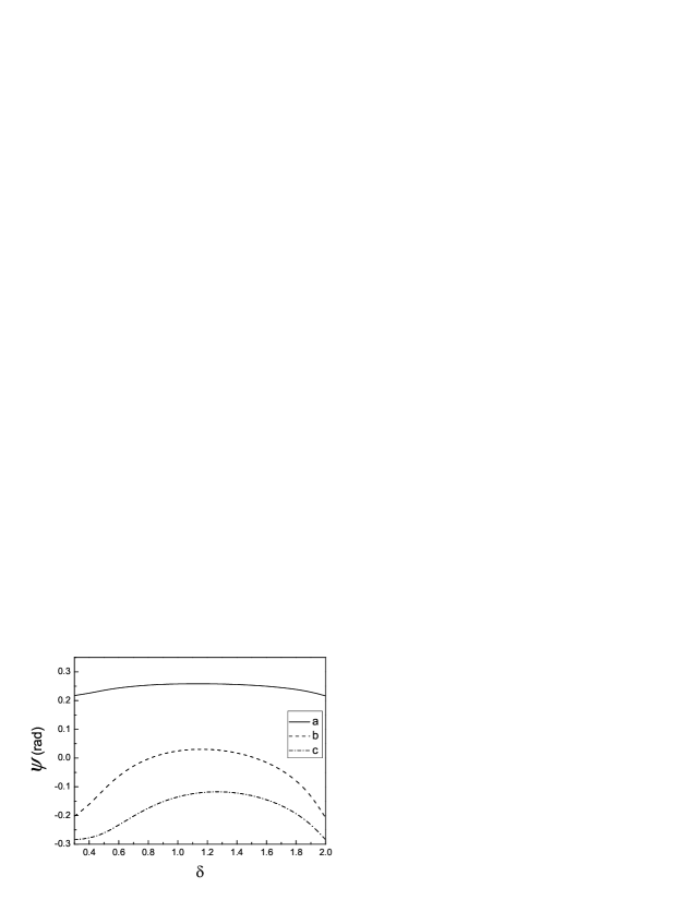
Figure 2: Optimal incident angel as a function of the power exponents $\delta$ for various effective frictions. The different parameters for each curve are (a) $\gamma_{12}=0.8$, $\gamma_{11}=1.8$, $\gamma_{22}=1.2$; (b) $\gamma_{12}=2.0$, $\gamma_{11}=2.5$, $\gamma_{22}=2.2$; (c) $\gamma_{12}=4.0$, $\gamma_{11}=4.8$, $\gamma_{22}=4.2$, others are the same as those used in Fig. 1.

Figure 3: Schematic illustration of the optimal incident angel for various power exponents $\delta$. The different parameters for each group of curves are (a) $\gamma_{12}=0.8$, $\gamma_{11}=1.8$, $\gamma_{22}=1.2$ for straight lines; and (b) $\gamma_{12}=4.0$, $\gamma_{11}=4.8$, $\gamma_{22}=4.2$ for dashed lines, other parameters are the same as those used in Fig. 1.

III non-Ohmic Anomalous transmission coefficient

In this section we evaluate the rate of a particle escape from the 2D metastable potential. Since difficulty makes it impossible to solve the Fokker-Planck equation with non-Ohmic friction, we use the method of reactive flux to derive the rate constant from Langevin dynamics. In the spirit of reactive flux calculation, particles are set evolving from the top of the barrier and the thermal rate constant is got from the ensemble average of trajectories starting with identical initial conditions but experience different stochastic histories. For a 2D system, the rate for a particle of unit mass 2Drate is defined as

$$k(t)=\frac{1}{Qh}\int d\vec{p}ds(\vec{p}\cdot\vec{n}_{s})\chi(\vec{p},\vec{q}_{s})e^{-H(\vec{p},\vec{q}_{s})/k_{{}_{B}}T}.$$ (10)

Where $\vec{p}$ is the momentum vector and $Q$ is the partition function for reactants integrating over the distribution of the ground states. $\chi(\vec{p},\vec{q}_{s})$, namely the characteristic function is a number which is equal to 1 for reactive trajectories ($\vec{p}\cdot\vec{n}_{s}>0$) and 0 for nonreactive ones ($\vec{p}\cdot\vec{n}_{s}<0$). Because of the stochastic nature of the dynamics, it is necessary to take into account all the different possible realizations of a trajectory. To do so $\chi(\vec{p},\vec{q}_{s})$ should be replaced by its non-equilibrium average $\chi(x_{{}_{10}},x_{{}_{20}},v_{{}_{10}},v_{{}_{20}})$ which results in a weighted factor with its value ranging from 0 to 1. The rate is then proportional to the total flux from reactants to products independent of the choice of dividing surface between reactants and products excluding the influence of the recrossing effects.

If the initial conditions are assumed to be at the top of the barrier, the rate constant corresponds to an ensemble of particles starting from ($x_{{}_{10}}=0,x_{{}_{20}},v_{{}_{10}},v_{{}_{20}}$) at $t=0$ and obeys the equilibrium distribution. Mathematically,

$$k(t) = \frac{1}{Qh}\prod^{2}_{i=1}\int^{\infty}_{-\infty}dx_{{}_{i0}}dv_{{}_{i0}}v_{{}_{10}}e^{-H(x_{{}_{10}},x_{{}_{20}},v_{{}_{10}},v_{{}_{20}})/k_{{}_{B}}T}\delta(x_{{}_{10}})\chi(x_{{}_{10}},x_{{}_{20}},v_{{}_{10}},v_{{}_{20}};t)$$ (11)

$$= \frac{e^{-V_{{}_{B}}/k_{B}T}}{Qh}\prod^{2}_{i=1}\int^{\infty}_{-\infty}dx_{{}_{i0}}dv_{{}_{i0}}v_{{}_{10}}e^{-\left[m_{ij}v_{{}_{i0}}v_{{}_{j0}}+\omega_{22}x^{2}_{{}_{20}}\right]/2k_{{}_{B}}T}\chi(x_{{}_{10}}=0,x_{{}_{20}},v_{{}_{10}},v_{{}_{20}};t),$$

with the system Hamiltonian $H(x_{{}_{10}},x_{{}_{20}},v_{{}_{10}},v_{{}_{20}})=\frac{1}{2}m_{ij}v_{{}_{i0}}v_{{}_{j0}}+\frac{1}{2}\omega_{ij}x_{{}_{i0}}x_{{}_{j0}}+V_{{}_{B}}$, and an initial Boltzmann form stationary probability distribution with a weight $k_{B}T$ at the metastable well is assumed when the temperature is much less than the barrier height of the metastable potential.

The total rate thus can be viewed as a transition state theory (TST) rate $k^{TST}=\frac{1}{Qh}e^{-V_{{}_{B}}/k_{B}T}$ TST1 ; TST2 ; TST3 multiplied by a factor $\kappa(t)$ between 0 and 1, namely the transmission coefficient, as we have got here

$$\kappa(t)=\left[1+\frac{\textrm{det}m_{ij}}{m_{22}}\left(\frac{C^{2}_{2}(t)}{\omega_{22}}-\frac{2m_{12}}{\textrm{det}m_{ij}}C_{3}(t)C_{4}(t)+\frac{m_{11}C^{2}_{4}(t)}{\textrm{det}m_{ij}}+\frac{\sigma^{2}_{x_{1}}(t)}{k_{B}T}\right)\right]^{-\frac{1}{2}}.$$ (12)

which describes the probability of a particle successfully escaped from the metastable well to recross the barrier. This expression for the fractional reactive index leads immediately to Kramers formula for the rate constant.

In order to individually inspect the dynamical corrections of $\kappa(t)$ to the TST rate, Fig. 4 gives the transient expression of it for various strength of system friction. Apparently seen from it, the value of $\kappa(t)$ keeps $1.0$ when $t=0$, showing no barrier recrossing behavior at the beginning. But as $t\rightarrow\infty$, $\kappa(t)$ stabilizes to a invariable constant between 0 and 1, namely the stationary transmission coefficient $\kappa_{\textrm{st}}$, representing the probability of a particle already escaped from the metastable potential well to recross the barrier. Mathematically, it creates a cutoff factor to the TST rate.

Meanwhile, by investigating the stationary transmission coefficient at various strength of system friction we can find: in most cases of non-Ohmic damping, $\kappa(t)$ stabilizes to a smaller $\kappa_{\textrm{st}}$ than the Ohmic case ($\delta=1.0$) except for some special one such as $\delta=1.2$. This implies the barrier recrossing of non-Ohmic system is generally stronger than the Ohmic case. The long memory aspect of friction is most possible to be at the origin of this behavior.

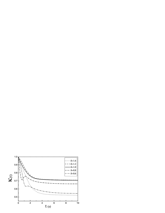
Figure 4: Transient expression of $\kappa(t)$ for various strength of system friction. Identical parameters are used as in Fig. 1.

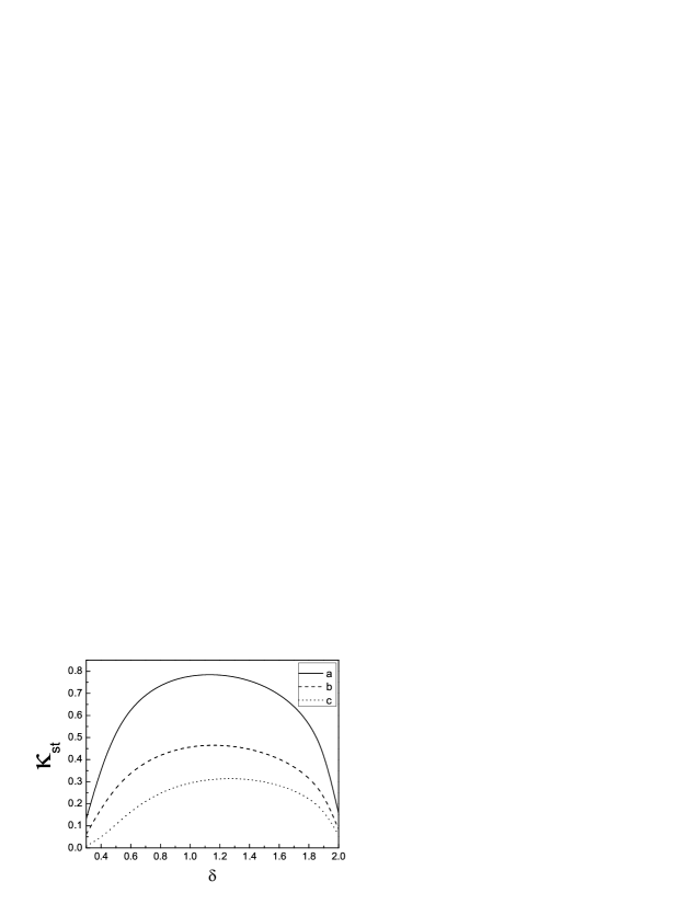
Figure 5: Stationary transmission coefficient $\kappa_{\textrm{st}}$ as a function of $\delta$ for various system frictions. Parameters used are identical to those in Fig 2.

For further understanding of this subject, the stationary transmission coefficient $\kappa_{\textrm{st}}$ is plotted in Fig. 5 as a function of $\delta$ for various system frictions. Again it is found to change non-monotonically with $\delta$. This is because, the friction of non-Ohmic system has a long memory in time. If the friction strength is weak (i.e. $\delta\rightarrow 0$), the motion of a particle depending greatly on the initial conditions. In the opposite aspect, strong friction strength (i.e. $\delta\rightarrow 2.0$) causes great viscous force to the particle. In both cases, it is unfavorable for the particle to pass the saddle point of the PES. This results in a smaller passing probability and a transmission coefficient than the normally Ohmic case.

Furthermore, comparing with the results of 1D non-Ohmic systemsJCP-Bao ; jlz , the 2D non-Ohmic system is found to have a bigger stationary transmission coefficient in the long time limit which means a weaker barrier recrossing effect. Particle diffusing in the 2D PES under non-Ohmic friction seldom returns after passing the saddle point of the potential. Macroscopically it results in a big net flux rate.

IV SUMMARY

In conclusion, a two-dimensional barrier passage has been investigated, where the particle is subjected to a non-Ohmic memory friction with power exponent $\delta$. The time-dependent passing probability and transmission coefficient are analytically obtained by using of the reaction flux method in a Langevin dynamic picture. In the long time limit, the passing probability, the optimal incident angle of the particle and the anomalous transmission coefficient are all found to be non-monotonic functions of the power exponent of the friction $\delta$. The long memory aspect of friction is most possible to be at the origin of this behavior. The relatively bigger stationary transmission coefficient reveals that there is less barrier recrossing in the two-dimensional system than the one-dimensional case. It is very difficult for the particle diffusing in the 2D PES under non-Ohmic friction to return after passing the saddle point of the potential. Thus results in a big net flux rate.

APPENDIX. THE EXPRESSIONS OF $\langle x_{1}(t)\rangle$

The quantities appear in the expression of $\langle x_{1}(t)\rangle$ are

$$\textsl{P}(s) = (m_{11}\hat{\beta}_{22}[s]+m_{22}\hat{\beta}_{11}[s]-2m_{12}\hat{\beta}_{12}[s])s^{3}$$

$$+(\textrm{det}\hat{\beta}_{ij}[s]+m_{11}\omega_{22}+m_{22}\omega_{11}-2m_{12}\omega_{12})s^{2}$$

$$+(\hat{\beta}_{11}[s]\omega_{22}+\hat{\beta}_{22}[s]\omega_{11}-2\hat{\beta}_{12}[s]\omega_{12})s$$

$$+(\textrm{det}m_{ij})s^{4}+\textrm{det}\omega_{ij},$$

$$\textsl{F}_{1}(s) = (m_{11}\hat{\beta}_{22}[s]+m_{22}\hat{\beta}_{11}[s]-2m_{12}\hat{\beta}_{12}[s])s^{2}$$

$$+(\textrm{det}\hat{\beta}_{ij}[s]+m_{11}\omega_{22}-m_{12}\omega_{12})s+(\textrm{det}m_{ij})s^{3}$$

$$+\hat{\beta}_{11}[s]\omega_{22}-\hat{\beta}_{12}[s]\omega_{12},$$

$$\textsl{F}_{2}(s) = (m_{12}\omega_{22}-m_{22}\omega_{12})s+\hat{\beta}_{12}[s]\omega_{22}-\hat{\beta}_{22}[s]\omega_{12},$$

$$\textsl{F}_{3}(s) = (\textrm{det}m_{ij})s^{2}+(m_{11}\hat{\beta}_{22}[s]-m_{12}\hat{\beta}_{12}[s])s$$

$$+m_{11}\omega_{22}-m_{12}\omega_{12},$$

$$\textsl{F}_{4}(s) = (m_{12}\hat{\beta}_{22}[s]-m_{22}\hat{\beta}_{12}[s])s+m_{12}\omega_{22}-m_{22}\omega_{12},$$

$$\textsl{F}_{5}(s) = m_{22}s^{2}+\hat{\beta}_{22}[s]s+\omega_{22},$$

$$\textsl{F}_{6}(s) = -m_{12}s^{2}-\hat{\beta}_{12}[s]s-\omega_{12}.$$

where $\hat{\beta}_{ij}[s]=\tilde{\gamma}_{ij}s^{\delta-1}$ is the Laplace transform of the friction kernel function and $\tilde{\gamma}_{ij}=\gamma_{ij}\omega_{r}^{1-\delta}\textrm{sin}^{-1}(\delta\pi/2)$ is namely the effective friction.

References

• (1) P. HΓ€nggi, P. Talkner, and M. Borkovec, Rev. Mod. Phys. 62, 251 (1990).
• (2) E. Pollak, J. Chem. Phys. 85, 865 (1986).
• (3) P. Talker, E. Pollak, and A. M. Berhkovskii, Chem. Phys. 235, 1 (1998).
• (4) T. Seideman and W. H. Miller, J. Chem. Phys. 95, 1768 (1991).
• (5) J. M. Sancho, A. H. Romero, and K. Lindenberg, J. Chem. Phys. 109, 9888 (1998).
• (6) E. Pollak and M. S. Child, J. Chem. Phys. 72, 1669 (1980).
• (7) W. Forst, Theory of Unimolecular Reaction (Academic, New York, 1973).
• (8) W. L. Hase, in Dynamics of Molecular Collisions, Part B, edited by W. H. Miller (Plenum, New York, 1976), p. 121.
• (9) A. B. Callear, in Modern Methods in Kinetics, Comprehensive Chemical Kinetics, Vol. 24, edited by C. H. Bamford and C. F. H. Tipper (Elsevier, New York, 1983) p.333.
• (10) H. A. Kramers, Physica (Utrecht) 7, 284 (1940).
• (11) L. Farkas, Z. Phys. Chem. 125, 236 (1927).
• (12) P. Talkner, Z. Phys. B 68, 201 (1987).
• (13) J. D. Bao, J. Chem. Phys. 124, 114103 (2006)
• (14) D. J. Tannor and D. Kohen, J. Chem. Phys. 100, 4932 (1994).
• (15) D. Kohen and D. J. Tannor, J. Chem. Phys. 103, 6013 (1995).
• (16) R. Metzler and J. Klafter, Phys. Rep. 339, 1 (2000).
• (17) J. D. Bao and Y. Z. Zhuo, Phys. Rev. Lett. 91, 138104 (2003).
• (18) Jing-Dong Bao, Yi-Zhong Zhuo. Phys. Rev. C 67, 064606 (2003).
• (19) U. Weiss, Quantum Dissipative Systems, 2nd ed. (World Scientific, Singapore, 1999).
• (20) N. Pottier, Physica A 317, 371 (2003).
• (21) H. Grabert, P. Schramm, and G.-L. Ingold, Phys. Rev. Lett. 58, 1285 (1987).
• (22) C. Y. Wang, Jia Y and J. D. Bao, Phys. Rev. C 77, 024603 (2008)
• (23) P. Pechukas, in Dynamics of Molecular Collisions, Part B, edited by W. H. Miller (Plenum, New York, 1976), p. 269.
• (24) J. L. Zhao and J. D. Bao, Phys. A 356, 517 (2005)