A spectral method for the wave equation of divergence-free vectors and symmetric tensors inside a sphere

Abstract

The wave equation for vectors and symmetric tensors in spherical coordinates is studied under the divergence-free constraint. We describe a numerical method, based on the spectral decomposition of vector/tensor components onto spherical harmonics, that allows for the evolution of only those scalar fields which correspond to the divergence-free degrees of freedom of the vector/tensor. The full vector/tensor field is recovered at each time-step from these two (in the vector case), or three (symmetric tensor case) scalar fields, through the solution of a first-order system of ordinary differential equations (ODE) for each spherical harmonic. The correspondence with the poloidal-toroidal decomposition is shown for the vector case. Numerical tests are presented using an explicit Chebyshev-tau method for the radial coordinate.

1 Introduction

Evolution partial differential equations (PDE) for vector fields under the divergence-free constraint appear in many physical models. Similar problems are to be solved with second-rank tensor fields. In most of these equations, if the initial data and boundary conditions satisfy the divergence-free condition, then the solution on a given time interval is divergence-free too. But from the numerical point of view, things can be more complicated and round-off errors can create undesired solutions, which may then trigger growing unphysical modes. Therefore, in the case of vector fields, several methods for the numerical solution of such PDEs have been devised, such as the constraint transport method [12] or the toroidal-poloidal decomposition [11, 20]. The aim of this paper is to present a new method for the case of symmetric tensor fields, which appear in general relativity within the so-called 3+1 approach [1], keeping in mind the vector case for which the method can be closely related to the toroidal-poloidal approach. We first give motivations for the numerical study of divergence-free vectors and tensors in Secs. 1.1 and 1.2; we briefly introduce our notations and conventions for spherical coordinates and grid in Sec. 1.3. The case of the vector divergence-free evolution is studied in Sec. 2, and the link with the poloidal-toroidal decomposition is detailed in Sec. 2.3. We then turn to the symmetric tensor case in Sec. 3 with the particular traceless condition in Sec. 3.3. A discussion of the treatment of boundary conditions is given in Sec. 4, with the particular point of inner boundary conditions (Sec. 4.3). Finally, some numerical experiments are reported in Sec. 5 to support our algorithms and concluding remarks are given in Sec. 6.

1.1 Divergence-free vector fields in relativistic magneto-hydrodynamics

In classical electrodynamics, the magnetic field is known to be divergence-free since Maxwell’s equations. This result can be extended to general relativistic electrodynamics as well. In classical hydrodynamics, the continuity equation can be expressed as $\partial_{t}\rho+\nabla\cdot(\rho\mathbf{u})=0$, where $\rho$ is the mass density of the fluid, and $\mathbf{u}$ its velocity. Various approximations give rise to divergence-free vectors. Incompressible fluids have constant density along flow lines and therefore verify that their velocity field $\mathbf{u}$ is divergence-free. Water is probably the most common example of an incompressible fluid. In an astrophysical context, the incompressible approximation can lead to a pretty good approximation of the behavior of compressible fluid provided that the flow’s Mach number is much smaller than unity. Another useful hydrodynamic approximation is the anelastic approximation, which essentially consists in filtering out the sound waves, whose extremely short time scale would otherwise force the use of an impractically small time step for numerical purposes. In general-relativistic magneto-hydrodynamics, the anelastic approximation takes the form $\nabla\cdot(\rho\Gamma\mathbf{u})=0$, where $\mathbf{u}$ is the coordinate fluid velocity, $\Gamma$ the Lorentz factor of the fluid, and $\rho$ its rest-mass density.

Divergence-free vectors have given rise to a large literature in numerical simulations. For example, while using an induction equation to numerically evolve a magnetic field, there is no guarantee that the divergence of the updated magnetic field is numerically conserved. The most common methods to conserve divergences in hyperbolic systems are constrained transport methods, projection methods or hyperbolic divergence cleaning methods (see [25] for a review).

1.2 Divergence-free symmetric tensors in general relativity

The basic formalism of general relativity uses four-dimensional objects and, in particular, symmetric four-tensors as the metric or the stress-energy tensor. A choice of the gauge, which comes naturally to describe the propagation of gravitational waves is the harmonic gauge (e.g. [8]), for which the divergence of the four-metric is zero. The 3+1 formalism (see [1] for a review) is an approach to general relativity introducing a slicing of the four-dimensional spacetime by three-dimensional spacelike surfaces, which have a Riemannian induced three-metric. With this formalism, the four-dimensional tensors of general relativity are projected onto these three-surfaces as three-dimensional tensors. Consequently, the choice of the gauge on the three-surface is a major issue for the computation of the solutions of Einstein’s equations.

The divergence-free condition on the conformal three-metric has already been put forward by Dirac [9] in Cartesian coordinates, and generalized to any type of coordinates in [4]. This conformal three-metric obeys an evolution equation which can be cast into a wave-like propagation equation. Far from any strong source of gravitational field, this evolution equation tends to a tensor wave equation, under the gauge constraint. With the choice of the generalized Dirac gauge this translates into the system we study in Sec. 3, with the addition of one extra constraint: the fact that the determinant of the conformal metric must be one (Eq. (167) of [4]).

The choice of spherical coordinates and components comes naturally with the study of isolated spheroidal objects as relativistic stars or black holes. Moreover, boundary conditions for the metric or for the hydrodynamics equations can be better expressed and implemented using tensor or vector components in the spherical basis. The numerical simulations of astrophysically relevant objects in general relativity must therefore be able to deal with the evolution of divergence-free symmetric tensors, in spherical coordinates and components. A particular care must be given to the fulfillment of the divergence-free condition, since this additional constraint sets the spatial gauge on the spacetime.

1.3 Spherical components and coordinates

In the following, unless specified, all the vector and tensor fields shall be functions of the four spacetime coordinates $\mathbf{V}(t,r,\theta,\varphi)$ and $\mathbf{h}(t,r,\theta,\varphi)$, where $(r,\theta,\varphi)$ are the polar spherical coordinates. The associated spherical orthonormal basis is defined as:

$$\mathbf{e}_{r}=\frac{\partial}{\partial r},\ \mathbf{e}_{\theta}=\frac{1}{r}\frac{\partial}{\partial\theta},\ \mathbf{e}_{\varphi}=\frac{1}{r\sin\theta}\frac{\partial}{\partial\varphi}.$$ (1)

The vector and symmetric tensor fields shall be described by their contravariant components $\left\{V^{r},V^{\theta},V^{\varphi}\right\}$ and $\left\{h^{rr},h^{r\theta},h^{r\varphi},h^{\theta\theta},h^{\theta\varphi},h^{\varphi\varphi}\right\}$, using this spherical basis:

$$\mathbf{V}=\sum_{i=r,\theta,\varphi}V^{i}\,\mathbf{e}_{i},\quad\mathbf{h}=\sum_{i=r,\theta,\varphi}\sum_{j=r,\theta,\varphi}h^{ij}\,\mathbf{e}_{i}\otimes\mathbf{e}_{j}.$$ (2)

The scalar Laplace operator acting on a field $\phi(r,\theta,\varphi)$ is written:

$$\Delta\phi=\frac{\partial^{2}\phi}{\partial r^{2}}+\frac{2}{r}\frac{\partial\phi}{\partial r}+\frac{1}{r^{2}}\Delta_{\theta\varphi}\phi,$$ (3)

where $\Delta_{\theta\varphi}$ is the angular part of the Laplace operator, containing only derivatives with respect to $\theta$ or $\varphi$:

$$\Delta_{\theta\varphi}\phi=\frac{\partial^{2}\phi}{\partial\theta^{2}}+\frac{\cos\theta}{\sin\theta}\frac{\partial\phi}{\partial\theta}+\frac{1}{\sin^{2}\theta}\frac{\partial^{2}\phi}{\partial\varphi^{2}}.$$ (4)

We now introduce scalar spherical harmonics, defined on the sphere as (see Sec. 18.11 of [2] for more details)

$$\forall\ell\geq 0,\ \forall m,\ 0\leq m\leq\ell,\quad Y_{\ell}^{m}(\theta,\varphi)=e^{im\varphi}P_{\ell}^{m}(\cos\theta),$$ (5)

where $P_{\ell}^{m}$ is the associated Legendre function. For negative $m$, spherical harmonics are defined

$$\forall m,\ -\ell\leq m<0,\quad Y_{\ell}^{m}(\theta,\varphi)=(-1)^{m}e^{im\varphi}P_{\ell}^{|m|}(\cos\theta).$$ (6)

Their two main properties used in this study are that they form a complete basis for the development of regular scalar functions on the sphere, and that they are eigenfunctions of the angular Laplace operator:

$$\forall(\ell,m),\ \Delta_{\theta\varphi}Y_{\ell}^{m}=-\ell(\ell+1)Y_{\ell}^{m}.$$ (7)

2 Vector case

We look for the solution of the following initial-boundary value problem of unknown vector $\mathbf{V}$, inside a sphere of (constant) radius $R$, thus $\forall(\theta,\varphi)$:

$$\forall t\geq 0,\ \forall r<R,\qquad \frac{\partial^{2}\mathbf{V}}{\partial t^{2}}=\mathbf{\Delta V},$$ (8)

$$\forall t\geq 0,\ \forall r\leq R,\qquad \mathbf{\nabla}\cdot\mathbf{V}=0,$$ (9)

$$\forall r\leq R,\qquad \mathbf{V}(0,r,\theta,\varphi)=\mathbf{v}_{0}(r,\theta,\varphi),$$

$$\forall r\leq R,\qquad \left.\frac{\partial\mathbf{V}}{\partial t}\right|_{t=0}=\mathbf{w}_{0}(r,\theta,\varphi),$$

$$\forall t\geq 0,\qquad \mathbf{V}(t,R,\theta,\varphi)=\mathbf{b}_{0}(t,\theta,\varphi).$$ (10)

$\mathbf{v}_{0},\mathbf{w}_{0}$ and $\mathbf{b}_{0}$ are given regular functions for initial data and boundary conditions, respectively. $\mathbf{\Delta}$ is the vector Laplace operator, which in spherical coordinates and in the contravariant representation (2) using the orthonormal basis (1) reads:

$$\left(\mathbf{\Delta V}\right)^{r}={} \frac{\partial^{2}V^{r}}{\partial r^{2}}+\frac{4}{r}\frac{\partial V^{r}}{\partial r}+\frac{2V^{r}}{r^{2}}+\frac{1}{r^{2}}\Delta_{\theta\varphi}V^{r}-\frac{2}{r}\Theta,$$ (11)

$$\left(\mathbf{\Delta V}\right)^{\theta}={} \frac{\partial^{2}V^{\theta}}{\partial r^{2}}+\frac{2}{r}\frac{\partial V^{\theta}}{\partial r}+\frac{1}{r^{2}}\left(\Delta_{\theta\varphi}V^{\theta}+2\frac{\partial V^{r}}{\partial\theta}-\frac{V^{\theta}}{\sin^{2}\theta}-2\frac{\cos\theta}{\sin^{2}\theta}\frac{\partial V^{\varphi}}{\partial\varphi}\right),$$

$$\left(\mathbf{\Delta V}\right)^{\varphi}={} \frac{\partial^{2}V^{\varphi}}{\partial r^{2}}+\frac{2}{r}\frac{\partial V^{\varphi}}{\partial r}+\frac{1}{r^{2}}\left(\Delta_{\theta\varphi}V^{\varphi}+\frac{2}{\sin\theta}\frac{\partial V^{r}}{\partial\varphi}+2\frac{\cos\theta}{\sin^{2}\theta}\frac{\partial V^{\theta}}{\partial\varphi}-\frac{V^{\varphi}}{\sin^{2}\theta}\right),$$

with the divergence $\Theta$

$$\Theta\equiv\mathbf{\nabla}\cdot\mathbf{V}=\frac{\partial V^{r}}{\partial r}+\frac{2V^{r}}{r}+\frac{1}{r}\left(\frac{\partial V^{\theta}}{\partial\theta}+\frac{V^{\theta}}{\tan\theta}+\frac{1}{\sin\theta}\frac{\partial V^{\varphi}}{\partial\varphi}\right).$$ (12)

One can remark that a necessary condition for this system to be well-posed is that

$$\mathbf{\nabla}\cdot\mathbf{v}_{0}=\mathbf{\nabla}\cdot\mathbf{w}_{0}=0.$$ (13)

In addition, the boundary setting at $r=R$ is actually overdetermined: the three conditions are not independent because of the divergence constraint. This aspect of the problem will be developed in more details in Sec. 4.1.

In the rest of this Section, we devise a method to verify both equations (8) and (9). This technique is similar to that presented in [3] with the difference that we motivate it by the use of vector spherical harmonics, and can easily be related to the poloidal-toroidal decomposition method, as discussed in Sec. 2.3.

2.1 Decomposition on vector spherical harmonics

The first step is to decompose the angular dependence of the vector field $\mathbf{V}$ onto a basis of pure spin vector harmonics (see [24] for a review):

$$\mathbf{V}(t,r,\theta,\varphi)=\sum_{\ell,m}\left(E^{\ell m}(t,r)\mathbf{Y}^{E}_{\ell m}+B^{\ell m}(t,r)\mathbf{Y}^{B}_{\ell m}+R^{\ell m}(t,r)\mathbf{Y}^{R}_{\ell m}\right),$$ (14)

defined from the scalar spherical harmonics as

$$\forall\ell>0,\ \forall-\ell\leq m\leq\ell,\ \mathbf{Y}^{E}_{\ell m}={} r\ \nabla Y_{\ell}^{m},$$ (15)

$$\forall\ell>0,\ \forall-\ell\leq m\leq\ell,\ \mathbf{Y}^{B}_{\ell m}={} \mathbf{e}_{r}\times\mathbf{Y}^{E}_{\ell m},$$ (16)

$$\forall\ell\geq 0,\ \forall-\ell\leq m\leq\ell,\ \mathbf{Y}^{R}_{\ell m}={} Y_{\ell}^{m}\ \mathbf{e}_{r};$$ (17)

where $\nabla$ is the gradient in the orthonormal basis (1). Note that both $\mathbf{Y}^{E}_{\ell m}$ and $\mathbf{Y}^{B}_{\ell m}$ are purely transverse, whereas $\mathbf{Y}^{R}_{\ell m}$ is purely radial. From this decomposition, we define the pure spin components of $\mathbf{V}$ by summing all the multipoles with scalar spherical harmonics (5):

$$V^{\eta}(t,r,\theta,\varphi)={} \sum_{\ell,m}E^{\ell m}\,Y_{\ell}^{m},$$ (18)

$$V^{\mu}(t,r,\theta,\varphi)={} \sum_{\ell,m}B^{\ell m}\,Y_{\ell}^{m},$$ (19)

the last one being the usual $r$-component

$$\sum_{\ell,m}R^{\ell m}\,Y_{\ell}^{m}=V^{r}.$$ (20)

The advantages of these pure spin components are first, that by construction they can be expanded onto the scalar spherical harmonic basis, and second, that angular derivatives appearing in all equations considered transform into the angular Laplace operator (7).

To be more explicit, $(V^{\eta},V^{\mu})$ can be related to the vector spherical components by (see also [4]):

$$V^{\theta}=\frac{\partial V^{\eta}}{\partial\theta}-\frac{1}{\sin\theta}\frac{\partial V^{\mu}}{\partial\varphi},$$ (21)

$$V^{\varphi}=\frac{1}{\sin\theta}\frac{\partial V^{\eta}}{\partial\varphi}+\frac{\partial V^{\mu}}{\partial\theta};$$

and inversely

$$\Delta_{\theta\varphi}V^{\eta}=\frac{\partial V^{\theta}}{\partial\theta}+\frac{V^{\theta}}{\tan\theta}+\frac{1}{\sin\theta}\frac{\partial V^{\varphi}}{\partial\varphi},$$ (22)

$$\Delta_{\theta\varphi}V^{\mu}=\frac{\partial V^{\varphi}}{\partial\theta}+\frac{V^{\varphi}}{\tan\theta}-\frac{1}{\sin\theta}\frac{\partial V^{\theta}}{\partial\varphi}.$$ (23)

Let us here point out that the angular Laplace operator $\Delta_{\theta\varphi}$ is diagonal with respect to the functional basis of spherical harmonics and, therefore, the above relations can directly be used to obtain $V^{\eta}$ and $V^{\mu}$.

Thus, if the fields are defined on the whole sphere $\theta\in[0,\pi],\ \varphi\in[0,2\pi)$, it is possible to transform the usual components $\left(V^{\theta},V^{\varphi}\right)$ to the pure spin ones $\left(V^{\eta},V^{\mu}\right)$ by this one-to-one transformation, up to a constant ($\ell=0$ part) for $V^{\eta}$ and $V^{\mu}$. Since this constant is not relevant, it shall be set to zero and disregarded in the following. Therefore, a vector field shall be represented equivalently by its usual spherical components or by $\left(V^{r},V^{\eta},V^{\mu}\right)$.

2.2 Divergence-free degrees of freedom

From the vector spherical harmonic decomposition, we now compute two scalar fields that represent the divergence-free degrees of freedom of a vector. We start from the divergence of a general vector $\mathbf{W}$, expressed in terms of pure spin components:

$$\Theta=\frac{\partial W^{r}}{\partial r}+2\frac{W^{r}}{r}+\frac{1}{r}\Delta_{\theta\varphi}W^{\eta};$$ (24)

where $W^{\eta}$ has been computed for the vector $\mathbf{W}$ from Eq. (22). This shows that the divergence of $\mathbf{W}$ does not depend on the pure spin component $W^{\mu}$. On the other hand, it is well-known that any sufficiently smooth and rapidly decaying vector field $\mathbf{W}$ can be (uniquely on $\mathbb{R}^{3}$) decomposed as a sum of a gradient and a divergence-free part (Helmholtz’s theorem)

$$\mathbf{W}=\nabla\phi+\mathbf{D}_{0},$$ (25)

with $\nabla\cdot\mathbf{D}_{0}=0$. From the formula (23), one can check that the component $W^{\mu}$ only depends on $\mathbf{D}_{0}$. Next, taking the curl of $\mathbf{W}$ and, in particular, combining the $\theta$- and $\varphi$- components of this curl, one has that $\partial_{r}W^{\eta}+\frac{W^{\eta}}{r}-\frac{W^{r}}{r}$ has the same property of being invariant under the addition of any gradient field to $\mathbf{W}$, thus depends only on $\mathbf{D}_{0}$. Therefore, we define the potential

$$A=\frac{\partial W^{\eta}}{\partial r}+\frac{W^{\eta}}{r}-\frac{W^{r}}{r}.$$ (26)

As a consequence, we have that

$$\mathbf{D}_{0}=0\iff W^{\mu}=0\textrm{ and }A=0.$$ (27)

We have thus identified two scalar degrees of freedom for a divergence-free vector field, which can be easily related to the well-known poloidal-toroidal decomposition (Sec. 2.3), but have the advantage of being generalizable to the symmetric tensor case.

We now write the wave equation (8) in terms of $V^{\mu}$ and $A$ (computed from $V^{r}$ and $V^{\eta}$). It is first interesting to examine the pure spin components of the vector Laplace operator (11):

$$\left(\mathbf{\Delta V}\right)^{\eta}={} \Delta V^{\eta}+2\frac{V^{r}}{r^{2}},$$ (28)

$$\left(\mathbf{\Delta V}\right)^{\mu}={} \Delta V^{\mu};$$ (29)

one sees that the equation for $V^{\mu}$ decouples from the system, therefore Eq. (8) implies that

$$\frac{\partial^{2}V^{\mu}}{\partial t^{2}}=\Delta V^{\mu}.$$ (30)

Forming then from (11) and (28) an equation for the potential $A$, which is a consequence of the original wave equation (8), we obtain

$$\frac{\partial^{2}A}{\partial t^{2}}=\Delta A.$$ (31)

We are left with two scalar wave equations, (30) and (31), for the divergence-free part of the vector field $\mathbf{V}$. The recovery of the full vector field shall be discussed in Sec. 2.4; the treatment of boundary conditions shall be presented in Sec. 4.1.

2.3 Link with poloidal-toroidal decomposition

According to the classical poloidal-toroidal decomposition, a divergence-free vector field $\mathbf{F}$ can be considered to be generated by two scalar potentials $\Phi$ and $\Psi$, via

$$\mathbf{F}=\mathbf{\nabla}\times(\Psi\mathbf{k})+\nabla\times\nabla\times(\Phi\mathbf{k})$$ (32)

Here, $\mathbf{k}$ is a unit vector, called the pilot vector, which is chosen according to the geometry of the problem considered. In [6, 7], $\mathbf{k}$ is chosen to be $\mathbf{e}_{z}$ in cylindrical coordinates. One can also find the decomposition $\mathbf{F}=\mathbf{\nabla}\times(A(r,\theta)\mathbf{e_{\varphi}})+B(r,\theta)\mathbf{e_{\varphi}}$ when considering axisymmetric solenoidal fields (see for example [17]). The latter representation makes $A$ appear clearly as a poloidal component, and $B$ as a toroidal component. In order to link the general poloidal-toroidal formalism to our previous potentials, we chose $\mathbf{k}=\mathbf{e}_{r}$ in spherical coordinates (sometimes called the Mie decomposition, see [10] ). Then, one can show that

$$\mathbf{F}=-\frac{1}{r^{2}}\Delta_{\theta\varphi}\Phi\,\mathbf{e}_{r}+\frac{1}{r}\left(\frac{1}{\sin\theta}\partial_{\varphi}\Psi+\partial_{\theta}\partial_{r}\Phi\right)\mathbf{e}_{\theta}+\frac{1}{r}\left(-\partial_{\theta}\Psi+\frac{1}{\sin\theta}\partial_{\varphi}\partial_{r}\Phi\right)\mathbf{e}_{\varphi}$$ (33)

Hence, we can identify the former pure spin components $F^{\eta}$ and $F^{\mu}$ through

$$F^{\eta}=\frac{1}{r}\partial_{r}\Phi$$

$$F^{\mu}=-\frac{1}{r}\Psi$$

Therefore, the potential $A$ is linked to the potential $\Phi$ via

$$A=\frac{1}{r}\partial_{r}^{2}\Phi+\frac{1}{r^{3}}\Delta_{\theta\varphi}\Phi=\Delta\left(\frac{\Phi}{r}\right)$$ (34)

which gives us a compatibility condition

$$\Delta_{\theta\varphi}A=-\Delta(rF^{r})$$ (35)

The latter equation expresses that $\partial_{r}(r^{2}\Theta)=0$ for the original vector. Since our vector is a regular function of coordinates, it expresses that $\Theta=0$.

One can also show the following relations

$$\mathbf{e}_{r}\cdot\nabla\times\mathbf{F}=\frac{1}{r}\Delta_{\theta\varphi}F^{\mu}$$

$$\mathbf{e}_{r}\cdot\nabla\times\nabla\times\mathbf{F}=\frac{1}{r}\Delta_{\theta\varphi}A$$

2.4 Integration scheme

We defer to Sec. 5.1 the numerical details about the integration procedure, and we sketch here the various steps. From the result of Sec. 2.2, the problem (8)-(9) can be transformed into two initial-value boundary problems, for the component $V^{\mu}$ (30) and the potential $A$ (31) respectively. Initial data can be deduced from $\mathbf{v}_{0}$ and $\mathbf{w}_{0}$, so that $V^{\mu}(t=0)$ and $\partial V^{\mu}/\partial t(t=0)$ are the $\mu$-components of, respectively, $\mathbf{v}_{0}$ and $\mathbf{w}_{0}$. The same is true for the $A$ potential. The determination of boundary conditions from the knowledge of $\mathbf{b}_{0}$ shall be discussed in Sec. 4. We therefore assume here that we have computed the component $V^{\mu}$ and the potential $A$, inside the sphere of radius $R$, for a given interval $[0,T]$, and we show how to recover the whole vector $\mathbf{V}$.

The pure spin components $\left(V^{r},V^{\eta}\right)$ of the vector $\mathbf{V}$ are obtained by solving the system of PDEs composed by the definition of the potential $A$ (26), together with the divergence-free condition (24). From their definitions (18)-(20), it is clear that the angular parts of both $V^{r}$ and $V^{\eta}$ can be decomposed onto the basis of scalar spherical harmonics, and therefore $A$ as well:

$$A(t,r,\theta,\varphi)=\sum_{\ell,m}A^{\ell m}(t,r)Y_{\ell}^{m}(\theta,\varphi).$$ (36)

We are left with the following set of systems of ordinary differential equations in the $r$-coordinate:

$$\forall\ell>0,\,\forall m\ -\ell\leq m\leq\ell,\quad\left\{\begin{aligned} \frac{\partial R^{\ell m}}{\partial r}+2\frac{R^{\ell m}}{r}-\frac{\ell(\ell+1)}{r}E^{\ell m}={}&0\\ \frac{\partial E^{\ell m}}{\partial r}+\frac{E^{\ell m}}{r}-\frac{R^{\ell m}}{r}={}&A^{\ell m}\end{aligned}\right..$$ (37)

The potential $A$ being given, the pure spin components $V^{r}$ and $V^{\eta}$ are obtained from this system, with the boundary conditions discussed in Sec. 4.1. The $\mu$-component is already known too, so it is possible to compute the spherical components of $\mathbf{V}$ $\forall t\in[0,T]$, from Eqs. (21). Note that all angular derivatives present in this system (37) are only in the form of the angular Laplace operator $\Delta_{\theta\varphi}$ (4). It must also be emphasized that the divergence-free condition is not enforced in terms of spherical components (Eq. (12)), but in terms of pure spin components. Thus, if the value of the divergence is numerically checked, it shall be higher than machine precision, because of the numerical derivatives one must compute to pass from pure spin to spherical components (Eqs. (21)).

The properties of the system (37) are easy to study. Substituting $R^{\ell m}$ in the first line by its expression as a function of $E^{\ell m}$ and $A^{\ell m}$ (obtained from the second line), one gets a simple Poisson equation:

$$\Delta\left(rE^{\ell m}\right)=r\frac{\partial A^{\ell m}}{\partial r}+2A^{\ell m}.$$ (38)

The discussion about boundary conditions, homogeneous solutions and regularity for $r=0$ and $r\to\infty$ are immediately deduced from those of the Poisson equation (see e.g. [13]).

In the case where a source $\mathbf{S}$ is present on the right-hand side of the problem (8), the method of imposing $\nabla\cdot\mathbf{V}=0$ can be generalized by adding sources to Eqs. (30)-(31), which are deduced from $\mathbf{S}$. Indeed, it is easy to show that the source for the equation for $V^{\mu}$ is the pure spin $\mu$-component of $\mathbf{S}$ and the source for the equation for $A$ is the equivalent potential computed from $\mathbf{S}$ pure spin components, using formula (26). Note that an integrability condition for this problem is that the source be divergence-free too. Therefore, for a well-posed problem, any gradient term present in $\mathbf{S}$ can be considered as spurious and is naturally removed by this method, since the $\mu$-component and the $A$ potential are both insensitive to the gradient parts.

3 Symmetric tensor case

Similarly to the vector case studied in Sec. 2, we look here for the solution of an initial-boundary value problem of unknown symmetric tensor $\mathbf{h}$, inside a sphere of radius $R$. As explained in Sec. 1.3, the symmetric tensor $\mathbf{h}$ shall be represented by its contravariant components $h^{ij}(=h^{ji})$, where the indices run from $1(r)$ to $3(\varphi)$; moreover, we suppose that all components of $\mathbf{h}$ decay to zero at least as fast as $1/r$, as $r\to\infty$. We shall also use the Einstein summation convention over repeated indices.

Thus the problem is written, $\forall(\theta,\varphi)$:

$$\forall t\geq 0,\ \forall r<R,\qquad \frac{\partial^{2}h^{ij}}{\partial t^{2}}=\Delta h^{ij},$$ (39)

$$\forall t\geq 0,\ \forall r\leq R,\qquad \nabla_{j}h^{ij}=0,$$ (40)

$$\forall r\leq R,\qquad h^{ij}(0,r,\theta,\varphi)=\alpha^{ij}_{0}(r,\theta,\varphi),$$

$$\forall r\leq R,\qquad \left.\frac{\partial h^{ij}}{\partial t}\right|_{t=0}=\gamma^{ij}_{0}(r,\theta,\varphi),$$

$$\forall t\geq 0,\qquad h^{ij}(t,R,\theta,\varphi)=\beta^{ij}_{0}(t,\theta,\varphi).$$ (41)

The tensors $\alpha^{ij}_{0},\gamma^{ij}_{0}$ and $\beta^{ij}_{0}$ are given regular functions for initial data and boundary conditions, respectively. The full expression of the tensor Laplace operator in spherical coordinates and in the orthonormal spherical basis (1) is given by Eqs. (123)-(128) of [4] and shall not be recalled here. We point out again that the boundary setting at $r=R$ is overdetermined: this is discussed in more detail in Sec. 4.2.

We introduce the vector $\mathbf{H}$, defined as the divergence of $h^{ij}$ and given in the spherical contravariant components (2) by:

$$H^{i}\equiv\nabla_{j}h^{ij}\iff\left\{\begin{aligned} H^{r}={}&\frac{\partial h^{rr}}{\partial r}+\frac{2h^{rr}}{r}+\frac{1}{r}\left(\frac{\partial h^{r\theta}}{\partial\theta}+\frac{1}{\sin\theta}\frac{\partial h^{r\varphi}}{\partial\varphi}-h^{\theta\theta}-h^{\varphi\varphi}+\frac{h^{r\theta}}{\tan\theta}\right),\\ H^{\theta}={}&\frac{\partial h^{r\theta}}{\partial r}+\frac{3h^{r\theta}}{r}+\frac{1}{r}\left(\frac{\partial h^{\theta\theta}}{\partial\theta}+\frac{1}{\sin\theta}\frac{\partial h^{\theta\varphi}}{\partial\varphi}+\frac{1}{\tan\theta}\left(h^{\theta\theta}-h^{\varphi\varphi}\right)\right),\\ H^{\varphi}={}&\frac{\partial h^{r\varphi}}{\partial r}+\frac{3h^{r\varphi}}{r}+\frac{1}{r}\left(\frac{\partial h^{\theta\varphi}}{\partial\theta}+\frac{1}{\sin\theta}\frac{\partial h^{\varphi\varphi}}{\partial\varphi}+\frac{2h^{\theta\varphi}}{\tan\theta}\right)=0.\end{aligned}\right.$$ (42)

We now detail, in the rest of this Section, a method to verify both evolution equation (39) and the divergence-free constraint (40).

3.1 Decomposition on tensor spherical harmonics

As in the vector case (Sec. 2.1), we start by decomposing the angular dependence of the tensor field $h^{ij}$ onto pure spin tensor harmonics, introduced by [21] and [27] (we again use the notations of [24]):

$$\mathbf{h}(t,r,\theta,\varphi)=\sum_{\ell,m}\left(L_{0}^{\ell m}\mathbf{T}^{L_{0}}_{\ell m}+T_{0}^{\ell m}\mathbf{T}^{T_{0}}_{\ell m}+E_{1}^{\ell m}\mathbf{T}^{E_{1}}_{\ell m}+B_{1}^{\ell m}\mathbf{T}^{B_{1}}_{\ell m}+E_{2}^{\ell m}\mathbf{T}^{E_{2}}_{\ell m}+B_{2}^{\ell m}\mathbf{T}^{B_{2}}_{\ell m}\right),$$ (43)

where $\left(L_{0}^{\ell m},T_{0}^{\ell m},E_{1}^{\ell m},B_{1}^{\ell m},E_{2}^{\ell m},B_{2}^{\ell m}\right)$ are all functions of only $(t,r)$. Complete definitions and properties of this set of tensor harmonics can be found in [24]. Note that these harmonics have been devised in order to describe gravitational radiation, far from any source. In that respect, the most relevant harmonics are $\mathbf{T}^{E_{2}}$ and $\mathbf{T}^{B_{2}}$, since they are transverse and traceless. The pure spin components of the tensor $\mathbf{h}$ are defined as:

$$h^{rr}(t,r,\theta,\varphi)=\sum_{\ell,m}L_{0}^{\ell m}\,Y_{\ell}^{m},$$ (44)

$$h^{\tau}(t,r,\theta,\varphi)=\sum_{\ell,m}T_{0}^{\ell m}\,Y_{\ell}^{m},$$ (45)

$$h^{\eta}(t,r,\theta,\varphi)=\sum_{\ell,m}E_{1}^{\ell m}\,Y_{\ell}^{m},$$ (46)

$$h^{\mu}(t,r,\theta,\varphi)=\sum_{\ell,m}B_{1}^{\ell m}\,Y_{\ell}^{m},$$ (47)

$$h^{\mathcal{W}}(t,r,\theta,\varphi)=\sum_{\ell,m}E_{2}^{\ell m}\,Y_{\ell}^{m},$$ (48)

$$h^{\mathcal{X}}(t,r,\theta,\varphi)=\sum_{\ell,m}B_{2}^{\ell m}\,Y_{\ell}^{m}.$$ (49)

Explicit relations between the last five components and the usual spherical components (2) are now given.

$$h^{\tau}=h^{\theta\theta}+h^{\varphi\varphi}$$ (50)

is transverse; and the total trace is simply given by

$$h=h^{rr}+h^{\tau}.$$ (51)

In the following we shall use either the component $h^{\tau}$ or the trace. The components $h^{\eta}$ and $h^{\mu}$ have similar formulas to those of the vector pure spin components, as $\left\{h^{ri}\right\}_{i=1,2,3}$ can be seen as a vector:

$$h^{r\theta}=\frac{\partial h^{\eta}}{\partial\theta}-\frac{1}{\sin\theta}\frac{\partial h^{\mu}}{\partial\varphi},$$ (52)

$$h^{r\varphi}=\frac{1}{\sin\theta}\frac{\partial h^{\eta}}{\partial\varphi}+\frac{\partial h^{\mu}}{\partial\theta};$$

the reverse formula being similar to Eqs. (22) and (23), they are not recalled here. Finally, the last two components are obtained by:

$$P\equiv\frac{\left(h^{\theta\theta}-h^{\varphi\varphi}\right)}{2}={} \frac{\partial^{2}h^{\mathcal{W}}}{\partial\theta^{2}}-\frac{1}{\tan\theta}\frac{\partial h^{\mathcal{W}}}{\partial\theta}-\frac{1}{\sin^{2}\theta}\frac{\partial^{2}h^{\mathcal{W}}}{\partial\varphi^{2}}-2\frac{\partial}{\partial\theta}\left(\frac{1}{\sin\theta}\frac{\partial h^{\mathcal{X}}}{\partial\varphi}\right),$$ (53)

$$h^{\theta\varphi}={} \frac{\partial^{2}h^{\mathcal{X}}}{\partial\theta^{2}}-\frac{1}{\tan\theta}\frac{\partial h^{\mathcal{X}}}{\partial\theta}-\frac{1}{\sin^{2}\theta}\frac{\partial^{2}h^{\mathcal{X}}}{\partial\varphi^{2}}+2\frac{\partial}{\partial\theta}\left(\frac{1}{\sin\theta}\frac{\partial h^{\mathcal{W}}}{\partial\varphi}\right);$$

and the inverse relations are given by:

$$\Delta_{\theta\varphi}\left(\Delta_{\theta\varphi}+2\right)h^{\mathcal{W}}={} \frac{\partial^{2}P}{\partial\theta^{2}}+\frac{3}{\tan\theta}\frac{\partial P}{\partial\theta}-\frac{1}{\sin^{2}\theta}\frac{\partial^{2}P}{\partial\varphi^{2}}-2P+\frac{2}{\sin\theta}\frac{\partial}{\partial\varphi}\left(\frac{\partial h^{\theta\varphi}}{\partial\theta}+\frac{h^{\theta\varphi}}{\tan\theta}\right),$$ (54)

$$\Delta_{\theta\varphi}\left(\Delta_{\theta\varphi}+2\right)h^{\mathcal{X}}={} \frac{\partial^{2}h^{\theta\varphi}}{\partial\theta^{2}}+\frac{3}{\tan\theta}\frac{\partial h^{\theta\varphi}}{\partial\theta}-\frac{1}{\sin^{2}\theta}\frac{\partial^{2}h^{\theta\varphi}}{\partial\varphi^{2}}-2h^{\theta\varphi}-\frac{2}{\sin\theta}\frac{\partial}{\partial\varphi}\left(\frac{\partial P}{\partial\theta}+\frac{P}{\tan\theta}\right).$$ (55)

Here as for the vector case, the $h^{\eta}$ and $h^{\mu}$ components do not contain any relevant $\ell=0$ term, whereas $h^{\mathcal{W}}$ and $h^{\mathcal{X}}$ contain neither $\ell=0$, nor $\ell=1$ terms, as expected for transverse traceless parts of the tensor $\mathbf{h}$. We shall use any set of components of the tensor $\mathbf{h}$: either the usual ones $\left\{h^{ij}\right\}$, using the spherical basis, or the pure spin ones $\left\{h^{rr},h^{\tau}\textrm{(or }h\textrm{)},h^{\eta},h^{\mu},h^{\mathcal{W}},h^{\mathcal{X}}\right\}$.

3.2 Divergence-free degrees of freedom

The vector $\mathbf{H}$ defined as the divergence of $\mathbf{h}$ in Eq. (42) can be expanded in terms of vector pure spin components, which are then written as functions of the tensor pure spin components of $\mathbf{h}$ (we use the trace $h$ instead of $h^{\tau}$):

$$H^{r}={} \frac{\partial h^{rr}}{\partial r}+\frac{3h^{rr}}{r}+\frac{1}{r}\left(\Delta_{\theta\varphi}h^{\eta}-h\right),$$ (56)

$$H^{\eta}={} \Delta_{\theta\varphi}\left[\frac{\partial h^{\eta}}{\partial r}+\frac{3h^{\eta}}{r}+\frac{1}{r}\left(\left(\Delta_{\theta\varphi}+2\right)h^{\mathcal{W}}+\frac{h-h^{rr}}{2}\right)\right],$$ (57)

$$H^{\mu}={} \Delta_{\theta\varphi}\left[\frac{\partial h^{\mu}}{\partial r}+\frac{3h^{\mu}}{r}+\frac{1}{r}\left(\Delta_{\theta\varphi}+2\right)h^{\mathcal{X}}\right].$$ (58)

A possible generalization of the Helmholtz theorem to the symmetric tensor case is that, for any sufficiently smooth and rapidly decaying symmetric tensor field $\mathbf{T}$, one can find a unique (on $\mathbb{R}^{3}$) decomposition of the form

$$T^{ij}=\nabla^{i}L^{j}+\nabla^{j}L^{i}+h_{0}^{ij},$$ (59)

with $\nabla_{j}h_{0}^{ij}=0$. With these definitions, $\nabla_{j}T^{ij}=0\iff L^{i}=0$ which means that, from the six scalar degrees of freedom of the symmetric tensor $T^{ij}$, the three longitudinal ones can be represented by the three components of the vector $\mathbf{L}$. Therefore, the divergence-free symmetric tensor $h_{0}^{ij}$ has only three scalar degrees of freedom that we exhibit hereafter.

One can check that the three scalar potentials defined by

$$\mathcal{A}={} \frac{\partial T^{\mathcal{X}}}{\partial r}-\frac{T^{\mu}}{r},$$ (60)

$$\mathcal{B}={} \frac{\partial T^{\mathcal{W}}}{\partial r}-\frac{1}{2r}\Delta_{\theta\varphi}T^{\mathcal{W}}-\frac{T^{\eta}}{r}+\frac{T-T^{rr}}{4r},$$ (61)

$$\mathcal{C}={} \frac{\partial T}{\partial r}-\frac{\partial T^{rr}}{\partial r}+\frac{T}{r}-\frac{3T^{rr}}{r}-2\Delta_{\theta\varphi}\left(\frac{\partial T^{\mathcal{W}}}{\partial r}+\frac{T^{\mathcal{W}}}{r}\right),$$ (62)

satisfy the property

$$\mathcal{A}=\mathcal{B}=\mathcal{C}=0\iff\mathbf{h}_{0}=0,$$ (63)

and represent the three divergence-free scalar degrees of freedom of a symmetric tensor.

In order to write the wave equation (39) in terms of these potentials, we first express the pure spin components of the tensor Laplace operator acting on a general symmetric tensor $\mathbf{h}$:

$$\left(\mathbf{\Delta h}\right)^{rr}={} \Delta h^{rr}-\frac{6h^{rr}}{r^{2}}-\frac{4}{r^{2}}\Delta_{\theta\varphi}h^{\eta}+\frac{2h}{r^{2}}$$ (64)

$$\left(\mathbf{\Delta h}\right)^{\eta}={} \Delta h^{\eta}+\frac{2}{r}\frac{\partial h^{\eta}}{\partial r}+\frac{2h^{\eta}}{r^{2}}-\frac{2}{r}\left(\frac{\partial h^{\eta}}{\partial r}+\frac{3h^{\eta}}{r}+\left(\Delta_{\theta\varphi}+2\right)\frac{h^{\mathcal{W}}}{r}+\frac{1}{2r}h-\frac{3}{2r}h^{rr}\right),$$ (65)

$$\left(\mathbf{\Delta h}\right)^{\mu}={} \Delta h^{\mu}+\frac{2}{r}\frac{\partial h^{\mu}}{\partial r}+\frac{2h^{\mu}}{r^{2}}-\frac{2}{r}\left(\frac{\partial h^{\mu}}{\partial r}+\frac{3h^{\mu}}{r}+\left(\Delta_{\theta\varphi}+2\right)\frac{h^{\mathcal{X}}}{r}\right),$$ (66)

$$\left(\mathbf{\Delta h}\right)^{\mathcal{W}}={} \Delta h^{\mathcal{W}}+\frac{2h^{\mathcal{W}}}{r^{2}}+\frac{2h^{\eta}}{r^{2}},$$ (67)

$$\left(\mathbf{\Delta h}\right)^{\mathcal{X}}={} \Delta h^{\mathcal{X}}+\frac{2h^{\mathcal{X}}}{r^{2}}+\frac{2h^{\mu}}{r^{2}},$$ (68)

$$\textrm{trace of }\mathbf{\Delta h}={} \Delta h.$$ (69)

The term between parentheses in Eq. (66) is exactly zero in the case of a divergence-free tensor, as it represents the $\mu$-component of the vector $\mathbf{H}$ (58). The similar term in Eq. (65) reduces to $-h^{rr}/r$, when using $H^{\eta}=0$ with Eq. (57). We can now write evolution equations, implied by the original tensor wave equation (39):

$$\frac{\partial^{2}\mathcal{A}}{\partial t^{2}}={} \Delta\mathcal{A},$$ (70)

$$\frac{\partial^{2}\mathcal{B}}{\partial t^{2}}={} \Delta\mathcal{B}-\frac{\mathcal{C}}{2r^{2}},$$ (71)

$$\frac{\partial^{2}\mathcal{C}}{\partial t^{2}}={} \Delta\mathcal{C}+\frac{2\mathcal{C}}{r^{2}}+\frac{8\Delta_{\theta\varphi}\mathcal{B}}{r^{2}}.$$ (72)

The situation is therefore slightly more complicated than in the vector case with Eqs. (30)-(31). Indeed, the two potentials $\mathcal{B}$ and $\mathcal{C}$ are coupled, but it is possible to define new potentials satisfying decoupled wave-like evolution equations. We first write the scalar spherical harmonic decomposition of $\mathcal{A}$, $\mathcal{B}$ and $\mathcal{C}$:

$$\mathcal{A}(t,r,\theta,\varphi)={} \sum_{\ell,m}\mathcal{A}^{\ell m}(t,r)Y_{\ell}^{m}(\theta,\varphi),$$

$$\mathcal{B}(t,r,\theta,\varphi)={} \sum_{\ell,m}\mathcal{B}^{\ell m}(t,r)Y_{\ell}^{m}(\theta,\varphi),$$

$$\mathcal{C}(t,r,\theta,\varphi)={} \sum_{\ell,m}\mathcal{C}^{\ell m}(t,r)Y_{\ell}^{m}(\theta,\varphi).$$

Then, we define new potentials $\tilde{\mathcal{B}}$ and $\hat{\mathcal{C}}$ as:

$$\tilde{\mathcal{B}}(t,r,\theta,\varphi)={} \sum_{\ell,m}\left(2\mathcal{B}^{\ell m}(t,r)+\frac{\mathcal{C}^{\ell m}(t,r)}{2(\ell+1)}\right)Y_{\ell}^{m}(\theta,\varphi),$$ (73)

$$\hat{\mathcal{C}}(t,r,\theta,\varphi)={} \sum_{\ell,m}\left(\mathcal{C}^{\ell m}(t,r)-4\ell\mathcal{B}^{\ell m}(t,r)\right)Y_{\ell}^{m}(\theta,\varphi).$$ (74)

The Eqs. (71)-(72) are transformed into:

$$\frac{\partial^{2}\tilde{\mathcal{B}}}{\partial t^{2}}={} \tilde{\Delta}\tilde{\mathcal{B}},$$ (75)

$$\frac{\partial^{2}\hat{\mathcal{C}}}{\partial t^{2}}={} \hat{\Delta}\hat{\mathcal{C}};$$ (76)

with, for any scalar field $f(r,\theta,\varphi)=\sum_{(\ell,m)}f^{\ell m}(r)Y_{\ell}^{m}(\theta,\varphi)$, the operators defined as:

$$\tilde{\Delta}f={} \frac{\partial^{2}f}{\partial r^{2}}+\frac{2}{r}\frac{\partial f}{\partial r}+\frac{1}{r^{2}}\left[\sum_{\ell m}-\ell(\ell-1)f^{\ell m}Y_{\ell}^{m}\right],$$ (77)

$$\hat{\Delta}f={} \frac{\partial^{2}f}{\partial r^{2}}+\frac{2}{r}\frac{\partial f}{\partial r}+\frac{1}{r^{2}}\left[\sum_{\ell m}-(\ell+1)(\ell+2)f^{\ell m}Y_{\ell}^{m}\right].$$ (78)

These two operators are very similar to the usual Laplace operator, but in the angular part $\Delta_{\theta\varphi}$, they contain a shift of, respectively $-1$ and $+1$ in the multipolar number $\ell$, for $\tilde{\Delta}$ and $\hat{\Delta}$. We thus have obtained three evolution wave-like equations (70), (75) and (76) for the three scalar degrees of freedom of a divergence-free symmetric tensor.

3.3 Traceless case

As presented in Sec. 1.2, some evolution problems of symmetric tensors in general relativity can have another constraint, in addition to the divergence-free condition already studied (40). This is the condition of determinant one for the conformal metric which turns into an algebraic condition (Eq. (169) of [4]), and is enforced by iteratively solving a Poisson equation with the trace of the tensor as a source, as described in Sec. V.D of [4]. Therefore, in the following the trace of the unknown tensor $\mathbf{h}$ is assumed to be known.

The fact that the trace $h$ (51) of a divergence-free symmetric tensor is fixed reduces a priori the number of scalar degrees of freedom to two. For instance, we here show that if the trace is given, the scalar potentials $\mathcal{B}$ and $\mathcal{C}$ are linked. We take the partial derivative with respect to $r$ of the definition of $\mathcal{C}$ (62) and $\mathcal{B}$ (61) to obtain:

$$\frac{\partial\mathcal{C}}{\partial r}+\frac{2\mathcal{C}}{r}+2\Delta_{\theta\varphi}\left(\frac{\partial\mathcal{B}}{\partial r}+\frac{3\mathcal{B}}{r}-\frac{\mathcal{C}}{4r}\right)=\Delta h.$$ (79)

Therefore, if $h$ and $\mathcal{C}$ are given, it is possible to integrate this relation with respect to the $r$-coordinate to obtain $\mathcal{B}$ (which we have assumed to converge to $0$ as $r\to\infty$). Because of the definitions (73)-(74), $\tilde{\mathcal{B}}$ and $\hat{\mathcal{C}}$ are also linked together if the trace is given.

We shall assume in the following that this trace is zero. All the equations presented hereafter can easily be generalized to the non-zero (given) trace case, taking the general form of the equations of Sec. 3.2. We shall therefore use only two scalar potentials, namely $\mathcal{A}$ and $\tilde{\mathcal{B}}$ to describe a general traceless divergence-free symmetric tensor.

3.4 Integration scheme

Similarly to what has been done in the beginning of this section, we consider the homogeneous wave equation for a symmetric tensor (39), under the constraints that the tensor be divergence-free (40) and traceless ($h=0$). We have seen in Sec. 3.3 that it was necessary to solve for at least the two wave-like evolution equations (70) and (75). We describe now how to obtain the whole tensor, once $\mathcal{A}(t,r,\theta,\varphi)$ and $\tilde{\mathcal{B}}(t,r,\theta,\varphi)$ are known.

In order to obtain first the six pure spin components (actually, their spherical harmonic decompositions (44)-(49)) of $\mathbf{h}$ at any time $t$, we use the following six equations: the traceless condition, the three divergence-free conditions and the definitions of $\mathcal{A}$ and $\tilde{\mathcal{B}}$. They represent two systems of coupled differential equations in the $r$-coordinate, that we express in terms of the tensor spherical harmonic components (43). The first one comes from the definition of $\mathcal{A}$ (60) and the $H^{\mu}=0$ condition (58); it couples the $\mu$- and the $\mathcal{X}$-components of $\mathbf{h}$:

$$\frac{\partial B_{2}^{\ell m}}{\partial r}-\frac{B_{1}^{\ell m}}{r}=\mathcal{A}^{\ell m},$$ (80)

$$\frac{\partial B_{1}^{\ell m}}{\partial r}+\frac{3B_{1}^{\ell m}}{r}+\frac{2-\ell(\ell+1)B_{2}^{\ell m}}{r}=0.$$ (81)

This system has two unknown functions $B_{1}^{\ell m}$ and $B_{2}^{\ell m}$, whereas $\mathcal{A}^{\ell m}$ is obtained from the time evolution of $\mathcal{A}(t,r,\theta,\varphi)$.

The second one comes from the definition of $\tilde{\mathcal{B}}$ (73) and the two $H^{r}=H^{\eta}=0$ conditions (56)-(57); it couples the $rr$-, $\eta$- and $\mathcal{W}$-components:

$$(\ell+2)\frac{\partial E_{2}^{\ell m}}{\partial r}+\ell(\ell+2)\frac{E_{2}^{\ell m}}{r}-\frac{2E_{1}^{\ell m}}{r}-\frac{1}{2(\ell+1)}\frac{\partial L_{0}^{\ell m}}{\partial r}-\frac{\ell+4}{\ell+1}\frac{L_{0}^{\ell m}}{2r}=\tilde{\mathcal{B}}^{\ell m},$$ (82)

$$\frac{\partial L_{0}^{\ell m}}{\partial r}+\frac{3L_{0}^{\ell m}}{r}-\frac{\ell(\ell+1)E_{1}^{\ell m}}{r}=0,$$ (83)

$$\frac{\partial E_{1}^{\ell m}}{\partial r}+\frac{3E_{1}^{\ell m}}{r}-\frac{L_{0}^{\ell m}}{2r}+\frac{2-\ell(\ell+1)E_{2}^{\ell m}}{r}=0.$$ (84)

Here, the unknowns are $L_{0}^{\ell m},E_{1}^{\ell m}$ and $E_{2}^{\ell m}$ and $\tilde{\mathcal{B}}^{\ell m}$ is known from the evolution of $\tilde{\mathcal{B}}(t,r,\theta,\varphi)$.

When looking at a more general setting, the trace $h$ appears only in the second system. If we combine Eq. (80) with Eq. (81), we obtain a Poisson equation for the unknown $rh^{\mathcal{X}}$, with $\mathcal{A}$ and its radial derivative as a source. As for the vector case, this system can be solved using, for example, the spectral scalar Poisson solver described in [13], and one obtains the pure spin components $h^{\mu}$ and $h^{\mathcal{X}}$.

Such an argument cannot be used for the second system, but a search for homogeneous solutions gives that, for a given $\ell$, the simple powers of $r$:

$$r^{\ell-2},\frac{1}{r^{\ell+3}}\textrm{ and }\frac{1}{r^{\ell+1}}$$ (85)

represent a basis of the kernel of the system (82)-(84). With this information, one can devise a simple spectral method to solve this system (see Sec. 5.1) and obtain the pure spin components $h^{rr},h^{\eta}$ and $h^{\mathcal{W}}$. With the traceless condition, one can also recover $h^{\tau}$ from $h^{rr}$, and finally use Eqs. (52)-(53) to get the spherical components of $\mathbf{h}$.

4 Boundary conditions

4.1 Vector system

We discuss here the spatial boundary conditions to be used during our procedure, so that we recover the unknown vector field at any time-step. The source of the vector wave equation is put to zero for the sake of clarity; but the reasoning would be exactly the same in the general case.

As pointed out in Sec. 2.4, the recovery of the vector field at each time-step will require two different operations: first, we use the two scalar wave equations (31) and (30) to recover $A$ and $V^{\mu}$. Two boundary conditions, set at the outer sphere (the boundary of our computation domain), will then be needed for these quantities. The second step will consist of the inversion of the differential system (37), to obtain the pure spin components $V^{r}$ and $V^{\eta}$. This system is, in terms of the structure of the space of homogeneous solutions, mathematically equivalent to a Poisson problem (see Eq. (38)); its inversion will then also require an additional boundary condition.

From the setting of our problem presented at the beginning of Sec. 2, we can impose Dirichlet boundary conditions for the 3 pure spin components on the outer sphere. The condition on $V^{\mu}$ enables us to recover the value of the entire field on our computational domain, through the direct resolution of (30). Once we obtain the value of the field $A$ on our domain, we can use a condition on either $V^{r}$ or $V^{\eta}$ to invert the system (37), and retrieve the additional spin components.

There remains the necessity of imposing a boundary condition on $A$ to solve Eq. (31). This cannot be done using condition at $r=R$ in (10) and the definition (26), because $\frac{\partial V^{\eta}}{\partial r}$ must be specified. To overcome this difficulty, we exhibit here algebraic relations that link the value of $A$ at the boundary and time derivatives of the pure spin components. These will be compatibility conditions, derived only from the structure of our problem. We express radial derivatives of equations (24) and (26), respectively, to obtain, using relations (11) and (28), the following identities (see also Eq. (35)):

$$\frac{1}{r}\Delta_{\theta\varphi}A=-\frac{\partial^{2}V^{r}}{\partial t^{2}},$$ (86)

$$\frac{\partial A}{\partial r}+\frac{A}{r}=\frac{\partial^{2}V^{\eta}}{\partial t^{2}},.$$ (87)

Those equations are derived using only the fact that our vector field satisfies the wave equation and is divergence-free. From the knowledge of the vector field at the boundary, we can impose either of these two relations as boundary conditions for $A$; the first being of Dirichlet type for each spherical harmonic of $A$, the second of Robin type. This way we are able to solve equation (31), and complete our resolution scheme.

Let us finally note that our boundary problem is, as one could guess, actually overdetermined: there is no need to know the value of the entire vector field on the outer sphere. It can be easily seen that, if one only has access to the boundary values of $V^{\mu}$ and $V^{r}$, or $V^{\mu}$ and $V^{\eta}$, the boundary conditions for all equations can be provided. This also gives us insight about what would happen if we set up a numerical problem in which spatial boundary conditions are not consistent with a solution of Eqs. (8, 9); this could occur for example because of numerical rounding errors or simply a physical boundary prescription which is not compatible with a divergence-free vector field. Our method will then still provide a solution that is divergence-free and which satisfies Eqs. (8, 9); however only the boundary conditions that are directly enforced will be satisfied. For example, if we choose in our scheme to enforce boundary conditions on $V^{\mu}$ and $V^{\eta}$, the outer boundary conditions that are satisfied at each time-step are actually of the form (we keep the notation of (10)):

$$\forall t\geq 0,\qquad V^{\mu}(t,R,\theta,\varphi) = b_{0}^{\mu}(t,\theta,\varphi),$$

$$V^{\eta}(t,R,\theta,\varphi) = b_{0}^{\eta}(t,\theta,\varphi),$$

$$\frac{\partial V^{r}(t,R,\theta,\varphi)}{\partial r}+\frac{2}{r}V^{r}(t,R,\theta,\varphi) = -\frac{1}{r}\Delta_{\theta\varphi}b_{0}^{\eta}(t,\theta,\varphi).$$ (88)

The last condition is directly derived from the vanishing of the divergence (Eq. (24)) at the boundary. Let us note that we do not even impose a Dirichlet condition on $V^{r}$ as was originally intended. We may then not satisfy all the boundary conditions we wished to prescribe at first. This may also depend on the boundary value we choose to use for the inversion of the system (37).

We do not treat alternative cases for the boundary problem (for which the knowledge of the vector field on the outer sphere could be substituted by, for example, the knowledge of its first radial derivative); but a similar approach would also provide expressions for the boundary conditions of all the equations tackled in our scheme.

4.2 Tensor system

The tensor problem presents itself in a similar way to the vector case, only with a few additional difficulties. As seen in Sec. 3.4, we can separate the problem into two parts; the first consists in retrieving the field $\mathcal{A}$ from Eq (70), and then get the spin components $h^{\mu}$ and $h^{\mathcal{X}}$. In a similar way, we compute the value of $\tilde{\mathcal{B}}$ from Eq. (75), so that we obtain the fields $h^{rr}$, $h^{\mathcal{W}}$ and $h^{\eta}$ from the inversion of the system (82, 83, 84) . The field $h^{\tau}$ is deduced from the traceless hypothesis. The tensor field is then entirely determined.

As in the vector case, the solution of wave equations for $\mathcal{A}$ and $\tilde{\mathcal{B}}$ requires one boundary condition for each equation. The elliptic system (80, 81) is also quite similar to that for the vector case, and its space of homogeneous solutions is also equivalent to that of a single Poisson equation. One boundary condition is also required; it will be chosen as a Dirichlet condition on either $h^{\mu}$ or $h^{\mathcal{X}}$ , according to the setting of our problem (41).

For the elliptic system (82, 83, 84), the homogeneous solutions have been characterized in Sec. 3.4. The only basis vector of the kernel of solutions that is regular in our computation domain is, for any $\ell\geq 2$, the solution $r^{\ell-2}$. The other two vectors of the kernel basis are not regular at the origin of spherical coordinates. This means, from a basic point of view, that one boundary condition will be sufficient at the outer sphere. It will be provided, again according to our problem setting, as a Dirichlet condition on any of the fields $h^{rr}$, $h^{\eta}$ or $h^{\mathcal{W}}$.

The last boundary problem concerns the fields $\mathcal{A}$ and $\tilde{\mathcal{B}}$. They will be handled the same way as in the vector case. We take the radial derivatives of the equations (58) and (60), using the elliptic equations (66) and (68), to obtain the following compatibility conditions:

$$(\Delta_{\theta\varphi}+2)\mathcal{A}=-\frac{\partial^{2}h^{\mu}}{\partial t^{2}},$$ (89)

$$\frac{\partial\mathcal{A}}{\partial r}+2\frac{\mathcal{A}}{r}=\frac{\partial^{2}h^{\mathcal{X}}}{\partial t^{2}},.$$ (90)

These are again derived using only the divergence-free property of the vector field as well as the verification of the main wave equation. Using the known value of, respectively, $h^{\mu}$ and $h^{\mathcal{X}}$ at the outer boundary, we obtain either a Dirichlet boundary condition for each spherical harmonic from the first relation, or a Robin condition with the second one. Again those identities have been obtained only from the equations of our problem and the definitions of the variables we use.

Taking the same path for the second part of the problem, we express radial derivatives of Eqs. (56),  (57),  (61) and  (62) to obtain respectively, and for each spherical harmonic, the following relations:

$$\frac{\partial^{2}L_{0}^{\ell m}}{\partial t^{2}} = -\frac{1}{(2\ell+1)r}\left[\frac{(\ell+1)(\ell+2)}{2}\hat{\mathcal{C}}^{\ell m}-\ell(\ell+1)(\ell-1)\tilde{\mathcal{B}}^{\ell m}\right]$$ (91)

$$\frac{\partial^{2}E_{1}^{\ell m}}{\partial t^{2}} = \frac{1}{(2\ell+1)r}\left[(\ell+1)(\ell-1)\tilde{\mathcal{B}}^{\ell m}+\frac{\ell+2}{2}\hat{\mathcal{C}}^{\ell m}\right]$$ (92)

$$\frac{\partial^{2}E_{2}^{\ell m}}{\partial t^{2}} = \frac{1}{2\ell+1}\left[\frac{(\ell+1)}{2}\frac{\partial\tilde{\mathcal{B}}^{\ell m}}{\partial r}-\frac{1}{4}\frac{\partial\hat{\mathcal{C}}^{\ell m}}{\partial r}-\frac{(\ell+1)(\ell+2)}{2}\frac{\tilde{\mathcal{B}}^{\ell m}}{r}-\frac{\ell-3}{4}\frac{\hat{\mathcal{C}}^{\ell m}}{r}\right]$$ (93)

$$\frac{\partial^{2}(L_{0}^{\ell m}+T_{0}^{\ell m})}{\partial t^{2}} = \frac{1}{2\ell+1}\Bigg{[}\frac{(\ell+1)(\ell+2)}{2}\frac{\partial\hat{\mathcal{C}}^{\ell m}}{\partial r}-\ell(\ell+1)(\ell+2)\frac{\partial\tilde{\mathcal{B}}^{\ell m}}{\partial r}+\ell(\ell+1)(\ell-1)^{2}\frac{\tilde{\mathcal{B}}^{\ell m}}{r}$$ (94)

$$+ \frac{1}{2}(\ell+1)\left[\ell(\ell-3)+\ell+4\right]\frac{\hat{\mathcal{C}}^{\ell m}}{r}\Bigg{]}.$$

When expressing the vanishing of the trace, the last equation can be transformed into:

$$\frac{\partial^{2}E_{2}^{\ell m}}{\partial t^{2}} = \frac{1}{2\ell(\ell+1)(2\ell+1)}\Bigg{[}(\ell+1)\frac{\partial\hat{\mathcal{C}}^{\ell m}}{\partial r}+2\ell(\ell+1)\frac{\partial\tilde{\mathcal{B}}^{\ell m}}{\partial r}+\frac{(\ell+1)(\ell+4)}{2}\frac{\hat{\mathcal{C}}^{\ell m}}{r}$$ (95)

$$- \ell(\ell+1)(\ell-3)\frac{\tilde{\mathcal{B}}_{\ell m}}{r}\Bigg{]}.$$

Although those equations involve both the fields $\tilde{\mathcal{B}}$ and $\hat{\mathcal{C}}$, one can easily see that combining them can lead to conditions on the field $\tilde{\mathcal{B}}$ only. For example, the combination of (91) and (92) provides, for each index $\ell$:

$$\tilde{\mathcal{B}}^{\ell m}=\frac{r}{(\ell+1)(\ell-1)}\Bigg{[}\frac{\partial^{2}L_{0}^{\ell m}}{\partial t^{2}}+(\ell+1)\frac{\partial^{2}E_{1}^{\ell m}}{\partial t^{2}}\Bigg{]},$$ (96)

which is interpreted as a Dirichlet boundary condition for $\tilde{\mathcal{B}}$. Robin boundary conditions can be obtained from the combination of Eqs. (93),  (94), and either (91) or (92). The tensor boundary problem is then entirely solved; tests for some of the boundary conditions derived here are presented in Sec. 5. Let us note again that this problem is overdetermined: concerning the first system, the knowledge of a Dirichlet condition on either only $h^{\mu}$, or only $h^{\mathcal{X}}$ suffices to provide boundary conditions for $\mathcal{A}$ and the system (80, 81). For the part of the algorithm related to $\tilde{\mathcal{B}}$, we easily see that Dirichlet conditions for any two of the spin components $h^{rr}$, $h^{\eta}$ and $h^{\mathcal{W}}$ are sufficient to solve the boundary problem.

We finally point out that, in the same fashion as in the vector case, if the value $\beta_{0}^{ij}$ imposed as a Dirichlet condition for the tensor at the outer boundary (Eq. (41)) is not consistent with the system, the boundary conditions actually imposed on our scheme will be slightly different: only the Dirichlet conditions for the pure spin components that are explicitly enforced will be satisfied. Other boundary values will only express the coherence with respect to the fact that the solution is indeed divergence free. As done in Sec.4.1, it is possible to express other boundary conditions enforced in practice by using the expression for the tensor divergence $\mathbf{H}$ as a function of the pure spin components.

4.3 Working in a shell: inner boundary conditions

We say a few words here about the resolution of the tensorial problem when our computation domain is no longer an entire sphere, but is instead bounded on the interior at a finite coordinate radius $r=R_{\textrm{in}}>0$. We add in our setting the condition that, $\forall(\theta,\varphi)$:

$$\forall t\geq 0,\qquad h^{ij}(t,R_{\textrm{in}},\theta,\varphi)=\zeta^{ij}_{0}(t,\theta,\varphi).$$

Physical information is then also provided at the internal boundary (this is, again, an overdetermined set of boundary conditions). This new geometry will imply the need for two inner boundary conditions to be imposed for the wave equations on $\mathcal{A}$ and in $\tilde{\mathcal{B}}$. These are easily found using the results of the last section and the knowledge of Dirichlet boundary conditions on the inner and outer sphere for all components. The system (80, 81) also needs an additional (inner) boundary condition, imposed on either $h^{\mu}$ or $h^{\mathcal{X}}$. There is, however, a slight subtlety concerning the triple system (82, 83, 84). As seen in Sec. 3.4, the kernel of solutions to this system is of dimension 3, and since our computational domain no longer includes $r=0$, all 3 basis vectors of this kernel are regular in our domain. This means that 3 boundary conditions have to be imposed overall for inverting this system (in contrast with the sphere case, where we only imposed one). Those three conditions are imposed here on either $h^{rr}$, $h^{\eta}$ or $h^{\mathcal{W}}$ on each limit of the domain. We have a priori the freedom to choose which boundary conditions we want to impose, and where to impose them; numerical experimentation would be required to indicate whether or not there are preferable choices.

To conclude this section, we mention also the work of [26] where the authors used the formalism presented in this paper to solve a tensor elliptic equation that is part of a formulation of the Einstein equations. The resolution was made on a 3-space excised by a sphere of fixed coordinate radius, where the tensor equation possessed a weak singularity property (see [15]). The boundary condition problem was treated a little bit differently, as all boundary conditions imposed were either emanating from the very structure of the problem, or were not needed at all. This is a consequence of the particular behavior of that operator at the boundary; on this setting for the domain geometry, one boundary condition was imposed to invert the system in $h^{\mu}$ and $h^{\mathcal{X}}$, and two for the system involving $h^{rr}$, $h^{\eta}$ and $h^{\mathcal{W}}$.

5 Numerical tests

5.1 Spectral methods in a sphere

The numerical schemes presented in previous sections have been implemented using a multi-domain spectral method in spherical coordinates (see e.g. [2, 16], for general presentations and [14] for a more detailed description in the case of numerical relativity). We have used the lorene numerical library [19], with scalar fields decomposed onto a basis of Chebyshev polynomials, in several domains, for the $r$-coordinate, Fourier series for the $\varphi$-coordinate and either Fourier or associated Legendre functions for the $\theta$-coordinate ($P_{\ell}^{m}(\cos\theta)$, see Sec. 1.3). This last option is obviously needed by our algorithms, which strongly rely on spherical harmonics decompositions and on the angular part of the Laplace operator $\Delta_{\theta\varphi}$. The other basis of decomposition (Fourier) is quite useful for computing angular derivatives $\partial/\partial\theta$ and operators such as $1/\sin\theta$, appearing in e.g. (21) or (52). The coordinate singularity on the $z$-axis ($\theta=0,\pi$) is naturally handled by the spherical harmonic decomposition basis. We cope with the coordinate singularity at the origin ($r=0$), using an even/odd radial decomposition basis (only even/odd Chebyshev polynomials), depending on the parity of the multipole $\ell$ (see [5] and Sec. 3.2 of [14]). The complete regularity requirement would be that, for each multipole $\ell$ the radial Taylor expansion of a regular function should include only $r^{p}$ with $p\geq\ell$. We have found however that the simpler parity prescription described above is in practice sufficient for the study of the wave or Poisson equations performed here.

The wave equations (30)-(31) and (70)-(75) are integrated numerically by writing them as first-order systems:

$$\frac{\partial^{2}\phi}{\partial t^{2}}=\Delta\phi\iff\left\{\begin{aligned} \frac{\partial\phi}{\partial t}={}&\psi,\\ \frac{\partial\psi}{\partial t}={}&\Delta\phi.\end{aligned}\right.$$ (97)

After discretization in the angular coordinates using spherical harmonics, we then use a third-order Adams-Bashforth (explicit) time-stepping scheme with a fixed time-step $dt$ and a Chebyshev-tau technique in the radial coordinate. The differential systems for the computation of pure spin components from the divergence-free degrees of freedom, as system (37) in the vector case, or systems (80)-(84) in the tensor case, are solved at every time-step in the Chebyshev coefficient space. A tau method is used to match together the solutions across the domains, and to impose the boundary conditions at $r=R$.

5.2 Vector wave equation

Figure 1: Decay of the errors (difference with theoretical solution and divergence of the numerical solution) for the vector wave equation, as a function of the number of radial Chebyshev coefficients $N_{r}$ used in each domain. Other settings are $R=6,dt=0,00032,N_{\theta}=17,N_{\varphi}=4$.

We consider here the numerical solution of the problem (8)-(10), with $v_{0}^{i}(r,\theta,\varphi)$ given by its Cartesian components by (with $z=r\cos(\theta)$):

$$v_{0}^{x}=-v_{0}^{y}=\cos(z),$$ (98)

the other component is zero. Thus, the vector $v_{0}^{i}$ is clearly divergence-free. With appropriate boundary conditions, the solution of the problem (8)-(10) is (still in Cartesian components) simple to express:

$$V^{x}(t,r,\theta,\varphi)=-V^{y}(t,r,\theta,\varphi)=\cos(t)\cos(z),$$ (99)

the other component being zero. The vector wave equation is solved through the two scalar wave equations for the potentials $A$ and the component $V^{\mu}$ as explained in Sec. 2.4. From Eq. (99), we know the values of $b_{0}^{i}(t,\theta,\varphi)$ appearing in Eq. (10) as Dirichlet boundary conditions and we can deduce its pure spin components $\left(b_{0}^{r},b_{0}^{\eta},b_{0}^{\mu}\right)$. These are used to obtain Dirichlet boundary conditions for the evolution equations for $A$ and $\mu$, as described in Sec.4.1 using Eq. (86) for $A$. Finally, the elliptic system (37) is solved with the appropriate Dirichlet boundary condition given by the spin component $b_{0}^{r}$ (see also Sec. 4.1).

Figure 2: Decay of the errors (difference with theoretical solution and divergence of the numerical solution) for the vector wave equation, as a function of the time-step $dt$. Other settings are $R=6,N_{r}=17,N_{\theta}=17,N_{\varphi}=4$.

We use the numerical techniques given in Sec. 5.1, with two domains, and numbers of points in each direction given by $\left(N_{r},N_{\theta},N_{\varphi}\right)$. We have integrated the vector wave equation over the time interval $t\in[0,2\pi]$ and looked at the maximum in time of two quantities to estimate the accuracy of the solution. First, the difference between the numerical solution and the theoretical one (99), rotated to spherical basis (1), is computed. Then, the divergence of the numerical solution, expressed in the spherical basis is also monitored. Note that, even though all the Cartesian components of $V^{i}$ do not depend on the azimuthal angle $\varphi$, the spherical components do depend on $\varphi$ and we have always used four points in the $\varphi$-direction.

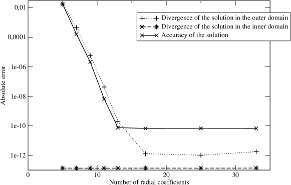
In Fig. 1, we observe as expected an exponential convergence of both the discrepancy between the theoretical and numerical solutions (maximum over all grid points and all components) as functions of the number of spectral coefficients used in the radial direction $N_{r}$, all other parameters being fixed. The same behavior has been observed when keeping $N_{r}$ fixed and varying $N_{\theta}$. Besides, we observe an exponential decay of the divergence of the solution in the second (or outer) domain, whereas the divergence of the solution in the first (central) domain remains constant to the radial precision. This is due to the matching across domains and imposition of boundary conditions, which can be seen as a modification of the solution of the system (37) by the addition of a linear combination of homogeneous solutions. These homogeneous solutions of the system (37) are, for each multipole $\ell$, $r^{\ell-1}$ and $1/r^{\ell+2}$. The latter being singular at $r=0$ is not relevant in the central domain. The $r^{\ell-1}$ function is a polynomial and is well represented in the first domain, whereas in the second domain, we also need to resolve $1/r^{\ell+2}$, which is poorly approximated for low values of $N_{r}$.

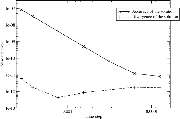
On the other hand, when varying the time-step $dt$, the difference between the numerical and exact solutions decreases as $\mathcal{O}(dt^{3})$ (see Fig. 2), as expected for a third-order scheme. Another feature verified in Fig. 2 is the fact that the divergence of the solution is (almost) independent of the time-step, being thus only a function of the spatial resolution. The best accuracy observed in Fig. 1 is limited by angular resolution and the fact that the divergence is computed using spherical components (Eq. 12), whereas the divergence-free constraint is imposed using pure spin components (Eq. 24). Therefore, the computation of derivatives in Eqs. (21) to obtain the spherical components introduces additional numerical noise, depending on the angular resolution.

5.3 Divergence-free and traceless tensor wave equation

Figure 3: Decay of the errors (difference with theoretical solution and divergence of the numerical solution) for the tensor wave equation, as a function of the number of radial Chebyshev coefficients $N_{r}$ used in each domain. Other settings are $R=6,dt=0.00032,N_{\theta}=17,N_{\varphi}=4$.

Similarly to Sec. 5.2, we consider here the numerical solution of the problem (39)-(41), with $\alpha_{0}^{ij}(r,\theta,\varphi)$ given in the Cartesian basis by (with $z=r\cos(\theta)$):

$$\alpha_{0}^{xx}=-\alpha_{0}^{yy}=\cos(z),$$ (100)

all the other components are zero. Thus the tensor $\alpha_{0}^{ij}$ is clearly symmetric, divergence-free and trace-free. With $\gamma_{0}^{ij}=0$ and appropriate boundary conditions, the solution of the problem (39)-(41) is (still in Cartesian components) simple to express:

$$h^{xx}(t,r,\theta,\varphi)=-h^{yy}(t,r,\theta,\varphi)=\cos(t)\cos(z),$$ (101)

all the other components being zero. The tensor wave equation is solved through the two scalar wave-like equations for the potentials $\mathcal{A}$ and $\tilde{\mathcal{B}}$ as explained in Sec. 3.4. From Eq. (101), we know the values of $\beta_{0}^{ij}(t,\theta,\varphi)$ appearing in Eq. (41) as Dirichlet boundary conditions and we can deduce its pure spin components $\left(\beta_{0}^{rr},\beta_{0}^{\eta},\beta_{0}^{\mu}\right)$. These are used to obtain Dirichlet boundary conditions for the evolution equations for $\mathcal{A}$ and $\tilde{\mathcal{B}}$, as described in Sec. 4.2 using Eqs. (89) and (96), respectively. Finally, the elliptic systems (80)-(84) are solved with the appropriate Dirichlet boundary conditions given by the spin components of $\beta_{0}^{ij}$, namely $\beta_{0}^{rr}$ and $\beta_{o}^{\mu}$.

Figure 4: Decay of the errors (difference with theoretical solution and divergence of the numerical solution) for the tensor wave equation, as a function of the time-step $dt$. Other settings are $R=6,N_{r}=17,N_{\theta}=17,N_{\varphi}=4$.

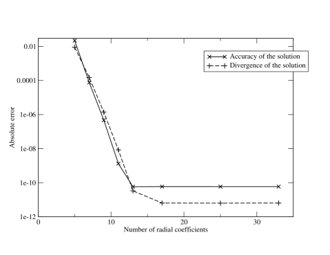
We have integrated the tensor wave equation following the same procedure as in Sec. 5.2. results are displayed in Figs. 3 and 4, where we observe as expected an exponential convergence of both the discrepancy between the theoretical and numerical solutions, and the divergence of the numerical, as functions of $N_{r}$. When varying the time-step $dt$, the difference between the numerical and exact solutions decreases as $\mathcal{O}(dt^{3})$, as expected. Here again, the divergence of the solution is (almost) independent of the time-step, being thus only a function of the spatial resolution, from the same reasons as in the vector case.

6 Concluding remarks

We have described a new numerical method for solving the wave equation of a rank-two symmetric tensor on a spherical grid, ensuring the divergence-free condition on this tensor. In order to describe this method, we have first addressed the vector case, for which we have reformulated the poloidal-toroidal decomposition in spherical components. This approach, which relies on a decomposition onto vector spherical harmonics was then generalized to the case of a symmetric tensor. Through numerical tests of the vector and tensor wave evolution in a sphere using spectral explicit time schemes, we have observed that this method was convergent and accurate. In particular, the level at which the divergence-free condition is violated is determined only by the spatial discretization and does not depend on the time-step, as expected. This method strongly relies on the decomposition onto spherical harmonic spectral bases, but is not bound to spectral methods for the representation of the radial coordinate.

The discussion in Sec. 4 gave us the compatibility conditions (86), (89) (96), which are necessary to obtain boundary conditions for the additional scalar field equations, representing the evolution of the divergence-free degrees of freedom of our objects ($A,\mathcal{A},\tilde{\mathcal{B}}$). The numerical tests performed in this study have dealt only with simple Dirichlet boundary conditions. However, it would be rather straightforward to generalize them to more complex boundary conditions, which are needed in realistic simulations of gravitational waves [18, 22, 23].

In this respect, an interesting issue would probably be the general well-posed nature of these boundary conditions with respect to our scheme, and how the modifications for these conditions with this method, sketched in Sec.4.1 and 4.2, would alter the physical behavior of the solution. One could for example think of a Robin-like boundary setting linked to an outer wave-absorbing condition (as in [22]), instead of the Dirichlet setting studied here; the fact that boundary conditions may be only partially verified could have an effect on how this required feature at the boundary would be described eventually in our scheme. The same type of questions arise in a more general case, where the source terms of the equations are non-vanishing: these sources would also require well-posedness conditions (i.e. a vanishing divergence for the wave equation). If this requirement is not satisfied (because of the iteration procedure or numerical errors), although the problem is then mathematically ill-posed, our scheme will still converge: it provides us with a solution of the wave equation with a source that is basically the divergence-free part of the original ill-posed source. The influence of this feature on the general stability and physical relevance of the procedure is an open issue.

Future studies include the simulations of perturbed black hole spacetimes, with the extraction of gravitational waves, and the solution of general-relativistic magneto-hydrodynamics in the case of a rotating neutron star.

References

- [1] M. Alcubierre, Introduction to numerical relativity, Oxford University Press, Oxford, 2008.
- [2] J. B. Boyd, Chebyshev and Fourier Spectral Methods, second ed., Dover, 2001.
- [3] S. Bonazzola, L. Villain, M. Bejger, Magnetohydrodynamics of rotating compact stars with spectral methods: description of the algorithm and tests , Class. Quantum Grav. 24 (2007) S221-S234.
- [4] S. Bonazzola, E. Gourgoulhon, P. Grandclément, J. Novak, Constrained scheme for the Einstein equations based on the Dirac gauge and spherical coordinates, Phys. Rev. D 70 (2004) 104007.
- [5] S. Bonazzola, J.-A. Marck, Three-dimensional gas dynamics in a sphere, J. Comput. Phys. 87 (1990) 201-230.
- [6] P. Boronski, L. S. Tuckerman, Poloidal-toroidal decomposition in a finite cylinder I: Influence matrices for the magnetohydrodynamic equation, J. Comput. Phys. 227 (2007) 1523-1543.
- [7] P. Boronski, L. S. Tuckerman, Poloidal-toroidal decomposition in a finite cylinder II: Discretization, regularization and validation, J. Comput. Phys. 227 (2007) 1544-1566.
- [8] T. de Donder, La gravifique Einsteinienne, Ann. Obs. R. Belg. (1921).
- [9] P. A. M. Dirac, Fixation of Coordinates in the Hamiltonian Theory of Gravitation, Phys. Rev. 114 (1959) 924-930.
- [10] E. Dormy, P. Cardin, D. Jault, MHD flow in a slightly differentially rotating spherical shell, with conducting inner core, in a dipolar magnetic field, Earth Plan. Sci. Lett. 160 (1998) 15-30.
- [11] M. Dudley, R. James,Time-dependent kinematic dynamos with stationary flows, Proc. Roy. Soc. London A 425 (1989) 407-429.
- [12] C. R. Evans, J. F. Hawley, Simulation of magnetohydrodynamic flows: a constrained transport method, Astrophys. J. 332 (1988) 659-677.
- [13] P. Grandclément, S. Bonazzola, E. Gourgoulhon, J.-A. Marck, A multidomain spectral method for scalar and vectorial Poisson equations with noncompact sources, J. Comput. Phys. 170 (2001) 231-260.
- [14] P. Grandclément, J. Novak, Spectral methods for numerical relativity, Living Rev. Relativity 12 (2009) 1 [Online article]: cited on 22 January 2009, http://www.livingreviews.org/lrr-2009-1.
- [15] E. Hairer, S. D. Norsett and G. Wanner, Ordinary Differential Equations I, Springer-Verlag 1987.
- [16] J. S. Hesthaven, S. Gottlieb, D. Gottlieb, Spectral Methods for Time-Dependent Problems, Cambridge University Press, Cambridge, 2007.
- [17] R. Hollerbach and G. Rüdiger, The influence of Hall drift in the magnetic fields of neutron stars, Mon. Not. Roy. Astron. Soc. 337 (2002) 216.
- [18] S. R. Lau, Rapid evaluation of radiation boundary kernels for time-domain wave propagation on blackholes: theory and numerical methods, J. Comput. Phys. 199 (2004), 376-422.
- [19] http://www.lorene.obspm.fr
- [20] F. Marqués, On boundary conditions for velocity potentials in confined flows: Application to Couette flow, Phys. Fluid A 2 (1990) 729-737.
- [21] J. Mathews, Gravitational multipole radiation, J. Soc. Ind. Appl. Math. 10 (1962) 768-780.
- [22] J. Novak, S. Bonazzola, Absorbing boundary conditions for simulation of gravitational waves with spectral methods in spherical coordinates, J. Comput. Phys. 197 (2004) 186-196.
- [23] O. Rinne, L. T. Buchman, M. A. Scheel, H. P. Pfeiffer, Implementation of higher-order absorbing boundary conditions for the Einstein equations, Class. Quantum Grav. 26 (2009) 075009.
- [24] K. S. Thorne, Multipole expansion of gravitational radiation, Rev. Mod. Phys. 52 (1980) 299-339.
- [25] G. Tóth, The constraint in shock-capturing magnethydrodynamics codes, J. Comput. Phys. 161 (2000) 605-652.
- [26] N. Vasset, J Novak, J. L. Jaramillo, Excised black hole spacetimes: quasi-local horizon formalism applied to the Kerr example, Phys. Rev. D 79 (2009) 124010.
- [27] F. J. Zerilli, Tensor harmonics in canonical form for gravitational radiation and other applications, J. Math. Phys. 11 (1970) 2203-2208.