Decay of the Greenland Ice Sheet due to surface-meltwater-induced acceleration
of basal sliding

Abstract

Simulations of the Greenland Ice Sheet are carried out with a high-resolution version of the ice-sheet model SICOPOLIS for several global-warming scenarios for the period 1990–2350. In particular, the impact of surface-meltwater-induced acceleration of basal sliding on the stability of the ice sheet is investigated. A parameterization for the acceleration effect is developed for which modelled and measured mass losses of the ice sheet in the early 21st century agree well. The main findings of the simulations are: (i) the ice sheet is generally very susceptible to global warming on time-scales of centuries, (ii) surface-meltwater-induced acceleration of basal sliding leads to a pronounced speed-up of ice streams and outlet glaciers, and (iii) this ice-dynamical effect accelerates the decay of the Greenland Ice Sheet as a whole significantly, but not catastrophically, in the 21st century and beyond.

1 Introduction

In Chapter 10 (“Global Climate Projections”) of the Fourth Assessment Report (AR4) of the United Nations Intergovernmental Panel on Climate Change (IPCC), an increase of the mean global sea level by 18–59 cm for the 21st century (more precisely: 2090–2099 relative to 1980–1999) is projected for the six SRES marker scenarios B1, B2, A1B, A1T, A2 and A1FI (Meehl et al. 2007). The main causes for this sea level rise are thermal expansion of sea water and melting of glaciers and small ice caps, and to a lesser extent changes of the surface mass balance of the Greenland and Antarctic Ice Sheets. However, recent observations suggest that ice flow dynamics could lead to additional sea level rise, and this problem is explicitly stated in the AR4:

“Dynamical processes related to ice flow not included in current models but suggested by recent observations could increase the vulnerability of the ice sheets to warming, increasing future sea level rise. Understanding of these processes is limited and there is no consensus on their magnitude.” (IPCC 2007).

These conjectured dynamical processes are (i) basal sliding accelerated by surface meltwater, (ii) reduced buttressing due to the loss of ice shelves, and (iii) penetration of ocean water under the ice. The first process is more relevant for the Greenland Ice Sheet (the focus of this study), whereas the latter two may affect the stability of the West Antarctic Ice Sheet. On the observational side, recent results from satellite gravity measurements for the period 2002-2005 indicate surprisingly large mass losses of $239\pm{}23\;\mathrm{km^{3}\,a^{-1}}$ ($0.66\pm{}0.06\;\mathrm{mm\;a^{-1}}$ sea level equivalent) for the Greenland Ice Sheet (Chen et al. 2006). Furthermore, major outlet glaciers (Jacobshavn ice stream, Kangerdlugssuaq and Helheim glaciers) have sped up drastically since the 1990’s (Rignot and Kanagaratnam 2006).

2 Ice-sheet model SICOPOLIS

For this study, we use the ice-sheet model SICOPOLIS (“SImulation COde for POLythermal Ice Sheets”), which simulates the large-scale dynamics and thermodynamics (ice extent, thickness, velocity, temperature, water content and age) of ice sheets three-dimensionally and as a function of time (Greve 1997; http://sicopolis.greveweb.net/). It is based on the shallow-ice approximation (e.g. Hutter 1983) and the rheology of an incompressible, heat-conducting power-law fluid [Glen’s flow law, see Paterson (1994)]. External forcing is specified by (i) the mean annual air temperature at the ice surface, (ii) the surface mass balance (precipitation minus runoff), (iii) the sea level surrounding the ice sheet and (iv) the geothermal heat flux prescribed at the bottom of a lithospheric thermal boundary layer of 5 km thickness. For all simulations of this study, the horizontal resolution is 10 km, the vertical resolution is 81 grid points for the cold-ice column, 11 grid points for the basal layer of temperate ice (if existing) and 11 grid points for the lithosphere layer, the time-step is 0.25 a, and the geothermal heat-flux distribution and model parameters are those used by Greve (2005).

3 WRE1000 scenario

Future global warming shall be prescribed exemplarily by the WRE1000 scenario, which assumes stabilisation of the atmospheric CO₂ concentration at 1000 ppm (Cubasch et al. 2001). The corresponding temperature change from 1990 (the “present”) until 2350 is shown in Fig. 1 (along with similar scenarios with lower stabilisation concentrations).

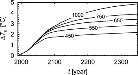
Figure 1: Global mean temperature change $\Delta{}T_{\mathrm{g}}$ for the scenarios WRE450, WRE550, WRE650, WRE750 and WRE1000 (stabilisation scenarios for atmospheric CO₂), by Cubasch et al. (2001). In this study, only the WRE1000 scenario will be considered.

In order to obtain temperature and precipitation forcings for the Greenland Ice Sheet, the argumentation by Greve (2004) is followed. The surface temperatures shown in Fig. 1 are amplified by a factor 2 and imposed as uniform increases over the ice sheet, and the precipitations are assumed to increase by $5\%$ per degree of ice-sheet-surface-temperature change. Surface melting is parameterized by the degree-day method in the version by Greve (2005). This approach is a critical simplification, and it should rather be replaced by an energy-balance model for more accurate results. However, since the objective of this study is to assess the impact of ice-dynamical processes on the decay of the Greenland Ice Sheet rather than making precise predictions of the decay itself, the use of the degree-day method is a reasonable compromise.

4 Basal sliding

Basal sliding is described by a Weertman-type sliding law in the form of Greve and Otsu (2007), based on Greve et al. (1998) and modified to allow for sub-melt sliding (Hindmarsh and Le Meur 2001),

$$v_{\mathrm{b}}=-C_{\mathrm{b}}\,\mathrm{e}^{T^{\prime}_{\mathrm{b}}/\gamma_{\mathrm{sms}}}\times\frac{\tau_{\mathrm{b}}^{3}}{P_{\mathrm{b}}^{2}}\,,$$ (1)

where $v_{\mathrm{b}}$ is the basal-sliding velocity, $C_{\mathrm{b}}$ the sliding coefficient, $\tau_{\mathrm{b}}$ the basal shear traction in the bed plane, $\rho$ the ice density, $g$ the gravity acceleration, $H$ the ice thickness and $P_{\mathrm{b}}{=}\rho{}gH$ the overburden pressure. The term $e^{T^{\prime}_{\mathrm{b}}/\gamma_{\mathrm{sms}}}$ represents the exponentially diminishing sub-melt sliding, where $T^{\prime}_{\mathrm{b}}$ is the temperature relative to pressure melting (in ${}^{\circ}\mathrm{C}$) and $\gamma_{\mathrm{sms}}{=}1^{\circ}\mathrm{C}$ the sub-melt-sliding coefficient.

Acceleration of basal sliding by surface meltwater is parameterized by an extension of the approach by Greve and Otsu (2007). The sliding coefficient is expressed as

$$C_{\mathrm{b}}=C_{\mathrm{b}}^{0}\,\left(1+\frac{\gamma}{H^{r}}M^{s}\right)\,,$$ (2)

where $C_{\mathrm{b}}^{0}=11.2\,\mathrm{m\,a^{-1}\,Pa^{-1}}$, $M$ is the surface melt rate (runoff), $\gamma$ is the surface meltwater coefficient, and $r$ and $s$ are adjustable exponents. The idea behind this parameterization is to relate the sliding speed-up to the local surface melt rate, and account for the less efficient percolation of meltwater to the base in regions where the ice is thick by the dependency on the inverse ice thickness.

The parameterization employed by Greve and Otsu (2007) corresponds to $(r,s)=(0,1)$. For this case, the authors show in their Appendix A that data reported by Zwally et al. (2002) from the Swiss Camp in central west Greenland give rise to the estimate $\gamma=0.1\;\mathrm{a\;m^{-1}}$. We will also consider the cases $(r,s)=(0,2)$ and $(1,1)$, for which the same arguments lead to estimates of $\gamma=0.05\;\mathrm{a^{2}\;m^{-2}}$ and $100\;\mathrm{a}$, respectively.

5 Simulations

5.1 Set-up

Five simulations with different settings for the acceleration of basal sliding by surface meltwater will be discussed in order to investigate to what extent this process can increase the vulnerability of the Greenland Ice Sheet to future warming. In run #1, acceleration of basal sliding by surface meltwater is not considered ($\gamma=0$). Runs #2-4 have been conducted with $(r,s)=(0,1)$, $(0,2)$ and $(1,1)$, respectively, and values of $\gamma$ chosen according to the estimates given at the end of Sect. 4 (designated in Table 1 as “100%”). Run #5 corresponds to the most extreme scenario considered by Greve and Otsu (2007), with the settings $(r,s)=(0,1)$ and $\gamma=5\;\mathrm{a\;m^{-1}}$ (50 times the above estimate, therefore designated in Table 1 as “5000%”). All simulations start with the present-day ice sheet as initial condition, and the model time is from 1990 until 2350.

Run	$\gamma$	$(r,s)$	$\dot{V}_{\mathrm{2002-2005}}$	$\Delta{}V_{\mathrm{2100}}$	$\Delta{}V_{\mathrm{2200}}$	$\Delta{}V_{\mathrm{2300}}$
			$[\mathrm{km^{3}\,a^{-1}}]$	$[\mathrm{m\;SLE}]$	$[\mathrm{m\;SLE}]$	$[\mathrm{m\;SLE}]$
#1	$\,0$	—	$\;\;37.7$	$0.12$	$0.55$	$1.21$
#2	$100\%$	$(0,1)$	$111.6$	$0.14$	$0.60$	$1.31$
#3	$100\%$	$(0,2)$	$172.0$	$0.17$	$0.68$	$1.48$
#4	$100\%$	$(1,1)$	$248.9$	$0.18$	$0.67$	$1.42$
#5	$5000\%\;\;$	$(0,1)$	$1627.8\;\,$	$0.58$	$1.51$	$2.71$

Table 1: Set-up and results of runs #1-5. For the meaning of the basal-sliding parameters $\gamma$, $r$, $s$ see Eq. (2) and the accompanying text. $\dot{V}_{\mathrm{2002-2005}}$ denotes the average loss of ice volume between 2002 and 2005, whereas $\Delta{}V_{\mathrm{2100}}$, $\Delta{}V_{\mathrm{2200}}$ and $\Delta{}V_{\mathrm{2300}}$ are the losses of ice volume by 2100, 2200 and 2300, respectively, compared to 1990. The latter are expressed in meters of sea-level equivalent.

5.2 Results

An overview of the main results is given in Table 1. The average loss of ice volume between 2002 and 2005 can be compared with the measured value by Chen et al. (2006) of $239\pm{}23\;\mathrm{km^{3}\,a^{-1}}$ (see introduction), thus providing an observational constraint for the simulations. Evidently, the ice-volume loss is far too small for run #1 (no acceleration of basal sliding by surface meltwater), and it is too small by about a factor 2 for run #2 [$(r,s)=(0,1)$]. By contrast, the agreement is quite good for run #3 [$(r,s)=(0,2)$] and very good for run #4 [$(r,s)=(1,1)$]. On the other hand, the extreme case of run #5 [$(r,s)=(0,1)$, very large $\gamma$] produces more than 6 times more ice-volume loss than observed. Therefore, runs  #3 and 4 seem to be most realistic.

From a theoretical point of view, the set-up of run #4 is preferable to that of run #3, because it is clear that the percolation of surface meltwater to the base will be the less efficient the thicker the ice is. This is accounted for in run #4, for which the acceleration of basal sliding decreases with increasing ice thickness ($r=1$), whereas this is not the case in run #3 ($r=0$). Consequently, run #4 shall be considered as the “best” simulation.

Comparison of the results of run #4 and run #1 (no acceleration of basal sliding by surface meltwater) shows that the contribution to sea-level rise by 2100 is $\sim{}50\%$ larger for run #4 (0.18 vs. 0.12 m). The impact of the acceleration effect on ice flow becomes evident by inspection of Fig. 2 which shows the simulated surface velocities in 2100 for the two runs. Therefore, the acceleration of basal sliding by surface meltwater, which is most likely the major ice-dynamical process relevant for the Greenland Ice Sheet in the context of global warming, has a significant, but not catastrophic effect on the decay of the ice sheet in the 21st century.

The absolute difference between the two runs becomes larger in the more distant future; however, the relative difference becomes smaller: by 2200 the contribution to sea-level rise is 0.12 m ($\sim{}22\%$) larger for run #4, and by 2300 it is 0.21 m ($\sim{}17\%$) larger. Figure 3 shows the simulated surface topographies in 2350 (at the end of the simulations). It is nicely illustrated that for both runs  #1 and #4 the ice sheet shows a strong response on the imposed warming scenario and retreats all around the margin (most pronounced in the south-west), while the surface-meltwater-induced acceleration of basal sliding accounted for in run  #4 speeds up the decay.

Two additional simulations with larger exponents, namely $(r,s)=(1,2)$ and $(2,1)$, and values of $\gamma$ chosen in analogy to the “100%” runs #2-4, have also been conducted. For these cases, maximum surface velocities of more than $100\;\mathrm{km\,a^{-1}}$ occur close to the ice margin, which is unrealistic. Apparently, the speed-up effect is too pronounced for these settings, and so they have been discarded.

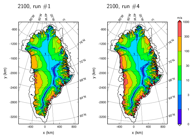
Figure 2: Simulated surface velocity of the Greenland Ice Sheet. Left: Run #1 (no acceleration of basal sliding by surface meltwater), year 2100. Right: Run #4 (“best” simulation, including acceleration of basal sliding by surface meltwater), year 2100. Both simulations reproduce the organization of the drainage pattern into ice streams and outlet glaciers, despite the use of the shallow-ice approximation and the large-scale (10 km) resolution. The dynamic acceleration effect in run #4 is clearly visible all around the ice margin and leads to faster decay.

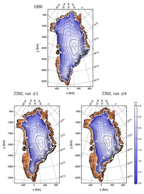
Figure 3: Simulated surface topography of the Greenland Ice Sheet. Top: Initial condition for the year 1990. Bottom left: Run #1 (no acceleration of basal sliding by surface meltwater), year 2350. Bottom right: Run #4 (“best” simulation, including acceleration of basal sliding by surface meltwater), year 2350. The difference between 1990 and 2350 amounts to $1.59\;\mathrm{m\;SLE}$ for run #1 and to $1.84\;\mathrm{m\;SLE}$ for run #4.

6 Conclusion

The simulations discussed in this study suggest that ice-dynamical processes can speed up the decay of the Greenland Ice Sheet significantly in the 21st century and beyond. However, a catastrophically accelerated decay can only be obtained with unrealistic parameter settings and thus seems to be unlikely.

References

- Chen et al. (2006) Chen, J. L., C. R. Wilson and B. D. Tapley. 2006. Satellite gravity measurements confirm accelerated melting of Greenland ice sheet. Science, 313 (5795), 1958–1960. doi:10.1126/science.1129007.
- Cubasch and 8 others (2001) Cubasch, U. and 8 others. 2001. Projections of future climate change. In: J. T. Houghton and 7 others (Eds.), Climate Change 2001: The Scientific Basis. Contribution of Working Group I to the Third Assessment Report of the Intergovernmental Panel on Climate Change, pp. 525–582. Cambridge University Press, Cambridge, UK and New York, NY, USA.
- Greve (1997) Greve, R. 1997. Application of a polythermal three-dimensional ice sheet model to the Greenland ice sheet: Response to steady-state and transient climate scenarios. J. Climate, 10 (5), 901–918.
- Greve (2004) Greve, R. 2004. Evolution and dynamics of the Greenland ice sheet over past glacial-interglacial cycles and in future climate-warming scenarios. In: Proceedings of the 5th International Workshop on Global Change: Connection to the Arctic (GCCA5), pp. 42–45. University of Tsukuba, Japan. URL http://hdl.handle.net/2115/30204.
- Greve (2005) Greve, R. 2005. Relation of measured basal temperatures and the spatial distribution of the geothermal heat flux for the Greenland ice sheet. Ann. Glaciol., 42, 424–432.
- Greve and Otsu (2007) Greve, R. and S. Otsu. 2007. The effect of the north-east ice stream on the Greenland ice sheet in changing climates. The Cryosphere Discuss., 1 (1), 41–76. URL http://www.the-cryosphere-discuss.net/1/41/2007/.
- Greve et al. (1998) Greve, R., M. Weis and K. Hutter. 1998. Palaeoclimatic evolution and present conditions of the Greenland ice sheet in the vicinity of Summit: An approach by large-scale modelling. Paleoclimates, 2 (2-3), 133–161.
- Hindmarsh and Le Meur (2001) Hindmarsh, R. C. A. and E. Le Meur. 2001. Dynamical processes involved in the retreat of marine ice sheets. J. Glaciol., 47 (157), 271–282.
- Hutter (1983) Hutter, K. 1983. Theoretical Glaciology; Material Science of Ice and the Mechanics of Glaciers and Ice Sheets. D. Reidel Publishing Company, Dordrecht, The Netherlands.
- IPCC (2007) IPCC. 2007. Summary for policymakers. In: S. Solomon and 7 others (Eds.), Climate Change 2007: The Physical Science Basis. Contribution of Working Group I to the Fourth Assessment Report of the Intergovernmental Panel on Climate Change, pp. 1–18. Cambridge University Press, Cambridge, UK and New York, NY, USA.
- Meehl and 13 others (2007) Meehl, G. A. and 13 others. 2007. Global climate projections. In: S. Solomon and 7 others (Eds.), Climate Change 2007: The Physical Science Basis. Contribution of Working Group I to the Fourth Assessment Report of the Intergovernmental Panel on Climate Change, pp. 747–845. Cambridge University Press, Cambridge, UK and New York, NY, USA.
- Paterson (1994) Paterson, W. S. B. 1994. The Physics of Glaciers. Pergamon Press, Oxford, UK etc., 3rd ed.
- Rignot and Kanagaratnam (2006) Rignot, E. and P. Kanagaratnam. 2006. Changes in the velocity structure of the Greenland ice sheet. Science, 311 (5763), 986–990. doi:10.1126/science.1121381.
- Zwally et al. (2002) Zwally, H. J., W. Abdalati, T. Herring, K. Larson, J. Saba and K. Steffen. 2002. Surface melt-induced acceleration of Greenland ice-sheet flow. Science, 297 (5579), 218–222. doi:10.1126/science.1072708.