Heterogeneous viral environment
in a HIV spatial model

Abstract.

We consider the basic model of virus dynamics in the modeling of Human Immunodeficiency Virus (HIV), in a $2D$ heterogenous environment. It consists of two ODEs for the non-infected and infected $CD_{4}^{+}$ $T$-lymphocytes, $T$ and $I$, and a parabolic PDE for the virus $V$. We define a new parameter $\lambda_{0}$ as an eigenvalue of some Sturm-Liouville problem, which takes the heterogenous reproductive ratio into account. For $\lambda_{0}<0$ the trivial non-infected solution is the only equilibrium. When $\lambda_{0}>0$, the former becomes unstable whereas there is only one positive infected equilibrium. Considering the model as a dynamical system, we prove the existence of a universal attractor. Finally, in the case of an alternating structure of viral sources, we define a homogenized limiting environment. The latter justifies the classical approach via ODE systems.

Claude-Michel Brauner

Institut de Mathématiques de Bordeaux

Université de Bordeaux, 33405 Talence cedex (France)

Danaelle Jolly

Institut de Mathématiques de Bordeaux

Université de Bordeaux, 33405 Talence cedex (France)

Luca Lorenzi

Dipartimento di Matematica

Università di Parma, Viale G.P. Usberti 53/A, 43100 Parma (Italy)

Rodolphe Thiebaut

(M.D.) Equipe Biostatistique de l’U897 INSERM ISPED

Université de Bordeaux, 33076 Bordeaux cedex (France)

1. Introduction

The acute infection by the Human Immunodeficiency Virus (in short HIV) is characterized by a huge depletion of the $CD_{4}^{+}~{}T$-lymphocytes ($CD_{4}$) and a peak of the virus load [7]. After few weeks, these two components reach a steady state which characterizes the asymptomatic phase of the infection. Before the availability of highly active antiretroviral therapy, this later phase lasted after $10$ years in median with an accelerated decrease of $CD_{4}$ and an increase of virus load. A substantial number of nonlinear ODE systems have been suggested by Perelson et al. (see [21, 22]) to model the complex dynamics of HIV-host interaction. For instance, such models have been used to estimate the infected cell half-life and the viral clearance during antiretroviral therapy [11, 20, 29], or to understand the dynamics during acute infection [23].

The common basic model of viral dynamics [2] includes three variables: $T$, the non-infected $CD_{4}$, $I$, the infected $CD_{4}$, and $V$, the free virus:

$$T_{t}=\alpha-\gamma VT-\mu_{T}T,$$ (1.1a)

$$I_{t}=\gamma VT-\mu_{I}I,$$ (1.1b)

$$V_{t}=N\mu_{I}I-\mu_{V}V.$$ (1.1c)

This model, describing the interaction between the replicating virus of HIV and host cells, is based on some simple hypotheses. Non-infected target cells are produced by the thymus at a constant rate $\alpha$ and die at a rate $\mu_{T}$. By contact with the free virus particles (virions) they become infected at a rate proportional to their abundance, $\gamma VT$ (see Fig. 1). These infected cells die at a rate $\mu_{I}$ and produce free viruses during their life-time at a rate $N$. Free particles are removed at a rate called the clearance $\mu_{V}$. All these parameters are generally positive constants. This simple model study has led to interesting results (see [18, 28]) and suggested a treatment strategy (see [2]).

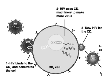
Figure 1. The HIV life cycle

It is easily seen that the system has two equilibria:

1. the non-infected steady state

   $$T_{u}=\frac{\alpha}{\mu_{T}},\quad I_{u}=0,\quad V_{u}=0,$$

   which corresponds to a non-negative equilibrium in case of no infection;

2. the infected steady state

   $$T_{i}=\frac{\mu_{V}}{\gamma N},\quad I_{i}=\frac{\alpha\gamma N-\mu_{T}\mu_{V}}{\gamma N},\quad V_{i}=\frac{\alpha\gamma N-\mu_{T}\mu_{V}}{\gamma\mu_{V}},$$ (1.2)

   also called seropositivity steady state, corresponding to a positive equilibrium in case of infection.

Some authors (see e.g., [2, 18]) have considered the basic reproductive ratio $R_{0}$:

$$R_{0}=\frac{\gamma\alpha N}{\mu_{T}\mu_{V}},$$ (1.3)

a dimensionless parameter defined by epidemiologists as the average number of infected cells that derive from any one infected cell in the beginning of the infection [18, p. 16]. Stability properties of the two steady states are usually studied around this quantity: if $R_{0}<1$ the non-infected steady state is stable, if $R_{0}>1$ the infected steady state has a biological meaning and it is stable, while at $R_{0}=1$ both steady states coincide. So, $R_{0}=1$ is a bifurcation point (see Fig. 2).

Figure 2. Typical bifurcation diagram, with $R_{0}$ varying between $0$ and $3$, as a function of $\alpha$. The solid line represents the stable branch of $V$, the dashed line the unstable one. The other parameters have the values: $\gamma=0.001,~{}N=1000,~{}\mu_{T}=0.1,~{}\mu_{I}=0.5,~{}\mu_{V}=10$.

Figure 3. Profiles of virus (left) and target cells (right) in the case of infection. Here $R_{0}=1.5$ and the other parameters have the same values as in Fig. 2.

Further models have been used involving other populations present in the immune system (see [17, 18, 4]). However, these models assume that the populations $T,~{}I,~{}V$ are homogeneous over the space for all time, which is a common, but not a very realistic, assumption. Actually, the interaction between the virus and the immune system (either as a target with $CD_{4}$ or as an agent for controlling infection) is localized according to the type of tissues [3] and also in a given tissue (e.g. lymph nodes). To examine the effects of both diffusion and spatial heterogeneity, Funk et al. [8] introduced a discrete model based on (1.1a)-(1.1c). These authors adopted a two-dimensional square grid with $21\times 21$ sites and assumed that the virus can move to the eight nearest neighboring sites. They pointed out that the presence of a spatial structure enhances population stability with respect to non-spatial models. However, our analysis does not confirm this observation (see Section 4 below).

Recently, Wang et al. [26] generalized Funk et al.’s model. They assumed that the hepatocytes can not move under normal conditions and neglected their mobility, while viruses can move freely and their motion follows a Fickian diffusion. They proposed the following system of two ODEs coupled with a parabolic PDE for the virus:

$$T_{t}=\alpha-\gamma VT-\mu_{T}T,$$ (1.4a)

$$I_{t}=\gamma VT-\mu_{I}I,$$ (1.4b)

$$V_{t}=N\mu_{I}I-\mu_{V}V+d_{V}\Delta V,$$ (1.4c)

where $d_{V}$ is the diffusion coefficient. They assumed that the domain is the whole real line and proved the existence of traveling waves. Wang et al. [27] introduced a delay to take into account the time between infection of a target cell and the emission of viral particles [6]. They considered (1.4a)-(1.4c) in a one-dimensional interval with Neumann boundary conditions.

In the spirit of the above works, we intend to study System (1.4a)-(1.4c) in a two-dimensional spatial domain $(0,\ell)\times(0,\ell)$ with periodic boundary conditions. There are two main situations:

1. the environment is homogeneous and, hence, all the parameters in (1.4a)-(1.4c) are constant. Therefore, the system with diffusion has the same equilibria as System (1.1a)-(1.1c);

2. the environment is heterogeneous, therefore certain parameters become positive functions of the space variable. Then, the virus is spatially structured.

For simplicity, we assume throughout the paper that only the rate $\alpha$ varies while the other parameters are fixed positive constants. In fact, it is biologically plausible to assume that the arrival of new $CD_{4}$ may vary according to local areas. More precisely, $\alpha$ is piecewise continuous and periodic in each variable with period $\ell$. Then it is convenient to define the heterogeneous reproductive ratio:

$$R_{0}(x)=\frac{\gamma N\alpha(x)}{\mu_{T}\mu_{V}},\qquad\;\,x\in(0,\ell)\times(0,\ell).$$ (1.5)

The sites where $R_{0}(x)<1$ are called sinks while the sites where $R_{0}(x)>1$ are called sources [8].

The paper is organized as follows. In Section 2 we are interested in the stationary problem associated with (1.4a)-(1.4c) and its non-negative equilibria. The virus equilibrium verifies the elliptic semilinear equation

$$d_{V}\Delta V-\mu_{V}V=-\mu_{T}\mu_{V}R_{0}(x)\frac{V}{\gamma V+\mu_{T}},$$ (1.6)

with periodic boundary conditions. A first issue is to define a parameter which will play the role of the bifurcation parameter $R_{0}$ in the case the latter is constant. A candidate for this role is the largest eigenvalue $\lambda_{0}$ of the operator:

$$d_{V}\Delta+\mu_{V}(R_{0}-1)Id,$$ (1.7)

which is the linearization around $V\equiv 0$ of (1.6). For the reader’s convenience, we recall some basic facts about two-dimensional Sturm-Liouville eigenvalue problems with periodic boundary conditions such as (1.7) and give some proofs in Appendix A.

It is clear that, whenever $R_{0}$ is a constant, $\lambda_{0}=\mu_{V}(R_{0}-1)$. Therefore, we distinguish two cases, depending upon the sign of $\lambda_{0}$:

1. $\lambda_{0}\leq 0$: the trivial non-infected solution $V_{u}\equiv 0$ is the only solution of (1.6);

2. $\lambda_{0}>0$: (1.6) has exactly two non-negative solutions, namely the trivial non-infected solution $V_{u}\equiv 0$ and the positive infected solution $V_{i}$.

Section 3 is devoted to the study of the evolution problem (1.4a)-(1.4c). In the case $\lambda_{0}<0$, we prove that the trivial non-infected solution $(T_{i},I_{i},V_{i})$ is asymptotically stable. Then, we turn our attention to the biologically relevant case $\lambda_{0}>0$. First, we prove the non-infected solution becomes unstable. Second, we consider (1.4a)-(1.4c) as a dynamical system and prove the existence of an universal (or maximal) attractor. Since the system is only partly dissipative, we use a result of Marion [16]. The following Section 4 is devoted to some special cases where the positive infected solution $V_{i}$ is stable. Particular attention is paid to the case when $R_{0}$ is a constant: in this case discrete Fourier transform can be applied.

We point out that our proof can be extended to further models in HIV literature. It is not difficult to take a logistic term into account in the $T$ equation [22], although the steady equation (1.6) will be more involved. Adding such a term, Hopf bifurcations have been observed numerically in ODE systems (see [20]). Therefore, proving the stability of the infected solution may be, in general, challenging.

In the last section (Section 5), we consider the case when a heterogeneous environment is formed of sinks and sources alternating very rapidly, with a heterogeneous reproductive ratio $R_{0}(\frac{x}{\varepsilon})$. We determine the homogenized limiting medium as $\varepsilon\to 0$. It is fully characterized by a constant reproductive ratio, the mean value of $R_{0}$. Therefore, the classical approach of HIV dynamics via ODEs in a homogenous environment can be a posteriori justified in this respect.

Notation

Throughout this paper, for any $\ell>0$, we denote by $L^{2}$ the usual space of functions $f:(0,\ell)^{2}\to\mathbb{R}$ such that $f^{2}$ is integrable. The square $(0,\ell)^{2}$ will be simply denoted by $\Omega_{\ell}$. By $H^{k}$ we denote the Sobolev space of order $k$, i.e., the subset of $L^{2}$ of all the functions whose distributional derivatives up to $k$-th order are in $L^{2}$. Both $L^{2}$ and $H^{2}$ are endowed with their Euclidean norm. Finally, by $H^{k}_{\sharp}$ we denote the closure in $H^{k}$ of the space $C^{m}_{\sharp}$ of all $m$-th continuously differentiable functions $f:{\mathbb{R}}^{2}\to{\mathbb{R}}$ which are periodic with period $\ell$ in each variable. The space $H^{k}_{\sharp}$ is endowed with the norm of $H^{k}$. Finally, we denote by $Id$ the identity operator.

2. A semilinear equation for the virus steady states: existence and uniqueness of the equilibria

We start from the system for the virus dynamics:

$$T_{t}=\alpha-\gamma VT-\mu_{T}T,$$ (2.1a)

$$I_{t}=\gamma VT-\mu_{I}I,$$ (2.1b)

$$V_{t}=N\mu_{I}I-\mu_{V}V+d_{V}\Delta V,$$ (2.1c)

set in $\Omega_{\ell}$. Periodic boundary conditions for $T,I$ and $V$ are prescribed.

We are interested in the existence of steady state solutions to the equations (2.1a)-(2.1c) which belong to the space $L^{2}\times L^{2}\times H^{2}_{\sharp}$. Clearly, any steady state solution to Problem (2.1a)-(2.1c) is a solution to the following stationary system:

$$\alpha-\gamma VT-\mu_{T}T=0,$$ (2.2a)

$$\gamma VT-\mu_{I}I=0,$$ (2.2b)

$$N\mu_{I}I-\mu_{V}V+d_{V}\Delta V=0.$$ (2.2c)

From a biological point of view, only non-negative solutions to (2.2a)-(2.2c) have a meaning. Hence, we limit ourselves to proving the existence of this kind of steady state solutions.

System (2.2a)-(2.2c) can be reduced to a single scalar equation for the unknown $V$. Actually, it is not difficult to infer from (2.2a), (2.2b) that

$$T=\frac{\alpha}{\gamma V+\mu_{T}},\quad I=\frac{\gamma\alpha V}{\mu_{I}(\gamma V+\mu_{T})}.$$

Hence, the function $V$ turns out to solve the equation

$$d_{V}\Delta V-\mu_{V}V=-\frac{\gamma\alpha NV}{\gamma V+\mu_{T}}=-\mu_{T}\mu_{V}R_{0}\frac{V}{\gamma V+\mu_{T}},$$ (2.3)

associated with periodic boundary conditions.

2.1. Existence and uniqueness of non-negative equilibria

In this subsection we will provide a thorough study of the equation (2.3). As it has been already stressed, we are interested in non-negative solutions only.

Clearly, equation (2.3) always admits the trivial non-infected solution $V\equiv 0$ and, hence, Problem (2.1a)-(2.1c) admits

$$T_{u}(x)=\frac{\alpha(x)}{\mu_{T}},\qquad I_{u}(x)=0,\qquad V_{u}(x)=0,\qquad\;\,x\in\Omega_{\ell},$$ (2.4)

as a (trivial) steady state solution. We will call the triplet $(T_{u},I_{u},V_{u})$ the non-infected solution.

We are interested in studying the uniqueness of the non-infected solution in the class of all the non-negative steady state solutions to Problem (2.1a)-(2.1c). Of course, in the case when uniqueness does not hold (a situation which can actually occur, look for instance at the case when $R_{0}>1$ and $\alpha$ is constant, discussed in the introduction) we want to characterize all biological relevant steady state solutions to Problem (2.1a)-(2.1c).

For this purpose, we need to recall the following results about Sturm-Liouville eigenvalue problems in dimension two with periodic boundary conditions.

Theorem 2.1.

Let $d$ and $\mu$ be, respectively, a positive constant and a bounded measurable function. Further, let ${\mathscr{A}}:H^{2}_{\sharp}\to L^{2}$ be the operator defined by ${\mathscr{A}}u=d\Delta u-\mu u$ for any $u\in H^{2}_{\sharp}$. Then, the spectrum of ${\mathscr{A}}$ consists of eigenvalues only. Moreover, its maximum eigenvalue $\lambda_{\max}$ is given by the following formula:

$$\lambda_{\max}=-\inf_{\psi\in H^{1}_{\sharp},\psi\not\equiv 0}\left\{\frac{d\int_{\Omega_{\ell}}|\nabla\psi|^{2}dx+\int_{\Omega_{\ell}}\mu\psi^{2}dx}{\int_{\Omega_{\ell}}\psi^{2}dx}\right\}.$$ (2.5)

Finally, the eigenspace corresponding to the eigenvalue $\lambda_{\max}$ is one dimensional and contains functions which do not change sign in $\overline{\Omega_{\ell}}$.

This is a rather classical result. Nevertheless, for the reader’s convenience, we give a proof in Appendix A.

In view of Theorem 2.1, we can define the constant $\lambda_{0}$ to be the maximum eigenvalue of the operator $\varphi\mapsto d_{V}\Delta\varphi+\mu_{V}(R_{0}-1)\varphi$, which is the linearization around $V\equiv 0$ of operator $V\mapsto d_{V}\Delta V-\mu_{V}V+\mu_{T}\mu_{V}R_{0}\frac{V}{\gamma V+\mu_{T}}$. According to (2.5),

$$-\lambda_{0}=\inf_{\psi\in H^{1}_{\sharp},\psi\not\equiv 0}\left\{\frac{d_{V}\int_{\Omega_{\ell}}(\psi_{x})^{2}dx+\mu_{V}\int_{\Omega_{\ell}}(1-R_{0})\psi^{2}dx}{\int_{\Omega_{\ell}}\psi^{2}dx}\right\}.$$ (2.6)

As we are going to show, the uniqueness of the non-infected steady state solution is related to the value of $\lambda_{0}$.

Lemma 2.2.

If $\lambda_{0}\leq 0$, then the non-infected solution $(T_{u},I_{u},V_{u})$ $($see (2.4)$)$ is the only non-negative solution of (2.1a)-(2.1c).

Proof.

We argue by contradiction. Let us suppose that Problem (2.2a)-(2.2c) admits another solution $(T^{*},I^{*},V^{*})$ different from $(T_{u},I_{u},V_{u})$. Then, the function $V^{*}\in H^{2}_{\sharp}$ does not identically vanish in $\Omega_{\ell}$ and it solves the equation (2.3). Multiplying both the sides of this equation by $V^{*}$ and integrating by parts in $\Omega_{\ell}$, we get:

$$d_{V}\int_{\Omega_{\ell}}|\nabla V^{*}|^{2}dx+\mu_{V}\int_{\Omega_{\ell}}\left(1-\frac{\mu_{T}R_{0}}{\gamma V^{*}+\mu_{T}}\right)(V^{*})^{2}dx=0,$$

or, equivalently,

$$d_{V}\int_{\Omega_{\ell}} |\nabla V^{*}|^{2}dx+\mu_{V}\int_{\Omega_{\ell}}\left(1-R_{0}\right)(V^{*})^{2}dx$$

$$+\mu_{V}\int_{\Omega_{\ell}}R_{0}\left(1-\frac{\mu_{T}}{\gamma V^{*}+\mu_{T}}\right)(V^{*})^{2}dx=0.$$

Since $V^{*}$ does not identically vanish in $\Omega_{\ell}$, the last integral term is positive, implying that

$$d_{V}\int_{\Omega_{\ell}}|\nabla V^{*}|^{2}dx+\mu_{V}\int_{\Omega_{\ell}}\left(1-R_{0}\right)(V^{*})^{2}dx<0.$$

Hence, the infimum in (2.5) is negative which contradicts our assumption $-\lambda_{0}\geq 0$. ∎

Remark 2.3.

From formula (2.6) it is immediate to check that, when the maximum of $R_{0}$ in $\Omega_{\ell}$ is less than or equal to $1$, the constant $\lambda_{0}$ is non-positive. Hence, in this situation the non-infected solution is the only relevant steady state solution to Problem (2.1a)-(2.1c) in complete agreement with the case when $R_{0}$ is constant (see the Introduction).

The result in Lemma 2.2 is very sharp as the following theorem shows.

Theorem 2.4.

Suppose that $\lambda_{0}>0$. Then, there exists a steady state solution $(T_{i},I_{i},V_{i})$ to Problem (2.1a)-(2.1c) whose components are all positive in $\overline{\Omega_{\ell}}$, with

$$T_{i}=\frac{\alpha}{\gamma V_{i}+\mu_{T}},\quad I_{i}=\frac{\gamma\alpha V_{i}}{\mu_{I}(\gamma V_{i}+\mu_{T})}.$$ (2.7)

Moreover, $(T_{u},I_{u},V_{u})$ and $(T_{i},I_{i},V_{i})$ are the only steady state solutions whose components are non-negative in $\Omega_{\ell}$.

Proof.

It is clear, that we can limit ourselves to dealing with the equation (2.3). Being rather long, we split the proof into two steps.

Step 1: $($existence$)$. To prove the existence of a positive solution to the equation (2.3) in $H^{2}_{\sharp}$, we use the classical method of upper and lower solutions. To simplify the notation, we denote by ${\mathscr{R}}$ the sup-norm of the function $R_{0}$. We look for an upper solution $\overline{v}_{0}$ of (2.3) as a constant $C>0$. It is immediate to check that the best choice of $\overline{v}_{0}$ is

$$\overline{v}_{0}(x)\equiv\frac{\mu_{T}({\mathscr{R}}-1)}{\gamma},\qquad\;\,x\in\overline{\Omega_{\ell}}.$$

Note that, by Remark 2.3, ${\mathscr{R}}$ is strictly greater than $1$.

To determine a lower solution, in the spirit of [14, Chapt. 13, Sec. 3], we take as a candidate to be a lower solution the function $\underline{v}_{0}=c\varphi_{0}$ with $c>0$ to be fixed. Here, $\varphi_{0}$ is the unique (positive) solution to the equation $d_{V}\Delta\varphi_{0}+\mu_{V}(R_{0}-1)\varphi_{0}=\lambda_{0}\varphi_{0}$ which satisfies $\sup_{x\in\Omega_{\ell}}\varphi_{0}(x)=1$.

If we plug $c\varphi_{0}$ in (2.3), we get

$$d_{V}\Delta(c\varphi_{0})-\mu_{V}c\varphi_{0}+\mu_{T}\mu_{V}R_{0}\frac{c\varphi_{0}}{\gamma c\varphi_{0}+\mu_{T}}$$

$$=\, \lambda_{0}c\varphi_{0}+\mu_{T}\mu_{V}R_{0}\frac{c\varphi_{0}}{\gamma c\varphi_{0}+\mu_{T}}-\mu_{V}R_{0}c\varphi_{0}$$

$$=\, c\varphi_{0}\left(\lambda_{0}-\gamma\mu_{V}R_{0}\frac{c\varphi_{0}}{\gamma c\varphi_{0}+\mu_{T}}\right)$$

$$\geq\, c\varphi_{0}\left(\lambda_{0}-\frac{\gamma c\mu_{V}{\mathscr{R}}}{\mu_{T}}\right).$$

Since $\lambda_{0}>0$ is fixed, the last side of the previous chain of inequalities is non-negative as soon as $\lambda_{0}\mu_{T}-\gamma c\mu_{V}{\mathscr{R}}\geq 0$. Hence, if we fix

$$c=\min\left\{\frac{\lambda_{0}}{\gamma\mu_{V}{\mathscr{R}}},\frac{\mu_{T}({\mathscr{R}}-1)}{\gamma}\right\},$$

the function $\underline{v}_{0}=c\varphi_{0}$ turns out to be a positive lower solution to the equation (2.3) and it satisfies $\underline{v}_{0}\leq\overline{v}_{0}$ in $\Omega_{\ell}$.

Hence, the classical method of upper and lower solutions provides us with a positive solution to the equation (2.3). It is enough to define the sequence $(\overline{v}_{n})$ by recurrence in following way: for any fixed $n\in\mathbb{N}$, $\overline{v}_{n}$ is the unique solution in $H^{2}_{\sharp}$ of the equation

$$d_{V}\Delta\overline{v}_{n}-\mu_{V}\overline{v}_{n}+\mu_{T}\mu_{V}R_{0}\frac{\overline{v}_{n-1}}{\gamma\overline{v}_{n-1}+\mu_{T}}=0.$$

Since the function $t\mapsto h(t):=\frac{t}{\gamma t+\mu_{T}}$ is increasing in $[0,+\infty)$, the maximum principle (see Proposition B.1) shows that the sequence $(\overline{v}_{n})$ is pointwise non-increasing. Moreover, $\underline{v}_{0}\leq\overline{v}_{n}\leq\overline{v}_{0}$ for any $n\in{\mathbb{N}}$. Hence, the sequence $(\overline{v}_{n})$ is bounded. Moreover, by very general results for the heat equation, there exist positive constants $C_{1}$ and $C_{2}$, independent of $n$, such that

$$\|\overline{v}_{n}\|_{H^{2}_{\sharp}}\leq C_{1}\|R_{0}h(\overline{v}_{n-1})\|_{L^{2}}\leq C_{2}\|\overline{v}_{n-1}\|_{L^{2}},$$

for any $n\in{\mathbb{N}}$. Thus, the sequence $(\overline{v}_{n})$ is bounded in $H^{2}_{\sharp}$ as well. Since it converges pointwise in $\overline{\Omega}_{\ell}$, we can now infer that $v_{n}$ converges strongly in $H^{1}_{\sharp}$ and weakly in $H^{2}_{\sharp}$ to a function $v\in H^{2}_{\sharp}$ which, of course, turns out to be a solution to the equation (2.3). For further details on the method of lower and upper solutions, we refer the reader, e.g., to the monograph [19].

Step 2: $($uniqueness$)$. To prove the uniqueness of the nontrivial non-negative solution to the equation (2.3), we adapt to our situation a method due to H.B. Keller [13].

Let us suppose that $u$ is another nontrivial non-negative solution to (2.3). Then, the function $w:=v-u$ belongs to $H^{2}_{\sharp}$ and solves the equation

$$d_{V}\Delta w-\mu_{V}w+\mu_{T}^{2}\mu_{V}R_{0}q(u,v)w=0,$$ (2.8)

where

$$q(x,y)=\frac{1}{(\gamma x+\mu_{T})(\gamma y+\mu_{T})},\qquad\;\,x,y\geq 0.$$

Let us denote by $\lambda_{\max}(u,v)$ and $\lambda_{\max}(u,0)$, the maximum eigenvalues in $L^{2}$ of the operators

$$d_{V}\Delta+\mu_{T}^{2}\mu_{V}R_{0}q(u,v)Id$$

and

$$d_{V}\Delta+\mu_{T}^{2}\mu_{V}R_{0}q(u,0)Id,$$

respectively. By Theorem 2.1, they are given by the formula

$$\lambda_{\max}(u,jv)=-\inf_{\psi\in H^{1}_{\sharp},\psi\not\equiv 0}\left\{\frac{d_{V}\int_{\Omega_{\ell}}|\nabla\psi|^{2}dx-\mu_{T}^{2}\mu_{V}\int_{\Omega_{\ell}}R_{0}q(u,jv)\psi^{2}dx}{\int_{\Omega_{\ell}}\psi^{2}dx}\right\},$$

for $j=0,1$. Since $v$ is non-negative and it does not identically vanish, $q(u,v)\leq q(u,0)$ and there exists an open subset of $\Omega_{\ell}$ where $q(u,v)<q(u,0)$. Hence, $\lambda_{\max}(u,v)<\lambda_{\max}(u,0)$. Clearly, since $w$ satisfies (2.8) and it does not identically vanish in $\overline{\Omega_{\ell}}$, then $\mu_{V}\leq\lambda_{\max}(u,v)<\lambda_{\max}(u,0)$.

Let us now rewrite the equation satisfied by $u$ in the following way:

$$d_{V}\Delta u-\lambda_{\max}(u,0)u+\mu_{T}^{2}\mu_{V}R_{0}q(u,0)u=(\mu_{V}-\lambda_{\max}(u,0))u:=\varphi.$$

Fredholm alternative implies that $\varphi$ should be orthogonal to $\zeta$, where by $\zeta$ we have denoted the function which spans the eigenspace associated with the eigenvalue $\lambda_{\max}(u,0)$. As it has been already remarked (see Theorem 2.1), the function $\zeta$ does not change sign in $\overline{\Omega_{\ell}}$. Similarly, since $\mu_{V}<\lambda_{\max}(u,0)$, $\varphi$ is non-positive and it does not identically vanish since $u$ does not. Hence, the function $\varphi$ cannot be orthogonal to $\zeta$ and this leads us to a contradiction. The proof is now complete. ∎

2.2. Numerical illustration (steady state)

In accordance with Funk et al. [8], the domain $\Omega_{\ell}$ is a discrete square grid with $n\times n$ sites of equal dimension $\ell/n\times\ell/n$. We assume in this numerical part that all parameters vary randomly from site to site in such a way that $0.1\leq R_{0}(x)\leq 5.0$. We deal with two cases:

1. In the first case, see Fig. 5 (left), the distribution of $R_{0}$ is as in Fig. 4a. The sources represent only $26\%$ of the sites. We compute $\lambda_{0}=-1.70$. Solving numerically the equation (2.3), we find the non-infected solution $V_{u}\equiv 0$. We also represent $T_{u}$ according to Formula (2.4).

   	​​​​​​​​
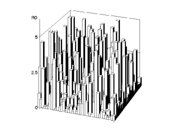
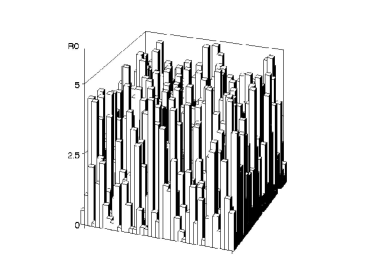
   (a)	(b)

   Figure 4. Two distributions of $R_{0}$ on a $40\times 40$ grid. (a): $26\%$ of the sites are sources; (b): $50\%$ of the sites are sources.

2. In the second case, see Fig. 5 (right), the distribution of $R_{0}$ is as in Fig. 4b. Now the sources represent half of the sites. The eigenvalue $\lambda_{0}=4.30$ is positive. Numerically, we observe the positive infected solution $V_{i}$ of (2.3). Note that $V_{i}$ is smoothly structured in space although $R_{0}$ is not. We also represent $T_{i}$ according to Formula (2.7).

   

   Figure 5. Densities of virus $V$ (top) and target cells $T$ (bottom). Left: $R_{0}$ as in Fig. 4a, $\lambda_{0}<0$ (no infection). Right: $R_{0}$ as in Fig. 4b, $\lambda_{0}>0$ (infection). Here $d_{V}=1,~{}\ell=1,~{}N=40$.

3. Study of the dynamical system

We recall the evolution problem for the virus dynamics:

$$T_{t}=\alpha-\gamma VT-\mu_{T}T,$$ (3.1a)

$$I_{t}=\gamma VT-\mu_{I}I,$$ (3.1b)

$$V_{t}=N\mu_{I}I-\mu_{V}V+d_{V}\Delta V,$$ (3.1c)

set in $\Omega_{\ell}$ with periodic boundary conditions. We consider (3.1a)-(3.1c) as a dynamical system ${\mathscr{S}}(t)$, which has two equilibria: the non-infected trivial solution $(T_{u},I_{u},V_{u})$ and the infected, positive solution $(T_{i},I_{i},V_{i})$, the latter for $\lambda_{0}>0$ only. At first, we prove that the non-infected solution is stable for $\lambda_{0}<0$ and unstable for $\lambda_{0}>0$. By stable we mean asymptotically stable. For $\lambda_{0}>0$ the instability of $(T_{u},I_{u},V_{u})$ does not usually imply the stability of $(T_{i},I_{i},V_{i})$. Our aim is to prove the existence of a universal (or maximal) attractor which attracts all the orbits (see e.g., [25]). Since System (3.1a)-(3.1c) is only partly dissipative, we will use a result of Marion [16]. Some special cases where the stability of the infected solution is granted will be discussed afterwards.

Let us introduce the following notations: ${\mathscr{D}}$ is the domain in ${\mathbb{R}}^{3}$ defined by:

$${\mathscr{D}}=\{(x,y,z)\in{\mathbb{R}}^{3}:0\leq x+y\leq M_{1},\;0\leq z\leq M_{2}\},$$

where $M_{1}$, $M_{2}$ are positive constants which will be fixed throughout the proof of the next theorem. We also set for ${\bf u}:=(u_{1},u_{2},u_{3})$:

$${\bf H}=\{{\bf u}\in(L^{2})^{3}:\ {\bf u}(x)\in{\mathscr{D}}\;\,\mbox{for a.e.}\;x\in\Omega_{\ell}\},\quad{\bf V}=L^{2}\times L^{2}\times H_{\sharp}^{1}.$$

Our main result is the following theorem.

Theorem 3.1.

The following properties are met:

1. if $\lambda_{0}<0$, the trivial non-infected solution to Problem (3.1a)-(3.1c) is stable;

2. if $\lambda_{0}>0$, the trivial non-infected solution to Problem (3.1a)-(3.1c) is unstable;

3. if $\lambda_{0}>0$ and $\alpha\in W^{1,\infty}(\Omega_{\ell})$, the dynamical system ${\mathscr{S}}(t)$ associated with (3.1a)-(3.1c) possesses a universal attractor that is connected in H.

3.1. Proof of (i)

We begin the proof observing that the linearization (around $(T_{u},I_{u},V_{u})$) of Problem (3.1a)-(3.1c) is associated with the linear operator ${\mathscr{L}}_{u}$ defined by

$${\mathscr{L}}_{u}=\begin{pmatrix}-\mu_{T}Id&0&-\displaystyle\frac{\gamma\alpha}{\mu_{T}}Id\\[9.95845pt] 0&-\mu_{I}Id&\displaystyle\frac{\gamma\alpha}{\mu_{T}}Id\\[9.95845pt] 0&N\mu_{I}Id&d_{V}\Delta-\mu_{V}Id\end{pmatrix}.$$

Its realization $L_{u}$ in $(L^{2})^{3}$ with domain $D(L_{u})=L^{2}\times L^{2}\times H^{2}_{\sharp}$ generates an analytic strongly continuous semigroup. Indeed, $L_{u}$ is a bounded perturbation of the diagonal operator

$$\begin{pmatrix}-\mu_{T}Id&0&0\\[9.95845pt] 0&-\mu_{I}Id&0\\[9.95845pt] 0&0&d_{V}\Delta-\mu_{V}Id\end{pmatrix},$$

defined in $L^{2}\times L^{2}\times H^{2}_{\sharp}$, which is clearly sectorial since all its entries are. Hence, we can apply [15, Prop. 2.4.1(i)] and conclude that $L_{u}$ is sectorial. Since $H^{2}_{\sharp}$ is dense in $L^{2}$, the associated analytic semigroup is strongly continuous.

Let us prove that all the elements of the spectrum of $L_{u}$ have negative real part. In view of the linearized stability principle (see e.g., [10, Chapt. 5, Cor. 5.1.6]) this will imply that the trivial non-infected solution to Problem (3.1a)-(3.1c) is stable.

To study the spectrum of the operator $L_{u}$, we fix ${\bf f}=(f_{1},f_{2},f_{3})\in(L^{2})^{3}$ and consider the resolvent system

$$(\lambda+\mu_{T})\varphi_{1}+\frac{\alpha\gamma}{\mu_{T}}\varphi_{3}=f_{1},$$ (3.2a)

$$(\lambda+\mu_{I})\varphi_{2}-\frac{\alpha\gamma}{\mu_{T}}\varphi_{3}=f_{2},$$ (3.2b)

$$(\lambda+\mu_{V})\varphi_{3}-d_{V}\Delta\varphi_{3}-N\mu_{I}\varphi_{2}=f_{3},$$ (3.2c)

where we look for a triplet of functions $\varphi_{1},\varphi_{2}\in L^{2}$ and $\varphi_{3}\in H^{2}_{\sharp}$. Suppose that $\lambda$ differs from both $-\mu_{I}$ and $-\mu_{T}$ (which belong to the essential spectrum). Then, we can use equations (3.2a) and (3.2b) to make $\varphi_{1}$ and $\varphi_{2}$ explicit in terms of $\varphi_{3}$. In particular, replacing the expression of $\varphi_{2}$ in terms of $\varphi_{3}$ into (3.2c) and using the very definition of the function $R_{0}$ (see (1.5)), we can transform Problem (3.2a)-(3.2c) into the equivalent equation for $\varphi_{3}$ only:

$$(\lambda+\mu_{V})\varphi_{3}-d_{V}\Delta\varphi_{3}-\frac{\mu_{I}\mu_{V}}{\lambda+\mu_{I}}R_{0}\varphi_{3}=\frac{N\mu_{I}}{\lambda+\mu_{I}}f_{2}+f_{3}.$$ (3.3)

Adding and subtracting $-\mu_{V}R_{0}$ from the left-hand side of (3.3), we can rewrite the equation (3.3) into the equivalent form:

$$(\lambda+\mu_{V})\varphi_{3}-d_{V}\Delta\varphi_{3}-\mu_{V}R_{0}\varphi_{3}+\mu_{V}R_{0}\frac{\lambda}{\lambda+\mu_{I}}\varphi_{3}=\frac{N\mu_{I}}{\lambda+\mu_{I}}f_{2}+f_{3}.$$ (3.4)

Note that, for any $\lambda\in{\mathbb{C}}$, the operator $A_{\lambda}$ defined by the left-hand side of (3.4) has compact resolvent. Hence, its spectrum consists of eigenvalues only. We are going to prove that, for $\lambda\in{\mathbb{C}}$ with non-negative real part, $0$ is not an eigenvalue of $A_{\lambda}$. For this purpose, we observe that $-\lambda_{0}$ can be equivalently characterized as the infimum of the ratio

$$\frac{d_{V}\int_{\Omega_{\ell}}|\nabla\psi|^{2}dx+\mu_{V}\int_{\Omega_{\ell}}(1-R_{0})|\psi|^{2}dx}{\int_{\Omega_{\ell}}|\psi|^{2}dx}$$

when $\psi$ runs in the set of all the complex-valued functions $\psi=\psi_{1}+i\psi_{2}$, with $\psi_{1},\psi_{2}\in H^{1}_{\sharp}$. This shows, in particular, that

$$-\lambda_{0}\int_{\Omega_{\ell}}|\psi|^{2}dx\leq d_{V}\int_{\Omega_{\ell}}|\nabla\psi|^{2}dx+\mu_{V}\int_{\Omega_{\ell}}(1-R_{0})|\psi|^{2}dx,$$ (3.5)

for any function $\psi$ as above.

Let now $\varphi_{3}$ be a complex-valued solution to (3.4). Multiplying both the sides of such an equation by the conjugate of $\varphi_{3}$ and integrating by parts, we easily see that

$$(\lambda +\mu_{V})\int_{\Omega_{\ell}}|\varphi_{3}|^{2}dx+d_{V}\int_{\Omega_{\ell}}|\nabla\varphi_{3}|^{2}dx-\mu_{V}\int_{\Omega_{\ell}}R_{0}|\varphi_{3}|^{2}dx$$

$$+\frac{\mu_{V}\lambda}{\lambda+\mu_{I}}\int_{\Omega_{\ell}}R_{0}|\varphi_{3}|^{2}dx=0.$$ (3.6)

Taking the real part of both the sides of (3.6) and using (3.5), we obtain

$$({\rm Re}\lambda+\mu_{V})\int_{\Omega_{\ell}}|\varphi_{3}|^{2}dx-\lambda_{0}\int_{\Omega_{\ell}}|\varphi_{3}|^{2}dx+\mu_{V}\frac{|\lambda|^{2}+\mu_{I}{\rm Re}\lambda}{|\lambda+\mu_{I}|^{2}}\int_{\Omega_{\ell}}|\varphi_{3}|^{2}dx\leq 0.$$

Since, by assumptions, $\lambda_{0}<0$ and $R_{0}$ is a positive-valued function, the only solution to the previous inequality, when ${\rm Re}\lambda\geq 0$, is the trivial function $\varphi_{3}\equiv 0$. Hence, for these values of $\lambda$, $0$ is not an eigenvalue of the operator $A_{\lambda}$, i.e., any $\lambda$ with non-negative real part belongs to the resolvent set of the operator $L_{u}$.

3.2. Proof of (ii)

Again in view of the linearized stability principle, to prove the instability of non-infected solution $(T_{u},I_{u},V_{u})$ we can limit ourselves to showing that $L_{u}$ admits a positive eigenvalue. Hence, we are led to the study of Problem (3.2a)-(3.2c) with $f_{1}\equiv f_{2}\equiv f_{3}\equiv 0$. Since the parameters $\mu_{T}$, $\mu_{I}$ and $\mu_{V}$ are all positive and we are looking for positive eigenvalues $\lambda$, we can limit ourselves, as in the proof of (i), to studying the equation

$$d_{V}\Delta\varphi_{3}+\mu_{V}\left(\frac{\mu_{I}R_{0}}{\lambda+\mu_{I}}-1\right)\varphi_{3}=\lambda\varphi_{3}.$$

For any $s\geq 0$, let us consider the operator $d_{V}\Delta+\mu_{V}\left(\frac{\mu_{I}R_{0}}{s+\mu_{I}}-1\right)Id$ defined in $H^{2}_{\sharp}$. By Theorem 2.1 its spectrum consists of eigenvalues only, and the largest one is given by the following formula:

$$-\lambda(s)=\inf_{\psi\in H^{1}_{\sharp},\psi\not\equiv 0}\left\{\frac{d_{V}\int_{\Omega_{\ell}}|\nabla\psi|^{2}dx+\mu_{V}\int_{\Omega_{\ell}}\left(1-\frac{\mu_{I}R_{0}}{s+\mu_{I}}\right)\psi^{2}dx}{\int_{\Omega_{\ell}}\psi^{2}dx}\right\}.$$

As it is immediately seen, $\lambda(0)=\lambda_{0}$. Moreover, since the function $s\mapsto\frac{\mu_{I}R_{0}}{s+\mu_{I}}$ is continuous, decreasing in $[0,+\infty)$ and it tends to $0$ as $s\to+\infty$, the function $s\mapsto\lambda(s)$ is continuous, decreasing and tends to

$$\lambda(+\infty)=-\inf_{\psi\in H^{1}_{\sharp},\psi\not\equiv 0}\left\{\frac{d_{V}\int_{\Omega_{\ell}}|\nabla\psi|^{2}dx+\mu_{V}\int_{\Omega_{\ell}}\psi^{2}dx}{\int_{\Omega_{\ell}}\psi^{2}dx}\right\},$$

as $s\to+\infty$, i.e., it converges to the largest eigenvalue of the operator $d_{V}\Delta-\mu_{V}Id$, which clearly is $-\mu_{V}$. Now, since $s\mapsto\lambda(s)$ is a decreasing continuous function mapping $[0,+\infty)$ into $[-\mu_{V},\mu_{V}^{-1}\lambda_{0}]$, it is immediate to check that the fixed point equation $s=\lambda(s)$ has a positive solution. Of course, this fixed point is the positive eigenvalue of the operator $L_{u}$ we were looking for. This accomplishes the proof.

3.3. Proof of (iii)

Let us show that [16, Thm. 5.1] applies. In this respect the assumption $\alpha\in W^{1,\infty}(\Omega_{\ell})$ is enough. To avoid conflict with notations, throughout the proof, $T$ denotes time as usual, whereas the triplet $(T,I,V)$ is denoted by $(u_{1},u_{2},u_{3})$. We split the proof into several steps.

Step 1. Here, we prove that, for any ${\bf u_{0}}:=(u_{0,1},u_{0,2},u_{0,3})\in(L^{2})^{3}$, the Cauchy problem

$$\left\{\begin{array}[]{ll}D_{t}u_{1}(t,\cdot)=-\mu_{T}u_{1}(t,\cdot)-\gamma u_{1}(t,\cdot)u_{3}(t,\cdot)+\alpha(\cdot),&t>0,\\[5.69054pt] D_{t}u_{2}(t,\cdot)=-\mu_{I}u_{2}(t,\cdot)+\gamma u_{1}(t,\cdot)|u_{3}(t,\cdot)|,&t>0,\\[5.69054pt] D_{t}u_{3}(t,\cdot)=\Delta u_{3}(t,\cdot)-\mu_{V}u_{3}(t,\cdot)+N\mu_{I}u_{2}(t,\cdot),&t>0,\\[5.69054pt] u_{i}(0,\cdot)=u_{0,i},\;\;i=1,2,3,\end{array}\right.$$ (3.7)

Problem (3.7) admits a unique classical solution defined in some time domain $(0,T_{*})$. Here, by classical solution, we mean a vector valued function ${\bf u}$ such that $u_{1},u_{2}\in C^{1}((0,T_{*});L^{2})\cap C([0,T_{*});L^{2})$ and $u_{3}\in C([0,T_{*});L^{2})\cap C^{1}((0,T_{*});L^{2})\cap C((0,T_{*});H^{2}_{\sharp})$.

Problem (3.7) is semilinear with a nonlinear term which is a continuous function from $L^{2}\times L^{2}\times D_{\Delta_{2}}(\beta,2)$ into $L^{2}\times L^{2}\times L^{2}$ for any $\beta\in(1/2,1)$. Here, $D_{\Delta_{2}}(\beta,2)$ is the interpolation space of order $(\beta,2)$ between $L^{2}$ and the domain of the realization $\Delta_{2}$ of the Laplacian with periodic boundary conditions in $L^{2}$ (i.e., $D(\Delta_{2})=H^{2}_{\sharp}$). Hence, $D_{\Delta_{2}}(\beta,2)=(L^{2},H^{2}_{\sharp})_{\beta,2}$ and this latter space coincides with $H^{2\beta}_{\sharp}$, which continuously embeds into the space $C_{\sharp}$ of all continuous and periodic (with period $\ell$ in each variable) functions (see e.g., [9, Thm. 1.4.4.1]).

To prove the existence of a classical solution to Problem (3.7), let us fix $\beta\in(1/2,1)$ and introduce, for any $T>0$, the space $C_{\beta}(T)$ consisting of all functions $v:(0,T)\to D_{\Delta_{2}}(\beta,\infty)$ such that $\|v\|_{C_{\beta}(T)}:=\sup_{t\in(0,T]}\|t^{\beta}v(t,\cdot)\|_{D_{\Delta_{2}}(\beta,\infty)}<+\infty$. Clearly, $C_{\beta}(T)$ is a Banach space when endowed with the above norm. Moreover, $D_{\Delta_{2}}(\beta,\infty)$ is continuously embedded into $D_{\Delta_{2}}(\beta-\varepsilon,2)$ for any $\varepsilon\in(0,\beta)$. We now fix $\varepsilon$ small enough such that $\theta=\beta-\varepsilon>1/2$. From the above results, it is immediate to infer that $C_{\beta}(T)$ is embedded into the set of all continuous functions $f:(0,T]\times\overline{\Omega}_{\ell}\to{\mathbb{R}}$ and there exists a positive constant $C_{1}$, independent of $T$, such that

$$\sup_{t\in(0,T]}t^{\theta}\|f(t,\cdot)\|_{\infty}\leq C_{1}\|f\|_{C_{\beta}(T)}.$$ (3.8)

Let us solve the Cauchy problem for $u_{1}$, taking $u_{3}$ as a parameter. The (unique) solution to such a problem in $C^{1}((0,T];L^{2})\cap C([0,T];L^{2})$ is the function $u_{1}$ defined by

$$u_{1}(t,\cdot)= \exp\left(-\mu_{T}t-\gamma\int_{0}^{t}u_{3}(s,\cdot)ds\right)u_{0,1}$$

$$+\alpha(\cdot)\int_{0}^{t}\exp\left(-\mu_{T}(t-s)-\gamma\int_{s}^{t}u_{3}(r,\cdot)dr\right)ds,$$ (3.9)

for any $t\in(0,T]$. If $u_{0,1}$ is bounded and continuous in $\Omega_{\ell}$ this result is straightforward. In the general case, we approximate $u_{0,1}\in L^{2}$ by a sequence of smooth functions $u_{0,1}^{(n)}$. It is immediate to check that the function $u_{1}^{(n)}$ defined by (3.9), with $u_{0,1}^{(n)}$ instead of $u_{0,1}$, converges to the function $u_{1}$ in $\eqref{op-Lambda-1}$ in $C([0,T];L^{2})$, by dominated convergence. Similarly, $D_{t}u_{1}^{(n)}$ converges to $D_{t}u_{1}$ in $C([\varepsilon,T-\varepsilon];L^{2})$ for any $\varepsilon>0$. It follows that the function $u_{1}$ in (3.9) is a solution to the Cauchy problem for $u_{1}$ also in the case when $u_{0,1}$ is in $L^{2}$.

Let us now denote by $\Lambda_{1}$ the operator defined in $C_{\beta}(T)$ by the right-hand side of (3.9). A very easy computation shows that $\Lambda_{1}$ maps $C_{\beta}(T)$ into $C^{1-\theta}([0,T];L^{2})$. Moreover,

$$\|\Lambda_{1}(v)\|_{C([0,T];L^{2})}\leq\exp\left(\frac{C_{1}}{1-\theta}\gamma T^{1-\theta}\|v\|_{C_{\beta}(T)}\right)\left(\|u_{0,1}\|_{L^{2}}+T\|\alpha\|_{L^{2}}\right),$$ (3.10a)

$$\|\Lambda_{1}(v)-\Lambda_{1}(w)\|_{C([0,T];L^{2})}$$

$$\leq \exp\left(\frac{C_{1}}{1-\theta}\gamma T^{1-\theta}\max(\|v\|_{C_{\alpha}(T)},\|w\|_{C_{\beta}(T)})\right)$$

$$\qquad\qquad\qquad\times\left(1+\frac{C_{1}}{(1-\theta)(2-\theta)}\gamma T^{2-\theta}\|\beta\|_{L^{2}}\right)\|w-v\|_{C_{\beta}(T)}.$$ (3.10b)

We now consider the equation for $u_{2}$. Replacing $u_{1}=\Lambda_{1}(u_{3})$ in the right-hand side of this equation and using the same argument as above, we easily see that the (unique) solution in $C([0,T];L^{2})\cap C^{1}((0,T];L^{2})$ is the function $u_{2}$ defined by

$$u_{2}(t,\cdot)=e^{-t\mu_{I}}u_{0,2}+\gamma\int_{0}^{t}e^{-\mu_{I}(t-s)}|u_{3}(s,\cdot)|(\Lambda_{1}(u_{3}))(s,\cdot)ds,\qquad\;\,t\in[0,T].$$ (3.11)

Let us denote by $\Lambda_{2}$ the operator defined in $C_{\beta}(T)$ by the right-hand side of (3.11). Taking (3.8), (3.10a) and (3.10b) into account, one can easily show that

$$\|\Lambda_{2}(v)\|_{C([0,T];L^{2})}\leq\|u_{0,2}\|_{L^{2}}+\frac{C_{1}}{1-\theta}\gamma T^{1-\theta}\|v\|_{C_{\beta}(T)}\left(\|u_{0,1}\|_{L^{2}}+T\|\alpha\|_{L^{2}}\right)$$

$$\qquad\qquad\qquad\qquad\qquad\qquad\qquad\qquad\times\exp\left(\frac{C_{1}}{1-\theta}\gamma T^{1-\theta}\|v\|_{C_{\beta}(T)}\right),$$ (3.12a)

$$\|\Lambda_{2}(v)\|_{C^{1-\theta}([0,T];L^{2})}\leq\left(\frac{1}{\mu_{I}}T^{\theta}+1\right)\|u_{0,2}\|_{L^{2}}$$

$$\qquad\qquad\qquad\qquad+\frac{C_{1}}{1-\theta}\gamma(1+T^{1-\theta})\|v\|_{C_{\beta}(T)}\exp\left(\frac{C_{1}}{1-\theta}\gamma T^{1-\theta}\|v\|_{C_{\beta}(T)}\right)$$

$$\qquad\qquad\qquad\qquad\qquad\qquad\times\left(\|u_{0,1}\|_{L^{2}}+T\|\alpha\|_{L^{2}}\right),$$ (3.12b)

$$\|\Lambda_{2}(w)-\Lambda_{2}(v)\|_{C([0,T];L^{2})}$$

$$\leq \frac{C_{1}}{1-\theta}\gamma T^{1-\theta}\exp\left(\frac{C_{1}}{1-\theta}\gamma T^{1-\theta}\max(\|v\|_{C_{\beta}(T)},\|w\|_{C_{\beta}(T)})\right)\|w-v\|_{C_{\beta}(T)}$$

$$\qquad\times\left\{\|u_{0,1}\|_{L^{2}}+T\|\theta\|_{L^{2}}+\|v\|_{C_{\beta}(T)}\left(1+\frac{C_{1}}{(1-\theta)(2-\theta)}\gamma T^{2-\theta}\|\beta\|_{L^{2}}\right)\right\},$$ (3.12c)

for any $v,w\in C_{\beta}(T)$. Let us now observe that $(u_{1},u_{2},u_{3})$ is a classical solution to Problem (3.7) if and only if $u_{3}$ is a fixed point of the operator $\Gamma$, formally defined by

$$(\Gamma(v))(t,\cdot)=e^{-t\mu_{V}}e^{t\Delta_{2}}u_{0,3}+\int_{0}^{t}e^{-\mu_{V}(t-s)}e^{(t-s)\Delta_{2}}(\Lambda_{2}(v))(s,\cdot)ds,\qquad\,t\in(0,T).$$

We are going to prove that the operator $\Gamma$ is a contraction in ${\mathscr{Y}}_{\beta}(T)=\{u\in C_{\beta}(T):\|u\|_{C_{\beta}(T)}\leq M\}$ provided that $T$ and $M$ are properly chosen. As a first step, let us prove that $\Gamma$ maps ${\mathscr{Y}}_{\beta}(T)$ into itself if $T,M$ are suitably chosen. For this purpose, we set

$$K:=\sup_{t>0}\|t^{\beta}e^{t\Delta_{2}}\|_{D_{\Delta_{2}}(\beta,\infty)}.$$

Taking (3.12a) into account, we can estimate

$$\|\Gamma (v)\|_{C_{\beta}(T)}\leq K\left\{\|u_{0,3}\|_{L^{2}}+\frac{T}{1-\beta}\|u_{0,2}\|_{L^{2}}\right.$$

$$\left.+\frac{C_{1}M}{(1-\beta)(1-\theta)}\gamma T^{2-\theta}\exp\left(\frac{C_{1}}{1-\theta}\gamma T^{1-\theta}M\right)\left(\|u_{0,1}\|_{C_{\beta}(T)}+T\|\alpha\|_{L^{2}}\right)\right\},$$

for any $v\in{\mathscr{Y}}_{\beta}(T)$. Hence, if we fix $M>K\|u_{0,3}\|_{L^{2}}$, we can then choose $T$ small enough such that $\|\Gamma(v)\|_{C_{\beta}(T)}\leq M$ for any $v\in{\mathscr{Y}}_{\beta}(T)$. Moreover, taking (3.12c) into account, we can estimate

$$\|\Gamma(w) -\Gamma(v)\|_{C_{\beta}(T)}\leq\frac{K}{1-\beta}T\|\Lambda_{2}(w)-\Lambda_{2}(v)\|_{C([0,T];L^{2})}$$

$$\leq\frac{KC_{1}}{(1-\beta)(1-\theta)}\gamma T^{2-\theta}\exp\left(\frac{C_{1}}{1-\theta}\gamma T^{1-\theta}M\right)\|w-v\|_{C_{\theta}(T)}$$

$$\qquad\quad\;\times\left\{\|u_{0,1}\|_{L^{2}}+T\|\alpha\|_{L^{2}}+M\left(1+\frac{C_{1}}{(1-\theta)(2-\theta)}\gamma T^{2-\theta}\|\alpha\|_{L^{2}}\right)\right\},$$

for any $v,w\in{\mathscr{Y}}_{\theta}(T)$. This estimate shows that $\Gamma$ is a $1/2$-contraction provided that $T$ is sufficiently small. We can thus apply the Banach fixed point theorem and conclude that there exist $T>0$ and a unique function $u_{3}\in{\mathscr{Y}}_{\beta}(T)$ solving the equation $\Gamma(u_{3})=u_{3}$.

The function $u_{3}$ actually belongs to $C([0,T];L^{2})\cap C^{1}((0,T];L^{2})\cap C((0,T];H^{2}_{\sharp})$. Indeed, by (3.12b), the function $\Lambda_{2}(u_{3})$ is in $C^{1-\beta}([0,T];L^{2})$. Therefore, [15, Thm. 4.3.1(i)] guarantees that the function $\Gamma(u_{3})$ has the claimed regularity properties. Moreover, $D_{t}u_{3}=\Delta u_{3}-\mu_{V}u_{3}+\Lambda_{2}(u_{3})$ in $(0,T]$. As a byproduct, the triplet $(u_{1},u_{2},u_{3})$ is a classical solution to Problem (3.7).

By a classical argument we can extend the solution $(u_{1},u_{2},u_{3})$ to a maximal solution defined in some time domain $[0,T_{*})$. This vector valued function (still denoted by $(u_{1},u_{2},u_{3})$) enjoys the following properties: $u_{1},u_{2}\in C([0,T_{*});L^{2})\cap C^{1}((0,T_{*});L^{2})$, $u_{3}\in C([0,T_{*});L^{2})\cap C^{1}((0,T_{*});L^{2})\cap C((0,T_{*});H^{2}_{\sharp})$.

Step 2. Here, we prove that if ${\bf u}_{0}\geq 0$ (where the inequality is meant componentwise) then the maximal defined solution ${\bf u}$ to Problem (3.7) is non-negative as well in $(0,T_{*})$. Clearly, using formulae (3.9) and (3.11) it is immediate to check that $u_{1}$ and $u_{2}$ are both non-negative whenever $u_{0,1}$ is.

Let us now consider the problem for $u_{3}$, which we rewrite here:

$$\left\{\begin{array}[]{ll}D_{t}u_{3}(t,\cdot)=\Delta u_{3}(t,\cdot)-\mu_{V}u_{3}(t,\cdot)+N\mu_{I}u_{2}(t,\cdot),&t\in(0,T_{*}),\\[5.69054pt] u_{3}(0,\cdot)=u_{0,3}.\end{array}\right.$$ (3.13)

The heat semigroup is positive in $C_{\sharp}$ by the maximum principle. Since the heat semigroup in $C_{\sharp}$ is the restriction to $C_{\sharp}$ of the heat semigroup $\{e^{t\Delta_{2}}\}$ in $L^{2}$, by density it follows that $\{e^{t\Delta_{2}}\}$ is non-negative as well. This is enough for our aims. Indeed, the function $u_{3}$ is given by the variation of constants formula

$$u_{3}(t,\cdot)=e^{t(\Delta_{2}-\mu_{V})}u_{0,3}+N\mu_{I}\int_{0}^{t}e^{(t-s)(\Delta_{2}-\mu_{V})}u_{2}(s,\cdot)ds,\qquad\;\,t\in(0,T_{*}),$$ (3.14)

$u_{0,3}$ and $u_{2}$ being non-negative, the function $u_{3}$ is non-negative as well.

We have so proved that any solution to Problem (3.7), corresponding to an initial datum in the first octant, is confined to the first octant for any $t\in(0,T_{*})$. In such a case we can forget the absolute value in (3.7).

Step 3. Here, we prove that any solution ${\bf u}$ to Problem (3.7), corresponding to an initial datum ${\bf u}_{0}\in{\mathscr{D}}$, exists for any positive time and it stays bounded. Here,

$${\mathscr{D}}=\{(x,y,z)\in{\mathbb{R}}^{3}:0\leq x+y\leq M_{1},\;\,0\leq z\leq M_{2}\},$$

$$M_{1}=\frac{\|\alpha\|_{\infty}}{\min\{\mu_{T},\mu_{I}\}},\qquad M_{2}=\frac{M_{1}N\mu_{I}}{\mu_{V}}\|\alpha\|_{\infty}.$$ (3.15)

For this purpose, it is convenient to introduce the so-called Svab-Zeldovich variable $v=u_{1}+u_{2}$. As it is immediately seen, the function $v$ satisfies the Cauchy problem

$$\left\{\begin{array}[]{ll}D_{t}v(t,\cdot)=\alpha-\mu_{T}u_{1}-\mu_{I}u_{2},&t\in(0,T_{*}),\\[5.69054pt] v(0,\cdot)=u_{0,1}+u_{0,2}.\end{array}\right.$$

Since $u_{1}$ and $u_{2}$ are both positive, then

$$D_{t}v(t,\cdot)\leq\alpha-\min\{\mu_{T},\mu_{I}\}v(t,\cdot):=\alpha-\mu v(t,\cdot)\leq\|\alpha\|_{\infty}-\mu v(t,\cdot),\qquad\,\,t\in(0,T_{*}).$$ (3.17)

Multiplying both the sides of (3.17) by a non-negative function $\varphi\in L^{2}$ and integrating over $\Omega_{\ell}$, one obtains that the function $w(t)=\int_{\Omega_{\ell}}v(t,x)\varphi(x)dx$ is in $C^{1}([0,T_{*}))$ and solves the differential inequality

$$D_{t}w(t)\leq\|\alpha\|_{\infty}\|\varphi\|_{L^{1}(\Omega_{\ell})}-\mu w(t),\qquad\;\,t\in(0,T_{*}).$$

Hence,

$$w(t)\leq e^{-\mu t}\left(\int_{\Omega_{\ell}}v(0,x)\varphi(x)dx+\frac{1}{\mu}(e^{\mu t}-1)\|\alpha\|_{\infty}\int_{\Omega_{\ell}}\varphi(x)dx\right),\qquad\,t\in(0,T_{*}),$$

or, equivalently,

$$\int_{\Omega_{\ell}}\left(v(t,x)-e^{-\mu t}v(0,x)-\frac{1}{\mu}(1-e^{-\mu t})\|\alpha\|_{\infty}\right)\varphi(x)dx\leq 0,\qquad\;\,t\in(0,T_{*}).$$

From this integral inequality, we can infer that

$$v(t,x)\leq e^{-\mu t}v(0,x)+\frac{1}{\mu}(1-e^{-\mu t})\|\alpha\|_{\infty}\leq\frac{1}{\mu}\|\alpha\|_{\infty}=M_{1},$$ (3.18)

for any $t\in[0,T_{*})$ and almost any $x\in\Omega_{\ell}$.

Since $v=u_{1}+u_{2}$ and $u_{1}$ and $u_{2}$ are both non-negative, it follows that $u_{1}$ and $u_{2}$ can be estimated by the right-hand side of (3.18).

Finally, let us consider the function $u_{3}$. From (3.14) and the above results, we can infer that

$$D_{t}u_{3}(t,\cdot)\leq\Delta u_{3}(t,\cdot)-\mu_{V}u_{3}(t,\cdot)+M_{1}N\mu_{I},\qquad t\in(0,T_{*}).$$

Note that the function $\overline{u}_{3}\equiv M_{2}$, with $M_{2}$ being given by (3.15), satisfies the previous inequality. Hence, if $u_{0,3}\leq M_{2}$, then, the solution to Problem (3.13) is bounded from above by $M_{2}$. With the previous choices of $M_{1}$ and $M_{2}$, we see that the solution to Problem (3.7) which corresponds to ${\bf u}_{0}\in{\mathscr{D}}$, stays in ${\mathscr{D}}$ for any $t\in(0,T_{*})$. By virtue of [15, Prop. 7.1.8], ${\bf u}$ can be extended to all the positive times.

Step 4. Here, we show that, for any ${\bf u}_{0}\in{\mathscr{D}}$, the solution ${\bf u}$ that we have determined in the previous steps is, in fact, the unique weak solution to Problem (3.7) which belongs to $L^{2}((0,T);L^{2})\times L^{2}((0,T);L^{2})\times L^{2}((0,T);H^{1}_{\sharp})$ for any $T>0$. Even if the following arguments are standard, for the reader’s convenience we go into details.

As a first step, we observe that, since $u_{1}$, $u_{2}$ and $u_{3}$ are bounded, the weak derivatives $D_{t}u_{1}$ and $D_{t}u_{2}$ are in $L^{\infty}((0,+\infty)\times\Omega_{\ell})=L^{\infty}((0,\infty);L^{\infty}(\Omega_{\ell}))$. Hence, $u_{1}$ and $u_{2}$ are locally Lipschitz continuous in $[0,+\infty)$ with values in $L^{\infty}(\Omega_{\ell})$.

Let us now consider the Cauchy problem for $u_{3}$ (i.e., problem (3.13)). Since $u_{2}$ is Lipschitz continuous in $[0,T]$ with values in $L^{2}$, for any $T>0$, by [15, Thm. 4.3.1(i)], such a Cauchy problem admits a solution which is in $C([0,T];L^{2})\cap C^{1}((0,T];L^{2})\cap C((0,T];H^{2}_{\sharp})$. By the weak maximum principle, the Cauchy problem (3.13) admits a unique weak solution. Hence, $u_{3}\in C([0,T];L^{2})\cap C^{1}((0,T];L^{2})\cap C((0,T];H^{2}_{\sharp})$. Now, we turn back to the equations for $u_{1}$ and $u_{2}$ and conclude that $D_{t}u_{1}$ and $D_{t}u_{2}$ are in $C([0,T];L^{2})$ for any $T>0$, this implying that $u_{1}$ and $u_{2}$ are in $C^{1}([0,T];L^{2})$. Hence, any weak solution to Problem (3.7) with data in ${\mathscr{D}}$ is such that $u_{1},u_{2}\in C^{1}([0,T_{*});L^{2})$ and $u_{3}\in C([0,T_{*});L^{2})\cap C^{1}((0,T_{*});L^{2})\cap C((0,T_{*});H^{2}_{\sharp})$. Since we have proved uniqueness of the solution in this class of functions, uniqueness of the weak solution follows as well.

Since for non-negative solutions the Cauchy problem (3.7) coincides with problem (3.1a)-(3.1c), we have, thus, established the following:

Proposition 3.2.

For every ${\bf u_{0}}\in{\bf H}$, the Cauchy problem (3.7) possesses a unique solution for all time, ${\bf u}(t)\in{\bf H}$ for all $t$, ${\bf u}\in L^{2}(0,T;{\bf V})$ for all $T>0$. The mapping ${\mathscr{S}}(t):={\bf u_{0}}\mapsto{\bf u}(t)$ is continuous in ${\bf H}$. Furthermore, if ${\bf u_{0}}\in{\bf V}$, then $u_{3}\in L^{2}(0,T;H_{\sharp}^{2})$.

Step 3. We are now in a position to apply [16, Thm. 5.1]. The set

$${\mathscr{D}}=\{(x,y,z)\in{\mathbb{R}}^{3}:0\leq x+y\leq M_{1},\;0\leq z\leq M_{2}\},$$

is a positively convex, compact region of ${\mathbb{R}}^{3}$. To meet all the hypotheses of [16, Thm. 5.1], it remains to consider the non-dissipative part of (3.7), i.e. the equations for $u_{1}$ and $u_{2}$ which we rewrite in the compact form:

$$D_{t}\begin{pmatrix}u_{1}\\ u_{2}\end{pmatrix}+\begin{pmatrix}\mu_{T}+\gamma u_{3}&0\\ -\gamma u_{3}&\mu_{I}\end{pmatrix}\begin{pmatrix}u_{1}\\ u_{2}\end{pmatrix}+\begin{pmatrix}\alpha\\ 0\end{pmatrix}:=G(\cdot,u_{3})\begin{pmatrix}u_{1}\\ u_{2}\end{pmatrix}+g(\cdot).$$

Obviously the matrix $G(\cdot,u_{3})$ has positive eigenvalues whenever $u_{3}\geq 0$, which are bounded from below by positive constants. Hence,

$$\langle G(\cdot,u_{3})\xi,\xi\rangle\;\geq\mu_{T}\|\xi\|^{2},$$

for any $\xi\in{\mathbb{R}}^{2}$. Thus, condition (4.6) in [16] is satisfied. The proof of Theorem 3.1 is completed.

4. A gamut of some special cases

4.1. Numerical illustration (evolution)

We continue the discussion of Subsection 2.2 in the framework of the evolution problem (3.1a)-(3.1c). In the first case ($\lambda_{0}<0$), only the non-infected steady state $V_{u}\equiv 0$ exists. We solve (3.1a)-(3.1c) under particular initial conditions: we start the infection at the center of the grid with an inoculum of one viral unit, assuming that $T$ and $I$ are at their uninfected steady state. One observes that the virus vanishes very rapidly and the target cells return to their initial level (see Fig. 6 left) in accordance with the stability of the uninfected equilibrium $V_{u}$. In the second case ($\lambda_{0}>0$), two equilibria exist, $V_{u}$ and $V_{i}$. Starting with the same initial conditions, the virus population grows while the population of target cells decreases. Both of them achieve an equilibrium corresponding to the positive infected solution (see Fig. 6 right).

Figure 6. Dynamics of free virus (top) and target cells (bottom) on a $40\times 40$ grid. Left: $R_{0}$ as in Fig. 4a, $\lambda_{0}<0$ (no infection); right: $R_{0}$ as in Fig. 4b, $\lambda_{0}>0$ (infection). The solid, the long and the short dashed lines depict respectively the dynamics at (10,10), at the site of viral inoculum (20,20) and at a border site (1,1). Here $d_{V}=1,~{}\ell=1$.

We are now going to review some particular cases where the stability of the infected solution is granted.

4.2. Homogeneous environment with diffusion

We consider the case when $\alpha$ is a constant such that $R_{0}$ (see (1.3)) is a constant, as well, greater than $1$, together with $d_{V}>0$ as in [8].

The linearization around $(T_{i},I_{i},V_{i})$ (see (1.2)) of Problem (3.1a)-(3.1c) is associated with the linear operator

$${\mathscr{L}}_{i}=\begin{pmatrix}-\mu_{T}R_{0}Id&0&\displaystyle-\frac{\mu_{V}}{N}Id\\[9.95845pt] \mu_{T}(R_{0}-1)Id&-\mu_{I}Id&\displaystyle\frac{\mu_{V}}{N}Id\\[9.95845pt] 0&N\mu_{I}Id&d_{V}\Delta-\mu_{V}Id\\ \end{pmatrix}.$$

The same arguments as in the proof of Theorem 3.1(i) show that the realization $L_{i}$ of the operator ${\mathscr{L}}_{i}$ in $(L^{2})^{3}$ with domain $D(L_{i})=L^{2}\times L^{2}\times H^{2}_{\sharp}$ generates an analytic strongly continuous semigroup. We are going to determine its spectrum. For this purpose we use the discrete Fourier transform.

We consider the realization $\Delta_{2}$ of the operator $\Delta$ with domain ${H}_{\sharp}^{2}$. Its real eigenvalues can be labeled as a non-increasing sequence $(-\lambda_{k}),~{}k=0,1,\ldots$ Only $\lambda_{0}=0$ is simple, the other eigenvalues being negative such that $-\lambda_{k}\to-\infty$ as $k\to+\infty$.

We claim that the spectrum of the operator $L_{i}$ is given by

$$\sigma(L_{i})=\{-\mu_{I},-\mu_{T}R_{0}\}\cup\bigcup_{k\in{\mathbb{N}}\cup\{0\}}\sigma_{k},$$ (4.1)

where $\sigma_{k}$ is the spectrum of the matrix

$$M_{k}=\begin{pmatrix}-\mu_{T}R_{0}&0&\displaystyle-\frac{\mu_{V}}{N}\\[9.95845pt] \mu_{T}(R_{0}-1)&-\mu_{I}&\displaystyle\frac{\mu_{V}}{N}\\[9.95845pt] 0&N\mu_{I}&-\lambda_{k}d_{V}-\mu_{V}\\ \end{pmatrix}.$$

To check the claim, let us observe that, if a function ${\bf v}=(v_{1},v_{2},v_{3})$ in $L^{2}\times L^{2}\times H^{2}$ solves the resolvent equation $\lambda{\bf u}-L_{i}{\bf u}={\bf f}$, for some $\lambda\in{\mathbb{C}}$ and ${\bf f}=(f_{1},f_{2},f_{3})$ in $(L^{2})^{3}$, then its Fourier coefficients $(v_{1,k},v_{2,k},v_{3,k})$ ($k=0,1,\ldots$) solve the infinitely many equations

$$\begin{pmatrix}\lambda+\mu_{T}R_{0}&0&\displaystyle\frac{\mu_{V}}{N}\\[9.95845pt] -\mu_{T}(R_{0}-1)&\lambda+\mu_{I}&\displaystyle-\frac{\mu_{V}}{N}\\[9.95845pt] 0&-N\mu_{I}&\lambda+\lambda_{k}d_{V}+\mu_{V}\\ \end{pmatrix}\begin{pmatrix}v_{1,k}\\[9.95845pt] v_{2,k}\\[9.95845pt] v_{3,k}\end{pmatrix}=\begin{pmatrix}f_{1,k}\\[9.95845pt] f_{2,k}\\[9.95845pt] f_{3,k}\end{pmatrix},\qquad\;\,k=0,1,\ldots,$$

where $f_{i,k}$ denotes the $k$-th Fourier coefficient of the function $f_{i}$ ($i=1,2,3$). Clearly, any eigenvalue of $M_{k}$ ($k=0,1,\ldots$) is an eigenvalue of $L_{i}$. Therefore,

$$\sigma(L_{i})\supset\bigcup_{k\in{\mathbb{N}}\cup\{0\}}\sigma_{k}.$$

On the other hand, if $\lambda\not\in\sigma_{k}$ for any $k=0,1,\ldots$, then all the coefficients $(v_{1,k},v_{2,k},v_{3,k})$ are uniquely determined through the formulae

$$v_{1,k}= \frac{1}{{\mathscr{P}}_{k}(\lambda)}\Big{\{}[(\lambda+\mu_{I})(\lambda+\lambda_{k}d_{V}+\mu_{V})-\mu_{I}\mu_{V}]f_{1,k}-\mu_{I}\mu_{V}f_{2,k}$$

$$\qquad\qquad-\frac{\mu_{V}}{N}(\lambda+\mu_{I})f_{3,k}\Big{\}},$$

$$v_{2,k}= \frac{1}{{\mathscr{P}}_{k}(\lambda)}\Big{\{}\mu_{T}(R_{0}-1)(\lambda+\lambda_{k}d_{V}+\mu_{V})f_{1,k}+(\lambda+\mu_{T}R_{0})(\lambda+\lambda_{k}d_{V}+\mu_{V})f_{2,k}$$

$$\qquad\qquad+\frac{\mu_{V}}{N}(\mu_{T}+\lambda)f_{3,k}\Big{\}},$$

$$v_{3,k}= \frac{1}{{\mathscr{P}}_{k}(\lambda)}\left\{N\mu_{I}\mu_{T}(R_{0}-1)f_{1,k}+N\mu_{I}(\lambda+\mu_{T}R_{0})f_{2,k}\right.$$

$$\qquad\qquad+\left.(\lambda+\mu_{T}R_{0})(\lambda+\mu_{I})f_{3,k}\right\},$$

where

$${\mathscr{P}}_{k}(\lambda)=\lambda^{3}+b_{k}\lambda^{2}+c_{k}\lambda+d_{k}=0,\quad k=0,1,\ldots$$

and

$$b_{k} =\mu_{T}R_{0}+\mu_{I}+\mu_{V}+d_{V}\lambda_{k},$$

$$c_{k} =\mu_{T}R_{0}(\mu_{I}+\mu_{V})+d_{V}\lambda_{k}(\mu_{T}R_{0}+\mu_{I}),$$

$$d_{k} =\mu_{I}\mu_{V}\mu_{T}(R_{0}-1)+d_{V}\lambda_{k}\mu_{I}\mu_{T}R_{0}.$$

Note that, if $\lambda$ differs from both $-\mu_{I}$ and $-\mu_{T}R_{0}$, then

$${\mathscr{P}}_{k}(\lambda)\sim d_{V}\left\{\lambda^{2}+\lambda(\mu_{T}R_{0}+\mu_{I})+\mu_{I}\mu_{T}R_{0}\right\}\lambda_{k},\qquad\;\,{\rm as}~{}k\to+\infty.$$

Hence, for any $\lambda\notin\{-\mu_{I},-\mu_{T}R_{0}\}\cup\bigcup_{k\in{\mathbb{N}}\cup\{0\}}\sigma_{k}$, it holds that

$$v_{1,k} \sim\frac{\lambda+\mu_{I}}{\lambda^{2}+\lambda(\mu_{T}R_{0}+\mu_{I})+\mu_{I}\mu_{T}R_{0}}f_{1,k},$$

$$v_{2,k} \sim\frac{\mu_{T}(R_{0}-1)f_{1,k}+(\lambda+\mu_{T}R_{0})f_{2,k}}{\lambda^{2}+\lambda(\mu_{T}R_{0}+\mu_{I})+\mu_{I}\mu_{T}R_{0}},$$

$$v_{3,k} \sim\frac{N\mu_{I}\mu_{T}(R_{0}-1)f_{1,k}+N\mu_{I}(\lambda+\mu_{T}R_{0})f_{2,k}+(\lambda+\mu_{T}R_{0})(\lambda+\mu_{I})f_{3,k}}{d_{V}\{\lambda^{2}+\lambda(\mu_{T}R_{0}+\mu_{I})+\mu_{I}\mu_{T}R_{0}\}}\frac{1}{\lambda_{k}},$$

as $k\to+\infty$. It follows that the sequences $\{v_{1,k}\}$, $\{v_{2,k}\}$ and $\{\lambda_{k}v_{3,k}\}$ are in $\ell^{2}$. This shows that the series whose Fourier coefficients are $v_{1,k}$, $v_{2,k}$ and $v_{3,k}$, respectively, converge in $L^{2}$ (the first two ones) and in $H^{2}_{\sharp}$ (the latter one). The inclusion

$$\sigma(L_{i})\subset\{-\mu_{I},-\mu_{T}R_{0}\}\cup\bigcup_{k\in{\mathbb{N}}\cup\{0\}}\sigma_{k}$$

follows. We now observe that a straightforward computation shows that $\lambda=-\mu_{T}R_{0}$ is in the essential spectrum of $L_{i}$. Also $\lambda=-\mu_{I}$ belongs to the essential spectrum of $L_{i}$ and, in the case when $\mu_{I}=\mu_{T}$, it belongs also to the point spectrum. The set equality (4.1) is proved.

Clearly $\sigma_{k}$ has three eigenvalues (counted with their multiplicity), either all real, or one real and two complex conjugates. Routh-Hurwitz criterion enables us to determine whether the elements of $\sigma_{k}$ have negative real parts. The latter holds if and only if $b_{k}$, $d_{k}$ and $b_{k}c_{k}-d_{k}$ are positive, which is clearly true whenever $R_{0}>1$.

Remark 4.1.

As it is easily seen $\sigma_{0}$ is the spectrum of the operator

$$\begin{pmatrix}-\mu_{T}R_{0}Id&0&\displaystyle-\frac{\mu_{V}}{N}Id\\[9.95845pt] \mu_{T}(R_{0}-1)Id&-\mu_{I}Id&\displaystyle\frac{\mu_{V}}{N}Id\\[9.95845pt] 0&N\mu_{I}Id&-\mu_{V}Id\\ \end{pmatrix},$$

which is associated with the linearization at $(T_{i},I_{i},V_{i})$ of Problem (1.1a)-(1.1c). Since, as we have already remarked, the spectrum of $L_{i}$ is the union of the sets $\sigma_{k}$ ($k\in{\mathbb{N}}\cup\{0\}$) and the points $-\mu_{I}$, $-\mu_{T}R_{0}$, the scenario is one of the following:

1. the diffusion does not improve the stability of the solution $(T_{i},I_{i},V_{i})$. Therefore, the stability issue is identical to that of the ODE system ($d_{V}=0$);

2. the diffusion worsen the stability of the solution $(T_{i},I_{i},V_{i})$.

Therefore, we are unable to confirm Funk et al. [8], who pointed out that the presence of a spatial structure enhances population stability with respect to non-spatial models. Only some smoothing effect can be credited to the diffusion.

4.3. Death rates $\mu_{I}\leq\mu_{T}$, $\lambda_{0}>0$

This case leads to a mathematically interesting framework although it has little biological relevance, since $\mu_{I}>\mu_{T}$ in the literature (e.g., $\mu_{T}=0.01,~{}\mu_{I}=0.39$ in [5]). For the latter reason we will not elaborate the case extensively.

Using the Svab-Zeldovich variable $v=u_{1}+u_{2}$ we can transform Problem (3.1a)-(3.1c) into the following equivalent one for the unknowns $u_{1}$, $v$ and $u_{3}$:

$$\left\{\begin{array}[]{ll}D_{t}u_{1}(t,\cdot)=-\mu_{T}u_{1}(t,\cdot)-\gamma u_{1}(t,\cdot)u_{3}(t,\cdot)+\alpha(\cdot),&t>0,\\[5.69054pt] D_{t}v(t,\cdot)=\alpha-\mu_{I}v(t,\cdot)-(\mu_{T}-\mu_{I})u_{1}(t,\cdot),&t>0,\\[5.69054pt] D_{t}u_{3}(t,\cdot)=\Delta u_{3}(t,\cdot)-\mu_{V}u_{3}(t,\cdot)+N\mu_{I}v(t,\cdot)-N\mu_{I}u_{1}(t,\cdot),&t>0,\\[5.69054pt] u_{i}(0,\cdot)=u_{0,i},\;\;i=1,3,\\[5.69054pt] v(0,\cdot)=u_{0,1}+u_{0,2}.\end{array}\right.$$ (4.2)

It is not difficult to see that the mapping $u_{3}\mapsto u_{1}$ is non-increasing, so is the mapping $u_{1}\mapsto v$ thanks to the hypothesis $\mu_{T}-\mu_{I}>0$. Hence, the mapping $u_{3}\mapsto v$ is non-decreasing. Finally, the mapping $u_{3}\mapsto u_{2}=v-u_{1}$ is non-decreasing. Based on these observations, following [19] it is possible to construct two sets of monotone sequences which converge to the solution of (4.2). These sequences start respectively from upper and lower solutions defined as in Section 2, to stay away from the trivial solution. It is well-known that a solution of an evolution problem constructed via such a monotone sequence scheme, with suitable initial conditions between upper and lower solutions, achieves a stable equilibrium (see [19]). Therefore, the infected solution is asymptotically stable. Numerical computations in the phase plan (see Fig. 7) illustrate the difference in the virus dynamics when $\mu_{I}<\mu_{T}$ (monotonicity) and $\mu_{I}>\mu_{T}$ (spirals).

(a) $\mu_{I}>\mu_{T}$

(b) $\mu_{I}<\mu_{T}$

Figure 7. Virus vs. target cells in the phase plane, in the case of infection. Left: mean values. Right: the solid, the long and the short dashed lines depict, respectively, the values at (10,10), at the site of viral inoculum (20,20), and at a border site (1,1). The parameters have the following values: $\gamma=0.001,~{}N=1000,~{}\mu_{T}=0.1,~{}\mu_{V}=10,~{}d_{V}=1,~{}\ell=1$; $\alpha$ varies between $0.1$ and $5.0$; $\mu_{I}=1$ in (a), $\mu_{I}=0.01$ in (b).

4.4. Quasi-steady problem

In this part we assume that $T$ and $I$ are at their equilibrium. In such a case, (3.1a)-(3.1c) reads

$$0=\alpha-\gamma VT-\mu_{T}T,$$

$$0=\gamma VT-\mu_{I}I,$$

$$V_{t}=N\mu_{I}I-\mu_{V}V+d_{V}\Delta V,$$

which is equivalent to the scalar parabolic equation for $V$ only, with periodic boundary conditions:

$$V_{t}=d_{V}\Delta V-\mu_{V}V+\mu_{T}\mu_{V}R_{0}\frac{V}{\gamma V+\mu_{T}}.$$ (4.3)

The latter is the natural evolution problem associated with (2.3). It is clear that (4.3) has the same non-positive equilibria, namely $V_{u}=0$ and $V_{i}>0$, in the case when $\lambda_{0}>0$. The stability of $V_{i}$ can be proved according to [10, Sec. 5.3] by constructing a Lyapunov function.

5. Homogenization

This section is concerned with the case wherein the environment is heterogeneous and is formed of rapidly alternating sinks and sources. For a fixed integer $k$, we imagine that $\overline{\Omega_{\ell}}$ is divided into a network of $k^{2}$ periodic squares $\Omega_{\varepsilon}$, where $\varepsilon=\ell/k$. The heterogenous reproductive ratio $R_{0}$ will depend upon $\varepsilon$, see Fig. 8b. The idea of homogenization is to let $\varepsilon\to 0$ and find the equivalent homogenized medium. Therefore, such a heterogenous environment can be replaced by its homogenized limit for easier computations and analysis.

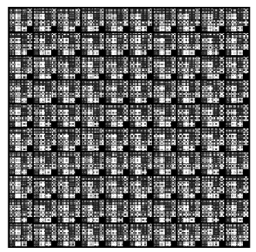
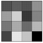
(a)	(b)

Figure 8. Periodic structure with $\ell=1$ (a): $\Omega_{1}$ is divided in a network of $40\times 40$ sites. The sites are pieced together in $4\times 4$ periodic squares $\Omega_{\varepsilon}$ with $\varepsilon=0.1$. (b): zoom of $\Omega_{\varepsilon}$ which contains $16$ sites. The darkness represents the scale of $R_{0}$ on each site (the darker the square, the larger is $R_{0}$).

More precisely, we introduce a normalized periodic function $R_{0}$ as a function of the variable $y=(y_{1},y_{2})$, of period $(1,1)$, and we define:

$$R^{\varepsilon}_{0}(x_{1},x_{2})=R_{0}\left(\frac{x_{1}}{\varepsilon},\frac{x_{2}}{\varepsilon}\right).$$

Remark 5.1.

$x=(x_{1},x_{2})$ is the macroscopic variable while $y=(y_{1},y_{2})$ is the microscopic one.

We consider the problem:

$$d_{V}\Delta V^{\varepsilon}-\mu_{V}V^{\varepsilon}=-\mu_{T}\mu_{V}R^{\varepsilon}_{0}\frac{V^{\varepsilon}}{\gamma V^{\varepsilon}+\mu_{T}},$$ (5.1)

on $\Omega_{\ell}$ with periodic boundary conditions as above. The idea is to find the limiting homogenized equation as $\varepsilon\to 0$. We start with the following lemma:

Lemma 5.2.

Let $R_{0}:{\mathbb{R}}^{2}\to{\mathbb{R}}$ be a periodic $($with period $1$ in each variable$)$, piecewise continuous function. For $x\in{\mathbb{R}}^{2}$ and $\varepsilon>0$, set $R_{0}^{\varepsilon}(x)=R_{0}(\frac{x}{\varepsilon})$. Then, the following properties are met.

1. $R_{0}^{\varepsilon}$ tends to ${\mathscr{M}}_{y}(R_{0})$ as $\varepsilon\to 0$, weakly in $L^{p}_{\rm loc}({\mathbb{R}}^{2})$ for any $p\geq 1$;

2. For any $\varepsilon>0$, set

   $$-\lambda_{0}^{\varepsilon}=\inf_{\psi\in{H^{1}_{\sharp}},\psi\not\equiv 0}\left\{\frac{d_{V}\int_{\Omega_{\ell}}|\nabla\psi|^{2}dx+\mu_{V}\int_{\Omega_{\ell}}(1-R_{0}^{\varepsilon})\psi^{2}dx}{\int_{\Omega_{\ell}}\psi^{2}dx}\right\}.$$ (5.2)

   Then, $\lambda_{0}^{\varepsilon}\to\mu_{V}({\mathscr{M}}_{y}(R_{0})-1)$ as $\varepsilon\to 0$.

Proof.

Property $(i)$ follows straightforwardly from e.g., [12, p. 5]. Thanks to $(i)$, one can take the limit as $\varepsilon\to 0$ in the right-hand side of (5.2) and show that $\lambda_{0}^{\varepsilon}$ tends to the largest eigenvalue of

$$d_{V}\Delta-\mu_{V}(1-{\mathscr{M}}_{y}(R_{0}))Id,$$

on $\Omega_{\ell}$ with periodic boundary conditions. Let us prove this claim. As a first step, we observe that there exist two constants $C_{1}$ and $C_{2}$ such that $C_{1}\leq\lambda_{0}^{\varepsilon}\leq C_{2}$, since the function $R_{0}^{\varepsilon}$ is bounded.

Next, $\lambda_{0}^{\varepsilon}$ is the largest eigenvalue of the Sturm-Liouville eigenvalue problem

$$d_{V}\Delta\psi-\mu_{V}(1-R_{0}^{\varepsilon})\psi=\lambda\psi,$$

with periodic boundary conditions we documented in Theorem 2.1, associated with the eigenfunction $\psi^{\varepsilon}$. We may assume that $\int_{\Omega_{\ell}}(\psi^{\varepsilon})^{2}dx=1$. As we pointed it out in Theorem 2.1, $\psi^{\varepsilon}$ does not change sign.

It is clear that $\psi^{\varepsilon}$ is bounded in $H_{\sharp}^{2}$. Then, there exists an infinitesimal sequence $\{\varepsilon_{n}\}$ such that $\lambda_{0}^{\varepsilon_{n}}\to\lambda_{0}^{0}$, $\psi^{\varepsilon_{n}}\to\psi^{0}$ weakly in $H_{\sharp}^{2}$, strongly in $H_{\sharp}^{2-\eta}$ and (hence) uniformly in ${\overline{\Omega}_{\ell}}$. Note that $\int_{\Omega_{\ell}}(\psi^{0})^{2}dx=1$ and $\psi^{0}$ does not change sign.

Since

$$d_{V}\Delta\psi^{\varepsilon_{n}}-\mu_{V}(1-R_{0}^{\varepsilon_{n}})\psi^{\varepsilon_{n}}=\lambda^{\varepsilon_{n}}\psi^{\varepsilon_{n}},$$

it is not to difficult to pass to the limit in the above equation as $n\to+\infty$ in the distributional sense and see that

$$d_{V}\Delta\psi^{0}-\mu_{V}(1-{\mathscr{M}}_{y}(R_{0}))\psi^{0}=\lambda^{0}_{0}\psi^{0},$$ (5.3)

with periodic boundary conditions. Therefore, $\lambda_{0}^{0}$ is an eigenvalue of the operator $d_{V}\Delta-\mu_{V}(1-R_{0}^{\varepsilon})Id$, associated with the eigenfunction $\psi^{0}$. Since $\psi^{0}$ does not change sign, $\lambda^{0}_{0}$ is the largest eigenvalue of (5.3). Obviously, $\psi^{0}$ is a constant, hence $\lambda^{0}_{0}$ is explicit. Finally, checking that all the sequence $\lambda_{0}^{\varepsilon}$ converges to $\lambda_{0}^{0}$, as $\varepsilon\to 0$, is an easy task. ∎

Next, we prove the following result.

Theorem 5.3.

Assume that ${\mathscr{M}}_{y}(R_{0})>1$. Then, there exists $\varepsilon_{0}$ such that, for any $\varepsilon\in(0,\varepsilon_{0}]$, the equation (5.1) has a positive solution $V^{\varepsilon}\in H^{2}_{\sharp}$. As $\varepsilon\to 0$, $V^{\varepsilon}$ tends to

$$V^{0}=\frac{\mu_{T}}{\gamma}({\mathscr{M}}_{y}(R_{0})-1),$$

in $H^{1}_{\sharp}$ and uniformly in $\overline{\Omega_{\ell}}$.

Proof.

As a first step, we observe that, since ${\mathscr{M}}_{y}(R_{0})>1$, from Lemma 5.2(ii) it follows that there exist $\delta,~{}\varepsilon_{0}>0$ such that $\lambda_{0}^{\varepsilon}>\delta$ for $\varepsilon\in(0,\varepsilon_{0}]$, and (5.1) has a unique positive solution $V^{\varepsilon}$. Clearly, $\Delta V^{\varepsilon}$ is bounded in $L^{\infty}(\Omega_{\ell})$ and this implies that $V^{\varepsilon}$ is bounded in $H^{2}_{\sharp}$. Arguing as in the proof of Lemma 5.2, one can extract an infinitesimal sequence $\{\varepsilon_{n}\}$ such that $V^{\varepsilon_{n}}$ converges strongly in $H^{2-\eta}$ to a limit $V^{0}\in H^{2}_{\sharp}$, which verifies the equation

$$d_{V}\Delta V^{0}-\mu_{V}V^{0}=-\mu_{T}\mu_{V}{\mathscr{M}}_{y}(R_{0})\frac{V^{0}}{\gamma V^{0}+\mu_{T}}.$$ (5.4)

Because of the periodic boundary conditions, Equation (5.4) has only constant solutions. Therefore,

$$-\mu_{V}V^{0}=-\mu_{T}\mu_{V}{\mathscr{M}}_{y}(R_{0})\frac{V^{0}}{\gamma V^{0}+\mu_{T}},$$

and it only remains to prove that $V^{0}$ is not the trivial solution. With obvious notations, we recall (see the proof of Theorem 2.4) that $V^{\varepsilon}\geq\underline{v}_{0}^{\varepsilon}=c^{\varepsilon}\varphi_{0}^{\varepsilon}$ where $\varphi_{0}^{\varepsilon}$ is the positive eigenfunction associated with the largest eigenvalue $\lambda_{0}^{\varepsilon}$ and

$$c^{\varepsilon}=\min\left\{\frac{\lambda_{0}^{\varepsilon}}{\gamma\mu_{V}{\mathscr{R}}},\frac{\mu_{T}({\mathscr{R}}-1)}{\gamma}\right\}\geq\min\left\{\frac{\delta}{\gamma\mu_{V}{\mathscr{R}}},\frac{\mu_{T}({\mathscr{R}}-1)}{\gamma}\right\}.$$

Since $\max\varphi_{0}^{\varepsilon}=1$, it is clear that $V^{\varepsilon}$ remains bounded away from $0$ whenever $\varepsilon\leq\varepsilon_{0}$.

Finally, checking that $V^{\varepsilon}$ itself converges to $V^{0}$ as $\varepsilon\to 0$ is immediate. This concludes the proof. ∎

5.1. Numerical illustration (homogenization)

We consider a model where $R_{0}$ is as in Fig. 8, taking its values on the elementary $4\times 4$ grid (b) as in Tab. 1.

$j$	$R_{0}(1,j)$	$R_{0}(2,j)$	$R_{0}(3,j)$	$R_{0}(4,j)$
$1$	$1.60$$0$	$1.41$$0$E$-4$	$1.55$$0$	$0.819$
$2$	$0.800$	$0.165$E$-4$	$2.59$$0$	$0.872$
$3$	$1.20$$0$	$0.489$E$-4$	$1.37$$0$	$0.453$
$4$	$2.09$$0$	$4.25$E$-4$$0$	$0.270$	$2.80$$0$

Table 1. Values of $R_{0}(i,j)$, $i,j=1,\ldots,4$, on $\Omega_{\varepsilon}$ as in Fig. 8b, to be viewed as a $4\times 4$ matrix.

It is easy to compute the mean value ${\mathscr{M}}_{y}(R_{0})=1.16$ and the homogenized viral density $V^{0}=16.1$. Fig. 9 shows how the virus $V^{\varepsilon}$ at $\varepsilon=0.1$ (left) oscillates slightly around its homogenized limit $V^{0}$ (right).

Figure 9. $V^{\varepsilon}$ (left) vs. $V^{0}$ (right). The grid and parameters are as in Fig. 8 and Tab. 1; $\varepsilon=0.1,~{}d_{V}=1,~{}\ell=1$.

Appendix A Proof of Theorem 2.1

Proof.

It is well known that the realization $\Delta_{2}$ of the Laplacian in $L^{2}$, with domain $H^{2}_{\sharp}$, is a sectorial operator. Since ${\mathscr{A}}$, is a bounded perturbation of the Laplacian, ${\mathscr{A}}$ is sectorial as well, and, hence, its spectrum is not empty. Let us fix $\lambda_{0}\in\rho({\mathscr{A}})\cap(\mu_{\infty},+\infty)$ such that $[\lambda_{0},+\infty)$ is in the resolvent set of $T$. Here, by $\mu_{\infty}$ we denote the sup-norm of the function $\mu$. The operator ${\mathscr{A}}_{0}:={\mathscr{A}}-\lambda_{0}I$ turns out to be invertible and its resolvent set contains $[0,+\infty)$. Since the operator $T_{0}^{-1}$ is continuous from $L^{2}$ into $H^{2}_{\sharp}$, it is continuous, in particular, from $H^{1}_{\sharp}$ into itself, when this latter space is endowed with the inner product

$$\langle v,w\rangle =d\int_{\Omega_{\ell}}(D_{x_{1}}vD_{x_{1}}w+D_{x_{2}}vD_{x_{2}}w)dx+\int_{\Omega_{\ell}}(\mu+\lambda_{0})vwdx$$

$$:=d\int_{\Omega_{\ell}}\nabla v\cdot\nabla wdx+\int_{\Omega_{\ell}}(\mu+\lambda_{0})vwdx,$$

which is equivalent to the Euclidean inner product of $H^{1}$. Since $H^{2}_{\sharp}$ is compactly embedded into $H^{1}_{\sharp}$ (see e.g., [1, Thm. 3.7]), the operator ${\mathscr{A}}_{0}^{-1}$ is compact from $H^{1}_{\sharp}$ into itself. Moreover, ${\mathscr{A}}_{0}^{-1}$ is self-adjoint in $H^{1}_{\sharp}$. Indeed,

$$\langle{\mathscr{A}}_{0}^{-1}u,v\rangle= d\int_{\Omega_{\ell}}\nabla{\mathscr{A}}_{0}^{-1}u\cdot\nabla vdx+\int_{\Omega_{\ell}}(\mu+\lambda_{0}){\mathscr{A}}_{0}^{-1}u\,vdx$$

$$= -d\int_{\Omega_{\ell}}\Delta{\mathscr{A}}_{0}^{-1}u\,vdx+\int_{\Omega_{\ell}}(\mu+\lambda_{0}){\mathscr{A}}_{0}^{-1}u\,vdx$$

$$= -\int_{\Omega_{\ell}}uvdx,$$ (A.1)

for any $u,v\in L^{2}$. Now, from the general theory of self-adjoint compact operators, it follows that the spectrum of ${\mathscr{A}}_{0}^{-1}$ consists of a sequence of real eigenvalues which converges to $0$. As a byproduct, the spectrum of ${\mathscr{A}}_{0}$ consists of a sequence of eigenvalues diverging to $-\infty$. More precisely, $\sigma({\mathscr{A}}_{0})\subset(-\infty,0)$ and $\lambda\in\sigma({\mathscr{A}}_{0})$ if and only if $\lambda^{-1}$ is in $\sigma({\mathscr{A}}_{0}^{-1})$. In particular, the maximum eigenvalue of ${\mathscr{A}}_{0}$ is the inverse of the minimum eigenvalue of ${\mathscr{A}}_{0}^{-1}$. Since ${\mathscr{A}}_{0}^{-1}$ is a compact operator, its minimum eigenvalue is defined by

$$\lambda_{\min}({\mathscr{A}}_{0}^{-1})=\inf_{\psi\in H^{1}_{\sharp},\,~{}\psi\neq 0}\left\{\frac{\langle{\mathscr{A}}_{0}^{-1}\psi,\psi\rangle}{\langle\psi,\psi\rangle}\right\}.$$

Taking (A.1) into account, we can estimate

$$\lambda_{\min}({\mathscr{A}}_{0}^{-1}) =\inf_{\psi\in H^{1}_{\sharp},\,~{}\psi\neq 0}\left\{\frac{-\int_{\Omega_{\ell}}\psi^{2}dx}{d_{V}\int_{\Omega_{\ell}}|\nabla_{x}\psi|^{2}dx+\int_{\Omega_{\ell}}(\mu+\lambda_{0})\psi^{2}dx}\right\}$$

$$=-\sup_{\psi\in H^{1}_{\sharp},\,~{}\psi\neq 0}\left\{\frac{\int_{\Omega_{\ell}}\psi^{2}dx}{d_{V}\int_{\Omega_{\ell}}|\nabla_{x}\psi|^{2}dx+\int_{\Omega_{\ell}}(\mu+\lambda_{0})\psi^{2}dx}\right\}$$

$$=-\left(\inf_{\psi\in H^{1}_{\sharp},\,~{}\psi\neq 0}\left\{\frac{d\int_{\Omega_{\ell}}|\nabla_{x}\psi|^{2}dx+\int_{\Omega_{\ell}}\mu\psi^{2}dx}{\int_{\Omega_{\ell}}\psi^{2}dx}\right\}+\lambda_{0}\right)^{-1}.$$

Formula (2.5) follows at once, observing that $\lambda_{\max}({\mathscr{A}})=\lambda_{0}+\lambda_{\max}({\mathscr{A}}_{0})$.

The last assertion of the theorem follows from the Krein-Rutman Theorem applied to the restriction of ${\mathscr{A}}_{0}$ to the space $C_{\sharp}({\mathbb{R}}^{2})$ (of all functions $f:{\mathbb{R}}^{2}\to{\mathbb{R}}$ which are continuous with period $\ell$ in each variable), via the maximum principle (see e.g., [24]). Indeed, since $H^{2}_{\sharp}$ is continuously embedded into $C_{\sharp}({\mathbb{R}}^{2})$, the restriction $({\mathscr{A}}^{-1}_{0})_{|C_{\sharp}({\mathbb{R}}^{2})}$ of the operator ${\mathscr{A}}_{0}^{-1}$ to $C_{\sharp}({\mathbb{R}}^{2})$ is compact from $C_{\sharp}({\mathbb{R}}^{2})$ into itself. Moreover, it is clear that ${\mathscr{A}}^{-1}_{0}$ and $({\mathscr{A}}^{-1}_{0})_{|C_{\sharp}({\mathbb{R}}^{2})}$ have the same eigenvalues. Let now $f$ be a non-negative (non trivial) function in $C_{\sharp}({\mathbb{R}}^{2})$. Then, the function ${\mathscr{A}}^{-1}_{0}f$ is in $H^{2}_{\sharp}$. Hence, in particular, it belongs to $H^{2}((-\ell,2\ell)\times(-\ell,2\ell))$ and solves the equation $(\mu+\lambda_{0})u-d\Delta u=f$. By the classical maximum principle, $u$ is non-negative in $(-\ell,2\ell)\times(-\ell,2\ell)$. Actually $u$ is everywhere positive. Indeed if $u(x_{0})=0$ at some point $x_{0}\in(-\ell,2\ell)\times(-\ell,2\ell)$, then, still by the maximum principle, it would follow that $u\equiv 0$ in $[-\ell,2\ell]\times[-\ell,2\ell]$, which clearly cannot be the case. ∎

Appendix B A maximum principle

Proposition B.1.

Let ${\mathscr{L}}$ be a second order operator with constant coefficients. Let $u\in H^{2}_{\sharp}$ satisfy the inequality ${\mathscr{L}}u\leq 0$. Then, $u\geq 0$. Similarly, if $u$ belongs to $C^{1}((0,T);C(\overline{\Omega_{\ell}}))\cap C([0,T];H^{2}_{\sharp})$, is such that ${\mathscr{L}}u\in C([0,T]\times\Omega_{\ell})$, and it satisfies the differential inequalities $D_{t}u-{\mathscr{L}}u\geq 0$ and $u\leq 0$ in $[0,T]\times\partial\Omega_{\ell}$, then, $u\leq 0$ in $[0,T]\times\Omega_{\ell}$.

Proof.

For the reader’s convenience, we sketch the proof of the second statement, the first one being a particular case of the second one. Since $H^{2}_{\sharp}$ continuously embeds in the set of all continuous functions which are periodic, with period $\ell$ with respect to all the variables, then $u$ can be extended by periodicity with a function (still denoted by $u$) which is continuous in $[0,T]\times{\mathbb{R}}^{N}$ and is therein continuously differentiable with respect to the time variable.

Suppose by contradiction that $u$ is not everywhere non-positive in $[0,T]\times{\mathbb{R}}^{N}$. Then, $u$ has a negative minimum at some point $(t_{0},x_{0})\in(0,T_{0}]\times(-\ell,2\ell)^{2}$. Then, clearly, $D_{t}u(t_{0},x_{0})\leq 0$. Moreover, since ${\mathscr{L}}u$ is a continuous function, ${\mathscr{L}}u(t_{0},x_{0})\geq 0$. The classical maximum principle yields the assertion. ∎

References

- [1] S. Agmon, “Lectures on elliptic boundary value problems,” Van Nostrand Mathematical Studies 2, D. Van Nostrand Company, Inc., New York, 1965.
- [2] S. Bonhoeffer, R.M. May, G.M. Shaw and M.A. Nowak, Virus Dynamics and Drug Therapy, Proc. Natl. Acad. Sci. USA. 94 (1997), pp. 6971-6976.
- [3] J.M. Brenchley, D.A. Price and D.C. Douek, HIV disease: fallout from a mucosal catastrophe? Nat. Immunol. 7 (2006), pp. 235-239.
- [4] D. Callaway and A.S. Perelson, HIV-1 infection and low steady state viral loads, Bull. Math. Biol. 64 (2002), pp. 26-64.
- [5] M.S. Ciupe, B.L. Bivort, D.M. Bortz and P.W. Nelson, Estimating kinetic parameters from HIV primary infection data through the eyes of three different mathematical models, Math. Biosci. 200 (2006), pp. 1-27.
- [6] R.V. Culshaw and S. Ruan, A Delay-Differential Equation Model of HIV Infection of T-cells, Math. Biosci. 165 (2000), pp. 27-39.
- [7] E.S. Daar, T. Moudgil, R.D. Meyer and D.D. Ho, Transient high levels of viremia in patients with primary human immunodeficiency virus type 1, New Engl. J. Med. 324 (1991), pp. 961-964.
- [8] G.A. Funk, V.A.A. Jansen, S. Bonhoeffer and T. Killingback, Spatial models of virus-immune dynamics, J. Theoret. Biol. 233 (2005), pp. 221-236.
- [9] P. Grisvard, “Elliptic problems in nonsmooth domains,” Monographs and Studies in Mathematics, 24, Pitman (Advanced Publishing Program), Boston, 1985.
- [10] D. Henry, “Geometric theory of semilinear parabolic equations,” Lecture Notes in Mathematics 840. Springer-Verlag, Berlin-New York, 1981.
- [11] D.D. Ho, A.U. Neumann, A.S. Perelson, W. Chen, J.M. Leonard and M. Markowitz, Rapid Turnover of Plasma Virions and Lymphocytes in HIV-1 Infection, Nature 373 (1995), pp.123-126.
- [12] V.V. Jikov, S.M. Kozlov and O.A. Oleĭnik, “Homogeneization of differential operators and integral functionals,” Springer-Verlag, Berlin, 1994.
- [13] H.B. Keller, Nonexistence and uniqueness of positive solutions of nonlinear eigenvalue problems, Bull. Amer. Math Soc. 74 (1968), pp. 887-891.
- [14] J.L. Lions, Perturbations singulières dans les problèmes aux limites et en contrôle optimal, Lect. Notes in Math. 323, Springer-Verlag (1970).
- [15] A. Lunardi, “Analytic Semigroups and Optimal Regularity in Parabolic Problems,” Birkhäuser, Basel, 1995.
- [16] M. Marion, Finite-dimensional attractors associated with partly dissipative reaction-diffusion systems, SIAM J. Math. Anal. 20 (1989), pp. 816-844.
- [17] M. Nowak and C.R.M. Bangham, Population dynamics of immune responses to persistent viruses, Science 272 (1996), pp. 74-79.
- [18] M. Nowak, M.A. Nowak and R. May, “Virus Dynamics: Mathematical Principles of Immunology and Virology,” Oxford, 2001.
- [19] C.V. Pao, “Nonlinear parabolic and elliptic equations,” Plenum Press, New York, 1992.
- [20] A.S. Perelson, D.E. Kirschner and R. De Boer, Dynamics of HIV Infection in T cells, Mathematical Biosciences 114 (1993), pp. 81-125.
- [21] A.S. Perelson, A.U. Neumann, M. Markowitz, J.M. Leonard and D.D Ho, HIV-1 Dynamics in Vivo: Virion Clearance Rate, Infected Cell Life-Span, and Viral Generation Time, Science 271 (1996), pp. 1582-1586.
- [22] A.S. Perelson and P.W. Nelson, Mathematical Analysis of HIV-1 Dynamics in Vivo, SIAM Review 41 (1999), pp. 3-44.
- [23] A.N. Phillips, Reduction of HIV concentration during acute infection: independence from a specific immune response, Science, 271 (1996), pp. 497-499.
- [24] H.H. Schaefer and M.P. Wolff, “Topological vector spaces”, second edition. Graduate Texts in Mathematics, 3. Springer-Verlag, New York, 1999.
- [25] R. Temam, “Infinite-Dimension Dynamical Systems in Mechanics and Physics,” Applied Mathematical Sciences 68, 2nd ed., Springer (1997).
- [26] K. Wang and W. Wang, Propagation of HBV with spatial dependence, Math. Biosci. 210 (2007), pp. 78-95.
- [27] K. Wang, W. Wang and S. Song, Dynamics of an HBV model with diffusion and delay, J. Theor. Biol. 253 (2008), pp. 36-44.
- [28] X. Wang and X. Song, Global stability and periodic solution of a model for HIV infection of T cells, App. Math. Comput. 189 (2007), pp. 1331-1340.
- [29] X. Wei, S.K. Ghosh, M.E. Taylor, V.A. Johnson, E.A. Emini, P. Deutsch, J.D. Lifson and S. Bonhoeffer, Viral Dynamics in human immunodeficiency virus type 1 infection, Nature 373 (1995), pp. 117-122.