Temperature-dependent striped antiferromagnetism of LaFeAsO in a Green’s function approach

Abstract

We use a Green’s function method to study the temperature-dependent average moment and magnetic phase-transition temperature of the striped antiferromagnetism of LaFeAsO and other similar compounds as the parents of FeAs-based superconductors. We consider the nearest and the next-nearest couplings in the FeAs layer and the nearest coupling for inter-layer spin interaction. The dependence of the transition temperature $T_{\rm N}$ and the zero-temperature average spin on the interaction constants are investigated. We obtain an analytical expression for $T_{\rm N}$ and determine our temperature-dependent average spin from zero temperature to $T_{\rm N}$ in terms of unified self-consistent equations. For LaFeAsO, we obtain a reasonable estimation of the coupling interactions with experimental transition temperature $T_{\rm N}=138$ K. Our results also show that a non-zero antiferromagnetic (AFM) inter-layer coupling is essential to the existence of a non-zero $T_{\rm N}$ and the many-body AFM fluctuations reduce substantially the low-temperature magnetic moment per Fe towards the experimental value. Our Green’s function approach can be used to other FeAs-based parent compounds and these results should be useful to understand the physical properties of FeAs-based superconductors.

1 Introduction

The discovery of high temperature superconductor LaF_xFeAsO_1-x by Kamihara et al[1] has triggered world-wide researches on all aspects of FeAs-based pnictides superconductors and their parent compounds, namely $Ln$FeAsO ($Ln$=La[1, 2, 3, 4, 5, 6, 7], Ce[8, 9], Pr[10], Nd[11, 12], Sm[13, 14, 15], …) and $A$Fe₂As₂ ($A$=Ca[16, 17, 18], Sr[19, 20, 21], Ba[22, 23, 21]). $Ln$FeAsO and $A$Fe₂As₂ own some common characteristics: a) they are all of layered structures and have structure transitions from high-temperature tetragonal to low-temperature orthorhombic symmetry; b) they all have stripe-like antiferromagnetic (AFM) order formed by Fe atoms and the AFM transition temperatures $T_{\rm N}$’s are not higher than the structure transition temperatures $T_{\rm S}$’s; c) the onset of superconductivity competes with the AFM and structure transitions[24, 25]. And they differ in the sense that $T_{\rm N}<T_{\rm S}$ for $Ln$FeAsO and $T_{\rm N}=T_{\rm S}$ for $A$Fe₂As₂. Both of the two series can be made superconducting by doping them with appropriate dopants or applying pressures. It should help understand the superconductivity of FeAs-based materials to elucidate the corresponding antiferromagnetism of the parent compounds.

LaFeAsO is the prototype and the representative of the parent compounds of FeAs-based superconductors and thus we focus on the striped AFM order of undoped LaFeAsO, whose $T_{\rm N}$ is 138K and $T_{\rm S}$ 156K[2, 3]. First-principles results confirm that the stripe-AFM order is the magnetic ground state[5]. Spin-wave approaches were adopted to give the low-temperature excitation spectra[7, 26, 19], and the spin-orbit interaction and $p$-$d$ hybridization are used to understand the observed small magnetic moment $0.25\mu_{\rm B}\sim 0.36\mu_{\rm B}$ per Fe at low temperature[2, 3, 6]. However, it is highly desirable to describe the magnetic moment from zero temperature to $T_{\rm N}$ within a unified theory.

In this paper, we use a Green’s function method to study the temperature-dependent average moment and phase-transition temperature of the striped antiferromagnetism of LaFeAsO and other similar compounds as the parents of FeAs-based superconductors. We consider the nearest and the next-nearest couplings in the FeAs layer and only the nearest one for the inter-layer spin interaction. The dependence of the transition temperature $T_{\rm N}$ and the zero-temperature average spin on the four interactions are investigated. We obtain an analytical expression for $T_{\rm N}$ and determine our temperature-dependent average spin from zero temperature to $T_{\rm N}$ in terms of unified self-consistent equations. For LaFeAsO, we obtain a reasonable estimation of the coupling interactions with experimental phase-transition temperature $T_{\rm N}=138$ K. Our results also show that a non-zero antiferromagnetic inter-layer coupling is essential to the existence of a non-zero $T_{\rm N}$ and the many-body AFM fluctuations reduce substantially the low-temperature magnetic moment per Fe towards the experimental value. More detailed results will be presented in the following.

The remaining part of this paper is organized as follows. In next section, we shall give our spin model, the Green’s function derivation and our main analytical results. In section 3, we shall present our numerical results and make corresponding discussions. And our conclusion is given in section 4.

2 Effective Model, Green’s function derivation, and main analytical results

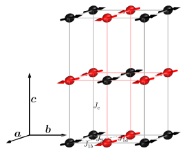
To deal with the striped AFM configuration of LaFeAsO, we consider the Fe lattice of the original orthorhombic LaFeAsO structure and divide it into two sublattices in each of which the Fe spins align parallel but antiparallel between the two sublattices (figure 1). Hence we consider an anisotropic Heisenberg Hamiltonian

$$\hat{H}=\sum_{\langle\mathbf{i,j}\rangle}J_{\langle\mathbf{i,j}\rangle}\mathbf{\hat{S}_{i}}\cdot\mathbf{\hat{S}_{j}}+J_{2}\sum_{\langle\!\langle\mathbf{i,j}\rangle\!\rangle}\mathbf{\hat{S}_{i}}\cdot\mathbf{\hat{S}_{j}}~{},$$ (1)

in which $\mathbf{\hat{S}}_{\mathbf{i}}$ denotes the quantum spin operator at the lattice position $\mathbf{i}$, $\langle\mathbf{i,j}\rangle$ means nearest-neighbour (NN) spin pairs, and $\langle\!\langle\mathbf{i,j}\rangle\!\rangle$ means next-nearest-neighbour (NNN) spin pairs in $a$-$b$ plane (we only consider NNN pairs in $a$-$b$ plane because the inter-layer interactions are very weak). NN interaction $J_{\langle\mathbf{i,j}\rangle}$ can be three values: $J_{1a}$ which is the spin interaction between parallel NN spins in $a$-$b$ plane, $J_{1b}$ between antiparallel NN spins in $a$-$b$ plane and $J_{c}$ between inter-layer NN spins. $J_{2}$ is interaction between NNN spins in $a$-$b$ plane. Four different $J$’s make $\hat{H}$ anisotropic. To differentiate spin operators in SL1 and SL2, we use $\mathbf{\hat{S}}_{1\mathbf{i}}$ and $\mathbf{\hat{S}}_{2\mathbf{j}}$ to represent them respectively. For spins in SL2, we make transformations: $\hat{S^{\prime}}\vphantom{\hat{S}}^{\phantom{\prime}}_{\!\!2\mathbf{j}}{\!\!\!{}^{z}}=-\hat{S}_{2\mathbf{j}}^{z}$, $\hat{S^{\prime}}\vphantom{\hat{S}}^{\phantom{\prime}}_{\!\!2\mathbf{j}}{\!\!\!{}^{+}}=\hat{S}_{2\mathbf{j}}^{-}$, $\hat{S^{\prime}}\vphantom{\hat{S}}^{\phantom{\prime}}_{\!\!2\mathbf{j}}{\!\!\!{}^{-}}=\hat{S}_{2\mathbf{j}}^{+}$ and then have

$$\eqalign{\mathbf{\hat{S}}_{1\mathbf{i}}\cdot\mathbf{\hat{S}}_{2\mathbf{j}}&={\displaystyle\frac{1}{2}}(\hat{S}_{1\mathbf{i}}^{+}\hat{S}_{2\mathbf{j}}^{-}+\hat{S}_{1\mathbf{i}}^{-}\hat{S}_{2\mathbf{j}}^{+})+\hat{S}_{1\mathbf{i}}^{z}\hat{S}_{2\mathbf{j}}^{z}\\ &={\displaystyle\frac{1}{2}}(\hat{S}_{1\mathbf{i}}^{+}\hat{S^{\prime}}\vphantom{\hat{S}}^{\phantom{\prime}}_{\!\!2\mathbf{j}}{\!\!\!{}^{+}}+\hat{S}_{1\mathbf{i}}^{-}\hat{S^{\prime}}\vphantom{\hat{S}}^{\phantom{\prime}}_{\!\!2\mathbf{j}}{\!\!\!{}^{-}})-\hat{S}_{1\mathbf{i}}^{z}\hat{S^{\prime}}\vphantom{\hat{S}}^{\phantom{\prime}}_{\!\!2\mathbf{j}}{\!\!\!{}^{z}}~{}.}$$ (2)

Inserting (2) into (1) we can get the Hamiltonian expressed by $\mathbf{S}_{1\mathbf{i}}$ and $\mathbf{S}^{\prime}_{2\mathbf{j}}$ (simple but too long to give out here).

Figure 1: The magnetic cell with volume $a\times 2b\times 2c$ of the orthorhombic Fe spin lattice. The Fe lattice consists of two spin sublattices: SL1 (black) and SL2 (red or gray). ${\bi{a}}$ and ${\bi{b}}$ are the two base vectors in the FeAs layer, and ${\bi{c}}$ is perpendicular to both of ${\bi{a}}$ and ${\bi{b}}$.

Accordingly, we use Green’s function method[27, 28] to solve the model (1). In this scheme one uses a double-time Green’s function $\langle\!\langle\hat{A}(t);\hat{B}(t^{\prime})\rangle\!\rangle$ ($\hat{A}$ and $\hat{B}$ represent two arbitrary quantum operators) which satisfies the following equation of motion:

$$\rmi\hbar\frac{\mathrm{d}}{\mathrm{d}t}\langle\!\langle\hat{A} (t);\hat{B}(t^{\prime})\rangle\!\rangle=$$ (3)

$$\delta(t-t^{\prime})\langle[\hat{A}(t),\hat{B}(t)]\rangle+\langle\!\langle[\hat{A}(t),\hat{H}];\hat{B}(t^{\prime})\rangle\!\rangle.$$

This approach proves successful for various Heisenberg spin models [27, 28, 29, 30, 31, 32]. In [30], there is a detailed but somewhat long derivation about the Green’s function method for Heisenberg spin model. Accordingly, we sum up the derivation in [30] and get the point that the process of using Green’s functions to solve the average spin of Heisenberg model can be simplified into three steps: a) construct Green’s functions $\langle\!\langle\hat{S}^{+}_{\mathbf{i}};\hat{S}^{-}_{\mathbf{j}}\rangle\!\rangle$ and their equations of motion via (3) and then use Tyablikov cutoff approximation (4) to decouple the equations of motion[28];

$$\langle\!\langle\hat{S}^{z}_{\mathbf{i}}\hat{S}^{+}_{\mathbf{j}};\hat{B}\rangle\!\rangle\longrightarrow^{\mathbf{i}\neq\mathbf{j}}~{}\langle\hat{S}^{z}\rangle\langle\!\langle\hat{S}^{+}_{\mathbf{j}};\hat{B}\rangle\!\rangle$$ (4)

b) use spectrum theorem to express the correlation function $\langle\hat{S}^{-}\hat{S}^{+}\rangle$ in term of the average spin $z$-component $\langle\hat{S}^{z}\rangle$ and then get the $\Phi(\langle\hat{S}^{z}\rangle)$ function

$$\Phi(\langle\hat{S}^{z}\rangle)=\frac{1}{2}\langle\hat{S}^{-}\hat{S}^{+}\rangle/\langle\hat{S}^{z}\rangle~{};$$ (5)

c) use the Callen Expression (6)[30] to evaluate $\langle\hat{S}^{z}\rangle$ self-consistently

$$\langle\hat{S}^{z}\rangle={\displaystyle\frac{(S-\Phi)(1+\Phi)^{2S+1}+(S+1+\Phi)\Phi^{2S+1}}{(1+\Phi)^{2S+1}-\Phi^{2S+1}}}~{}.$$ (6)

According to the three steps given above, for our spin system we construct double-time spin Green’s functions between spin operators at two positions $\mathbf{i}$ and $\mathbf{j}$ in SL1

$$\widetilde{G}_{\mathbf{ij}}^{\scriptscriptstyle{(11)}}(t,t^{\prime})=\langle\!\langle\hat{S}_{1\mathbf{i}}^{+}(t);\hat{S}_{1\mathbf{j}}^{-}(t^{\prime})\rangle\!\rangle$$ (7)

and Green’s functions between spin operators at two positions $\mathbf{i}^{\prime}$ in SL2 and $\mathbf{j}^{\prime}$ in SL1

$$\widetilde{G}_{\mathbf{i}^{\prime}\mathbf{j}^{\prime}}^{\scriptscriptstyle{(21)}}(t,t^{\prime})=\langle\!\langle\hat{S^{\prime}}\vphantom{\hat{S}}^{\phantom{\prime}}_{\!\!2\mathbf{i\mbox{\unboldmath$\scriptscriptstyle{{}^{\prime}}$}}}{\!\!\!{}^{\!\!-}}(t);\hat{S}_{1\mathbf{j}^{\prime}}^{-}(t^{\prime})\rangle\!\rangle~{}.$$ (8)

Equation (7) can be expressed as Fourier expansion

$$\widetilde{G}^{\scriptscriptstyle{(11)}}_{\mathbf{ij}}(t,t^{\prime})=\frac{1}{2\pi\hbar}\int G^{\scriptscriptstyle{(11)}}_{\mathbf{ij}}(\omega)\rme^{-\rmi\omega(t-t^{\prime})/\hbar}\mathrm{d}\omega,$$ (9)

because the Hamiltonian (1) is time independent, and (8) is similar. Assuming that each spin has the same average $\langle\hat{S}_{1}^{z}\rangle$ for SL1 and $\langle\hat{S^{\prime}_{2}}{\!{}^{z}}\rangle$ for SL2 and because of the AFM symmetry plus the transformation (2), we have $\langle\hat{S}_{1}^{z}\rangle=\langle\hat{S^{\prime}_{2}}{\!{}^{z}}\rangle=\langle\hat{S}^{z}\rangle$. Then using the Fourier transformation as shown in (9), making Tyablikov cutoff approximation to decouple the equations of motion and another Fourier transformation from lattice sites real space to $\mathbf{k}$ space, we can have

$$1+g_{\mathbf{k}}^{\scriptscriptstyle{(11)}}\bigg{[}J_{1b}\rho_{{}_{1}}(\mathbf{k})-\frac{\omega}{2\langle\hat{S}^{z}\rangle}\bigg{]}+J_{1b}g_{\mathbf{k}}^{\scriptscriptstyle{(21)}}\rho_{{}_{2}}(\mathbf{k})=0~{}$$ (10)

and

$$g_{\mathbf{k}}^{\scriptscriptstyle{(11)}}J_{1b}\rho_{{}_{2}}(\mathbf{k})+g_{\mathbf{k}}^{\scriptscriptstyle{(21)}}\bigg{[}J_{1b}\rho_{{}_{1}}(\mathbf{k})+\frac{\omega}{2\langle\hat{S}^{z}\rangle}\bigg{]}=0~{},$$ (11)

in which

$$\eqalign{g_{\mathbf{k}}^{\scriptscriptstyle{(11)}}&=\sum_{\mathbf{r}}G_{\mathbf{i},\mathbf{i}+\mathbf{r}}^{\scriptscriptstyle{(11)}}(\omega)\mathrm{e}^{-\rmi\mathbf{k}\cdot\mathbf{r}}\\ g_{\mathbf{k}}^{\scriptscriptstyle{(21)}}&=\sum_{\mathbf{r}}G_{\mathbf{i},\mathbf{i}+\mathbf{r}}^{\scriptscriptstyle{(21)}}(\omega)\mathrm{e}^{-\rmi\mathbf{k}\cdot\mathbf{r}}~{},}$$ (12)

$$\eqalign{\rho_{{}_{1}}(\mathbf{k})&=-p(1-\cos\mathbf{k}\!\cdot\!{\bi{a}})+1+2q+r\\ \rho_{{}_{2}}(\mathbf{k})&=(1+2q\cos\mathbf{k}\!\cdot\!{\bi{a}})\cos\mathbf{k}\!\cdot\!{\bi{b}}+r\cos\mathbf{k}\!\cdot\!{\bi{c}}~{},}$$ (13)

and

$$p\equiv\frac{J_{1a}}{J_{1b}}~{},~{}~{}q\equiv\frac{J_{2}}{J_{1b}}~{},~{}~{}r\equiv\frac{J_{c}}{J_{1b}}~{}.$$ (14)

We should point out that: a) the wave vector $\mathbf{k}$ we used here is based on the whole lattice sites (SL1+SL2), so $\mathbf{r}$ in summations of (12) runs over all sites in the whole lattice; b) for homogeneous system $G_{\mathbf{i},\mathbf{i}+\mathbf{r}}^{\scriptscriptstyle{(11)}}$ is only a function of relative position $\mathbf{r}$ and independent of $\mathbf{i}$ (as a result $G_{\mathbf{ii}}^{\scriptscriptstyle{(11)}}=G^{\scriptscriptstyle{(11)}}$ which is used below); $G_{\mathbf{i},\mathbf{i}+\mathbf{r}}^{\scriptscriptstyle{(21)}}$ is analogous.

From (10) and (11) we derive

$$g_{\mathbf{k}}^{\scriptscriptstyle{(11)}}=\frac{\langle\hat{S}^{z}\rangle}{\sqrt{\rho_{{}_{1}}^{2}\!-\!\rho_{{}_{2}}^{2}}}\bigg{[}\frac{\rho_{{}_{1}}\!+\!\sqrt{\rho_{{}_{1}}^{2}\!-\!\rho_{{}_{2}}^{2}}}{\omega-E(\mathbf{k})}-\frac{\rho_{{}_{1}}\!-\!\sqrt{\rho_{{}_{1}}^{2}\!-\!\rho_{{}_{2}}^{2}}}{\omega+E(\mathbf{k})}\bigg{]},$$ (15)

where $E({\mathbf{k}})$ is the spin excitation spectrum defined by

$$E(\mathbf{k})=2J_{1b}\langle\hat{S}^{z}\rangle\sqrt{\rho_{{}_{1}}^{2}(\mathbf{k})-\rho_{{}_{2}}^{2}(\mathbf{k})}~{}.$$ (16)

And from $g_{\mathbf{k}}^{\scriptscriptstyle{(11)}}$ we get $G_{\mathbf{ij}}^{\scriptscriptstyle{(11)}}$

$$G_{\mathbf{ij}}^{\scriptscriptstyle{(11)}}(\omega)=\frac{1}{N}\sum_{\mathbf{k}\in{\rm BZ}}g_{\mathbf{k}}^{\scriptscriptstyle{(11)}}\mathrm{e}^{\rmi\mathbf{k}\cdot(\mathbf{i}-\mathbf{j})}~{},$$ (17)

in which $N$ is the total number of spins in SL1 and SL2, and BZ denotes the first Brillouin zone (there are $N$ $\mathbf{k}$-points in BZ). Using spectrum theorem and letting $\mathbf{j}=\mathbf{i}$ we get the correlation function $\langle\hat{S}_{1}^{-}\hat{S}_{1}^{+}\rangle$ as follow

$$\eqalign{\langle\hat{S}_{1}^{-}\hat{S}_{1}^{+}\rangle&=-\frac{1}{\pi}\int_{-\infty}^{\infty}{\displaystyle\frac{\mathrm{Im}[G^{\scriptscriptstyle{(11)}}(\omega+i0^{+})]}{\mathrm{e}^{\beta\omega}-1}}\mathrm{d}\omega\\ &=\frac{\langle\hat{S}_{1}^{z}\rangle}{N}\sum_{\mathbf{k}\in{\rm BZ}}\bigg{[}\frac{\rho_{{}_{1}}}{\sqrt{\rho_{{}_{1}}^{2}-\rho_{{}_{2}}^{2}}}\coth\frac{\beta E(\mathbf{k})}{2}-1\bigg{]}~{},}$$ (18)

where $\beta=1/(k_{{}_{\rm B}}T)$, $T$ is temperature, and $k_{{}_{\rm B}}$ is the Boltzmann constant. Then using (5) we get the $\Phi$ function:

$$\Phi(\langle\hat{S}^{z}\rangle)=\frac{1}{2N}\sum_{\mathbf{k}\in{\rm BZ}}\bigg{[}\frac{\rho_{{}_{1}}}{\sqrt{\rho_{{}_{1}}^{2}-\rho_{{}_{2}}^{2}}}\coth\frac{\beta E(\mathbf{k})}{2}-1\bigg{]}~{}.$$ (19)

Now, the average spin $z$-component $\langle\hat{S}^{z}\rangle$ can be obtained easily by self-consistently solving (19) and (6). A special case is that when the temperature $T=0$, $\coth\frac{\beta E(\mathbf{k})}{2}\rightarrow 1$ and we have

$$\Phi_{0}\equiv\Phi|_{T=0}=\frac{1}{2N}\sum_{\mathbf{k}\in{\rm BZ}}\bigg{[}\frac{\rho_{{}_{1}}}{\sqrt{\rho_{{}_{1}}^{2}-\rho_{{}_{2}}^{2}}}-1\bigg{]}~{}.$$ (20)

At this time, $\Phi_{0}$ is no longer dependent on $\langle\hat{S}^{z}\rangle$ and the zero-temperature average spin $z$-component ${\langle\hat{S}^{z}\rangle}_{\!\scriptscriptstyle{0}}$ can be obtained directly by insert (20) into (6).

While temperature approaches to $T_{\rm N}$, $\langle\hat{S}^{z}\rangle$ approaches to zero and further $E(\mathbf{k})\rightarrow 0$ and $\Phi\rightarrow\infty$. Expanding (19) and (6), we derive

$$\langle\hat{S}^{z}\rangle\propto\sqrt{1-\frac{T}{T_{\rm N}}}~{},$$ (21)

where $T_{\rm N}$ is defined by

$$T_{\rm N}=\frac{2J_{1b}S(S+1)}{3\Gamma k_{{}_{\rm B}}}$$ (22)

and $\Gamma=\frac{1}{N}\sum_{\mathbf{k}}[\rho_{{}_{1}}/(\rho_{{}_{1}}^{2}-\rho_{{}_{2}}^{2})]$.

3 Numerical Results and discussions

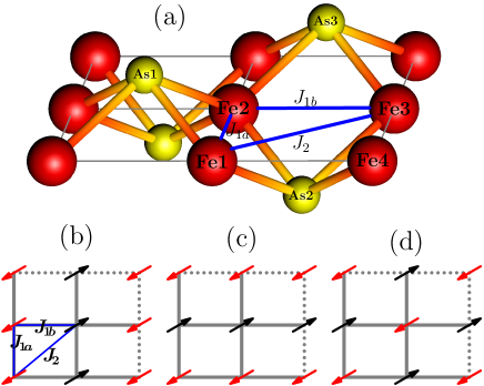
Figure 2: (a) Structure of FeAs layer and scheme for the exchange interactions mediated by Fe-As-Fe paths: Fe1-As1-Fe2 and Fe1-As2-Fe2 for $J_{1a}$, Fe2-As2-Fe3 and Fe2-As3-Fe3 for $J_{1b}$, and Fe1-As2-Fe3 for $J_{2}$. Different AFM configurations are shown: (b) stripe-AFM along ${\bi{a}}$ direction, (c) stripe-AFM along ${\bi{b}}$ direction, and (d) checkerboard AFM. Energies of the three AFM configurations are given in (23).

About the coupling interactions $J_{1a}$, $J_{1b}$, $J_{2}$ and $J_{c}$ in FeAs-based pnictides, there is no consensus on their magnitudes and many authors only consider two or three of them[4, 5, 33, 23, 19, 16, 34]. Yildirim’s first-principles results show that $J_{1}\sim J_{2}$[5]. However, we prefer the opinion that $J_{1a}$, $J_{1b}$ and $J_{2}$ originate from AFM superexchange through As atoms[35, 36, 37]. From the viewpoint of the structure of FeAs layers, both $J_{1a}$ and $J_{1b}$ are mediated by two Fe-As-Fe paths (figure 2(a)) and there should be $J_{1a}\neq J_{1b}$ but $J_{1a}\sim J_{1b}$ due to the small structure change from tetragonal to orthorhombic symmetry. $J_{2}$ is mediated by only one Fe-As-Fe path (figure 2(a)) and there should be $2J_{2}\sim J_{1a}$. From the viewpoint of classical favorable energy to form stripe-like AFM patterns along ${\bi{a}}$ direction as shown in figure 2(b) (see figure 2(b)-(d) and (23)),

$$\left\{\eqalign{E_{{\rm(b)}}&=\phantom{+}4J_{1a}S^{2}-4J_{1b}S^{2}-8J_{2}S^{2}\\ E_{{\rm(c)}}&=-4J_{1a}S^{2}+4J_{1b}S^{2}-8J_{2}S^{2}\\ E_{{\rm(d)}}&=-4J_{1a}S^{2}-4J_{1b}S^{2}+8J_{2}S^{2}~{}\\ E_{{\rm(b)}}&<E_{{\rm(c)}}~{}\Longrightarrow~{}J_{1a}<J_{1b}\\ E_{{\rm(b)}}&<E_{{\rm(d)}}~{}\Longrightarrow~{}2J_{2}>J_{1a}}\right.$$ (23)

there should be $J_{1a}<J_{1b}$ and $2J_{2}>J_{1a}$, which in fact are just the conditions that fulfill $\rho_{{}_{1}}^{2}-\rho_{{}_{2}}^{2}\geqslant 0$ to make $E(\mathbf{k})$ in (16) meaningful. As for $J_{c}$, it’s a very weak long-range AFM interaction with a nowadays unclear origin other than superexchange. Therefore, in terms of $p,~{}q,~{}r$ in (14) we confine the coupling interactions as follow:

$$\left\{\eqalign{&1\geqslant p\geqslant 1-\delta_{p}\\ &p/2<q\leqslant p/2+\delta_{q}~{},\\ &0<r\leqslant\delta_{r}}\right.$$ (24)

where $\delta_{p}$, $\delta_{q}$, and $\delta_{r}$ are the confine parameters for $p$, $q$, and $r$ respectively and they fulfill $0<\delta_{p},\delta_{q},\delta_{r}\ll 1$. Lhs of (24) represents the necessary conditions to form striped AFM ordering along ${\bi{a}}$ direction, and rhs the conditions to limit $p$, $q$ and $r$ within small regions.

Figure 3: The reduced AFM transition temperatures ($T_{\rm N}/[J_{1b}S(S+1)]$) as functions of $q$ for $r=0.001$ and $p=0.90,0.92,\cdots,1.0$ (from top to bottom). The inset shows an $r$ dependence of $T_{\rm N}$ for $p=0.98$ and $q=0.5$.

From figure 3 we can see that $T_{\rm N}$ increases as $q$ and $r$ increase but decreases as $p$ increases. It’s easy to understand. NNN spins and inter-layer NN spins all align antiparallel, so bigger AFM coupling interactions will lower the system’s energy, stabilize the AFM configuration and hence enhance $T_{\rm N}$; on the contrary, spins along ${\bi{a}}$ direction align parallel but have AFM interactions, therefore bigger $p$ will increase the system’s energy, destabilize the AFM configuration and hence decrease $T_{\rm N}$. It’s notable that while $q\rightarrow p/2$ or $r\rightarrow 0$, then $T_{\rm N}\rightarrow 0$, that is to say, both the existence of an AFM inter-layer interaction $J_{c}$ and the condition $2J_{2}>J_{1a}$ are essential to form striped AFM ordering. In fact, when $r=0$ this system becomes two-dimensional, and the result of $T_{\rm N}=0$ in two dimensions is analogous to the Mermin-Wagner theorem for isotropic interactions[38]. We also see that the critical condition $p=1$ doesn’t lead to $T_{\rm N}\rightarrow 0$, which manifests $J_{1a}=J_{1b}$ isn’t a fatal factor to kill $T_{\rm N}$ but only a critical value to separate the two cases shown in figure 2(b) and 2(c).

Figure 4: The zero-temperature average spins ${\langle\hat{S}^{z}\rangle}_{\!\scriptscriptstyle{0}}$ as functions of $q$ for $r=0.001$ and different $p$ values: $0.90,0.92,\cdots,1.0$. The lower limits of ${\langle\hat{S}^{z}\rangle}_{\!\scriptscriptstyle{0}}$ are shown by the dotted line. The inset shows ${\langle\hat{S}^{z}\rangle}_{\!\scriptscriptstyle{0}}\sim r$ curves for $(p,q)=(0.98,0.50)$ (solid) and $(0.98,0.49)$ (dotted) respectively.

Magnetic moment per Fe of LaFeAsO at low temperature is reported as 0.36$\mu_{{\rm B}}$[2] or 0.25$\mu_{{\rm B}}$[3] experimentally, both of which are very small compared with the first-principles values $2.2\sim 2.4\mu_{{\rm B}}$/Fe[39, 40]. Accordingly, we choose $S=1$ in our model (assuming the Landé $g$-factor equals 2). Figure 4 shows the zero-temperature average spin ${\langle\hat{S}^{z}\rangle}_{\!\scriptscriptstyle{0}}$. Similar to $T_{\rm N}$, ${\langle\hat{S}^{z}\rangle}_{\!\scriptscriptstyle{0}}$ is also an increasing function of both $q$ and $r$ but a decreasing function of $p$. However, ${\langle\hat{S}^{z}\rangle}_{\!\scriptscriptstyle{0}}\rightarrow 0$ only when both $r\rightarrow 0$ and $q\rightarrow p/2$. When only $r\rightarrow 0$ or $q\rightarrow p/2$ is met, ${\langle\hat{S}^{z}\rangle}_{\!\scriptscriptstyle{0}}$ approaches to a minimum but not zero, while at the same time $T_{\rm N}\rightarrow 0$.

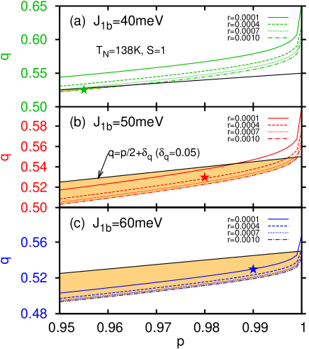
Figure 5: The parameter regions (orange or gray) satisfying (24) with $T_{\rm N}=138$K for $J_{1b}=40$meV (a), $J_{1b}=50$meV (b), and $J_{1b}=60$meV (c), where we use $\delta_{p}=0.05,\delta_{q}=0.05$, and $\delta_{r}=0.001$. The star shows the value $(p,q,r)$=(0.955, 0.526, 0.0009) in (a), (0.98, 0.53, 0.0003) in (b), or (0.99, 0.53, 0.0001) in (c).

There are four $J$’s in our model. What are their values? Then let us have a look at what can they be under condition $T_{\rm N}=138$K. Figure 5 shows the regions available for $p$, $q$ and $r$ under conditions (24) with $\delta_{p}=0.05,\delta_{q}=0.05$ and $\delta_{r}=0.001$ in orange (gray) colour for $J_{1b}=40$meV, 50meV, and 60meV respectively. The smaller $J_{1b}$, the smaller the parameter region available. Hence, for given $\delta_{p}$, $\delta_{q}$ and $\delta_{r}$, there is a lower limit for $J_{1b}$ to fulfill a given $T_{\rm N}$. This lower limit, written as $J_{1b}^{{\rm min}}$, is given in table 1, which shows that the smaller each of $\delta_{p}$, $\delta_{q}$ and $\delta_{r}$ is, the bigger $J_{1b}^{{\rm min}}$ is. However, although no upper limit for $J_{1b}$ is given out, $J_{1b}$ can not be infinitely great. In fact, first-principles results show that $J_{1b}\sim 50$meV[4, 33].

Here we didn’t use the experimental data for low-temperature magnetic moment per Fe atom, which amounts to ${\langle\hat{S}^{z}\rangle}_{\!\scriptscriptstyle{0}}=0.13\sim 0.18$, to determine the $J$’s, because it’s too small. If ${\langle\hat{S}^{z}\rangle}_{\!\scriptscriptstyle{0}}=0.18$ is met, there have to be $\delta_{r}<10^{-6}$ even if $q=p/2$ is taken to minimize ${\langle\hat{S}^{z}\rangle}_{\!\scriptscriptstyle{0}}$ (see inset of figure 4). Such tiny $r$ definitely cannot fall within the orange (gray) area in figure 5 with a reasonable $J_{1b}$ to fulfill $T_{\rm N}=138$K. That is to say, although the many-body AFM fluctuations substantially reduce the low-temperature magnetic moment per Fe, yet they cannot be in full charge of the very small low-temperature magnetic moment which indeed is also ascribed to spin orbit and $p$-$d$ hybridization etc[6].

Table 1: $J_{1b}^{{\rm min}}$ for given $\delta_{p}$, $\delta_{q}$ and $\delta_{r}$.

• $\hskip 14.22636pt\delta_{q}\hskip 14.22636pt$	$\delta_{r}$	$\delta_{p}$	$J_{1b}^{{\rm min}}$/meV
  0.01	0.0001	0.01	104.4
  		0.1	89.8
  	0.001	0.01	87.1
  		0.1	72.6
  0.05	0.0001	0.01	50.9
  		0.1	44.6
  	0.001	0.01	43.6
  		0.1	37.2

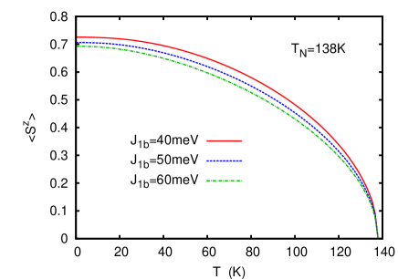
We choose three sets of $J$’s from the regions available in figure 5 for estimation (the three stars): $(p,q,r)$=(0.955, 0.526, 0.0009), (0.98, 0.53, 0.0003), and (0.99, 0.53, 0.0001) for $J_{1b}$=40meV, 50meV, and 60meV respectively. In terms of $J_{1b}$, $J_{1a}$, $J_{2}$ and $J_{c}$, we can refer to them as $J_{1b}=50\pm 10$meV, $J_{1a}=49\pm 10$meV, $J_{2}=26\pm 5$meV, and $J_{c}=0.020\pm 0.015$meV. The average spin $\langle\hat{S}^{z}\rangle$ vs temperature $T$ curves with the three sets of parameters given above are shown in figure 6.

Figure 6: The average spins $\langle\hat{S}^{z}\rangle$ as functions of the temperature $T$ for $J_{1b}$=40meV, 50meV, and 60meV. The corresponding $(p,q,r)$ parameters are (0.955, 0.526, 0.0009), (0.98, 0.53, 0.0003), and (0.99, 0.53, 0.0001), respectively.

We take LaFeAsO for example here, however our calculations are not restricted to LaFeAsO, because nearly all $Ln$FeAsO has similar even the same transition temperatures (see table 2).

Table 2: AFM and structure transition temperatures $T_{\rm N}$ and $T_{\rm S}$ of $Ln$FeAsO.

• $Ln$	La	Ce	Pr	Nd	Sm
  $T_{\rm N}$(K)	138	140	127	141	140
  $T_{\rm S}$(K)	156	155	153	-	-
  Ref	[3]	[8]	[10]	[11]	[41]

It seems that $T_{\rm N}$ doesn’t vary much with different $Ln$. This is different from $A$Fe₂As₂, whose $T_{\rm N}$ varies with $A$: $T_{\rm N}$=172.5K[18] for $A$=Ca; $T_{\rm N}$=198K[20], 205K[42] or 220K[43] for $A$=Sr and $T_{\rm N}$=140K[22] or 135K[44] for $A$=Ba. Although there are some differences of structure between $Ln$FeAsO and $A$Fe₂As₂, we believe that our model works well for both of them, because they both have layered structures with stripe-like AFM order formed by Fe atoms. Indeed, this can also be extended to Fe(SeTe)[45, 46], which also have nearly the same properties and can be superconducting under certain conditions.

4 Conclusion

In summary, we use a Green’s function method to study the striped AFM order formed by Fe atoms in $Ln$FeAsO which is the representative of the parent compounds of recently discovered Fe-based superconductors. We take LaFeAsO for example to analyze the AFM transition temperature $T_{\rm N}$ and zero-temperature average spin ${\langle\hat{S}^{z}\rangle}_{\!\scriptscriptstyle{0}}$, and show that both $T_{\rm N}$ and ${\langle\hat{S}^{z}\rangle}_{\!\scriptscriptstyle{0}}$ are increasing functions of $J_{1b}$, $J_{2}$ and $J_{c}$ but decreasing functions of $J_{1a}$. By using $T_{\rm N}=138$K, we make a reasonable estimation of the coupling interactions, $J_{1b}=50\pm 10$meV, $J_{1a}=49\pm 10$meV, $J_{2}=26\pm 5$meV, and $J_{c}=0.020\pm 0.015$meV. Average spin $\langle\hat{S}^{z}\rangle$ is determined in the same way from zero temperature to $T_{\rm N}$ and $T_{\rm N}$ is expressed analytically. Our results also show that a non-zero AFM inter-layer coupling $J_{c}$ is essential to the existence of a non-zero $T_{\rm N}$ and that the AFM fluctuations substantially reduce the low-temperature magnetic moment towards the small experimental value. Although our results cannot determine the relations between structure and AFM transitions, we believe that the AFM transition is likely caused by the structure transition because most of experimental results show $T_{\rm N}\leqslant T_{\rm S}$ for FeAs-based pnictides. Our Green’s function approach of the striped AFM properties can be used to other FeAs-based parent compounds.

References

• [1] Kamihara Y, Watanabe T, Hirano M and Hosono H 2008 J. Am. Chem. Soc. 130 3296
• [2] de la Cruz C et al 2008 Nature 453 899
• [3] Klauss H H et al 2008 Phys. Rev. Lett. 101 077005
• [4] Yin Z P, Lebègue S, Han M J, Neal B P, Savrasov S Y and Pickett W E 2008 Phys. Rev. Lett. 101 047001
• [5] Yildirim T 2008 Phys. Rev. Lett. 101 057010
• [6] Wu J, Phillips P and Castro Neto A H 2008 Phys. Rev. Lett. 101 126401
• [7] Fang C, Yao H, Tsai W F, Hu J P and Kivelson S A 2008 Phys. Rev. B 77 224509
• [8] Zhao J et al 2008 Nat. Mater. 7 953
• [9] Chen G F, Li Z, Wu D, Li G, Hu W Z, Dong J, Zheng P, Luo J L and Wang N L 2008 Phys. Rev. Lett. 100 247002
• [10] Zhao J et al 2008 Phys. Rev. B 78 132504
• [11] Chen Y, Lynn J W, Li J, Li G, Chen G F, Luo J L, Wang N L, Dai P, dela Cruz C and Mook H A 2008 Phys. Rev. B 78 064515
• [12] Jia Y, Cheng P, Fang L, Luo H, Yang H, Ren C, Shan L, Gu C and Wen H H 2008 Appl. Phys. Lett. 93 032503
• [13] Chen X H, Wu T, Wu G, Liu R H, Chen H and Fang D F 2008 Nature 453 761
• [14] Ding L, He C, Dong J K, Wu T, Liu R H, Chen X H and Li S Y 2008 Phys. Rev. B 77 180510(R)
• [15] Drew A J et al 2008 Phys. Rev. Lett. 101 097010
• [16] McQueeney R J et al 2008 Phys. Rev. Lett. 101 227205
• [17] Torikachvili M S, Bud’ko S L, Ni N and Canfield P C 2008 Phys. Rev. Lett. 101 057006
• [18] Goldman A I, Argyriou D N, Ouladdiaf B, Chatterji T, Kreyssig A, Nandi S, Ni N, Bud’ko S L, Canfield P C and McQueeney R J 2008 Phys. Rev. B 78 100506(R)
• [19] Zhao J et al 2008 Phys. Rev. Lett. 101 167203
• [20] Yan J Q et al 2008 Phys. Rev. B 78 024516
• [21] Hu W Z, Dong J, Li G, Li Z, Zheng P, Chen G F, Luo J L and Wang N L 2008 Phys. Rev. Lett. 101 257005
• [22] Rotter M, Tegel M, Johrendt D, Schellenberg I, Hermes W and Pöttgen R 2008 Phys. Rev. B 78 020503(R)
• [23] Ewings R A, Perring T G, Bewley R I, Guidi T, Pitcher M J, Parker D R, Clarke S J and Boothroyd A T 2008 Phys. Rev. B 78 220501(R)
• [24] Qiu Y et al 2008 Phys. Rev. B 78 052508
• [25] Pfuner F, Analytis J G, Chu J H, Fisher I R and Degiorgi L 2008 arXiv:0811.2195v1 [cond-mat]
• [26] Yao D X and Carlson E W 2008 Phys. Rev. B 78 052507
• [27] Bogoliubov N N and Tyablikov S V 1959 Dokl. Akad. Nauk SSSR 126 53
• [28] Tyablikov S V 1959 Ukr. Mat. Zh. 11 287
• [29] Tahir-Kheli R A and ter Haar D 1962 Phys. Rev. 127 88
• [30] Callen H B 1963 Phys. Rev. 130 890
• [31] Liu B G 1990 Phys. Rev. B 41 9563
• [32] Liu B G and Pu F C 2001 J. Mag. Mag. Mater. 231 307
• [33] Ma F, Lu Z Y and Xiang T 2008 Phys. Rev. B 78 224517
• [34] Yaresko A N, Liu G Q, Antonov V N and Andersen O K 2008 arXiv:0810.4469v1 [cond-mat]
• [35] Si Q and Abrahams E 2008 Phys. Rev. Lett. 101 076401
• [36] Jishi R A and Alyahyaei H M 2008 arXiv:0811.2716v1 [cond-mat]
• [37] Belashchenko K D and Antropov V P 2008 Phys. Rev. B 78 212515
• [38] Mermin N D and Wagner H 1966 Phys. Rev. 17 1133
• [39] Ma F and Lu Z Y 2008 Phys. Rev. B 78 033111
• [40] Yildirim T 2009 Phys. Rev. Lett. 102 037003
• [41] Martinelli A et al 2008 Supercond. Sci. Technol. 21 095017
• [42] Kumar M, Nicklas M, Jesche A, Caroca-Canales N, Schmitt M, Hanfland M, Kasinathan D, Schwarz U, Rosner H and Geibel C 2008 Phys. Rev. B 78 184516
• [43] Zhao J, Ratcliff II W, Lynn J W, Chen G F, Luo J L, Wang N L, Hu J and Dai P 2008 Phys. Rev. B 78 140504(R)
• [44] Kitagawa K, Katayama N, Ohgushi K, Yoshida M and Takigawa M 2008 J. Phys. Soc. Jpn. 77 114709
• [45] Mizuguchi Y, Tomioka F, Tsuda S, Yamaguchi T and Takano Y 2008 Appl. Phys. Lett. 93 152505
• [46] Chen G F, Chen Z G, Dong J, Hu W Z, Li G, Zhang X D, Zheng P, Luo J L and Wang N L 2008 arXiv:0811.1489v1 [cond-mat]