J-transform applied to the detection of Gravitational Waves:
preliminary results

Abstract

We propose to apply to the detection of Gravitational Waves a new method developed for the spectral analysis of noisy time-series of damped oscillators. From the Padé Approximations of the time-series Z-transform, a Jacobi Matrix (J-Matrix) is constructed.

We show that the J-Matrix has bound states with eigenvalues strictly inside the unit circle. Each bound state can be identified with one precise damped oscillator. Beside these bound states, there is an essential spectrum sitting on the unit circle which represents the noise.

In this picture, signal and noise are clearly separated and identified in the complex plane. Furthermore, we show that the J-transform enjoys the exceptional feature of lossless undersampling.

We take advantage of the above properties of the J-transform to develop a procedure for the search of Gravitational Wave bursts in interferometric data series such as those of LIGO and VIRGO projects. Successful application of our procedure to simulated data having a poor signal to noise ratio, highlights the power of our method.

I Introduction

Experimental time-series are always affected by the presence of noise. As long as the signal to noise ratio is not too poor, several filters are available to denoise the data within the framework of Fourier analysis and its variants. All such techniques, on the other hand, have drawbacks jpa and fail when the signal to noise ratio approaches $1$. It is exactly this very high noise case researchers have to deal with when analyzing LIGO and VIRGO data. The preliminary evidence we present here shows that our denoising method, based on the analytic properties of the Z-transform (generating function) of the data zeta , and its subsequent J-Matrix we associate to it, promises a significantly improvement of the detection probability even in the case of highly correlated noise.

Spectral analysis has been dominated by the Fourier transform (and its variants), which is the ideal tool when noise is not too important.

The major drawback of the Fourier transform is its linearity which prevents it to distinguish noise from signal because the Fourier Transform treats the noise on the same foot as the signal, and therefore leaves noise intact.

Furthermore it is clear that the discrete Fourier Transform is nothing but the specialization of the Z-transform to specific points of the complex plane which are the roots of unity. This is important to notice because, as we have shown in Ref. jpa , the roots of unity are noise attractors in the complex plane. That is to say, noise is not distributed uniformly in the complex plane and one should take advantage of this fact to build an algorithm that makes use of this knowledge.

This also explains the poor results of data spectral analysis in the presence of heavy noise produced by the FFT.

One of the most important application of the new introduced J-transform concerns damped oscillating signals, such as those found in nuclear magnetic resonance data bel and in burst gravitational waves bur ; ring .

The present paper is thus organized:

We first show how to construct the successive J-Matrix approximations built on the time-series data.

We then summarize the principal properties of said approximations and outline how such properties can be used to overcome current detection limitations.

Finally, we give an example where we simulate a search for Gravitational Waves Bursts: the aim is to detect a weak short signal embedded in a single sequence of highly correlated noise (very long, compared to the signal length) and to determine the time at which it happens. Our provisional procedure succeeds to detect the signal in a simulated time sequence having a rather poor signal to noise ratio.

II The tridiagonal Jacobi Matrix.

Given a time-series $s_{0},s_{1},s_{2},.....s_{2n},.......$, it is a standard practice zeta to associate to it its Z-transform defined as:

$$Z(z)=\sum_{m\geq 0}s_{m}z^{-m}$$ (1)

It has been shown jpa that the poles of the $\left[\frac{n-1}{n}\right](z)$ Padé Approximant to $Z-transform$ are the eigenvalues of the tridiagonal $n\times n$ Jacobi Matrix

$$J_{n}=\begin{bmatrix}A_{0}&1&0&...&0&0\\ R_{1}&A_{1}&1&0&0&0\\ 0&R_{2}&A_{2}&1&...&0\\ ...&&&&1&0\\ 0&...&0&R_{n-1}&A_{n-1}&1\\ 0&0&...&0&R_{n}&A_{n}\end{bmatrix}$$ (2)

where

$$A_{k}=-(a_{2k}+a_{2k+1})\qquad R_{k}=a_{2k-1}a_{2k}\qquad k\geq 1\qquad a_{0}=0$$ (3)

The $a_{k}$ being the coefficients of the Stieltjes continued fraction expansion of the $Z-transform$.

The zeros of the Z- transform Padé Approximant can be calculated in a similar way, diagonalizing the $(n-1)\times(n-1)$ Jacobi Matrix for the numerator of the Padé Approximant, which is simply the denominator Jacobi Matrix with the first column and first row removed.

The procedure for computing both zeros and poles of the Z-transform therefore consists in the diagonalization of an already tridiagonal matrix; this makes it computationally extremely efficient (the Hessenberg matrix, often used to find the roots of a polynomial is only sparse and therefore less efficient), and allows us to easily calculate hundreds of poles and zeros.

II.1 The spectrum of the Jacobi Matrix.

To any bounded noisy time series can be associated a tridiagonal Hilbert space operator, its $J-Operator$, extension when $n\rightarrow\infty$ of the previously defined $J_{n}$. With probability one (that is: except for a set of input data series of measure zero), the spectrum of this operator is made of two parts ( see Ref. jpa and references therein):

1) A discrete spectrum, made of a finite number of eigenvalues inside the unit circle: each eigenvalue represents a component of the signal made of a finite number of damped oscillators. The corresponding eigenfunctions have finite norm.

From the value $z_{p}$ of the $p^{th}$ eigenvalue, the characteristics of the damped oscillators of the signal can be immediately derived: the frequencies

$$f_{p}=\frac{2n}{T}\frac{\arg z_{p}}{2\pi}$$ (4)

and the damping factors

$$\alpha_{p}=\frac{2n}{T}\log{|z_{p}|}$$ (5)

where $2n$ is the number of data, and $T$ the recording time. ($\frac{2n}{T}$ is the sampling rate)

2) An essential spectrum with support the unit circle. This spectrum is associated with the noise (uncorrelated part of the signal). The corresponding eigenfunctions have infinite norm.

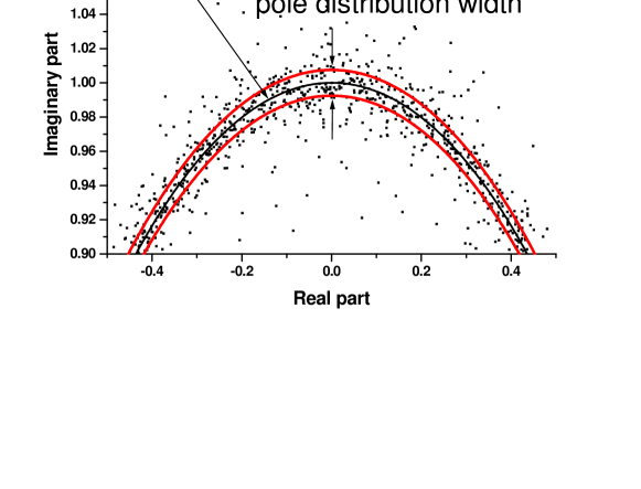
At a finite order, when the infinite $J-Operator$ is truncated, it decomposes into the Froissart poles of the Froissart doublets dou1 ; dou2 ; dou3 ; dou4 (see Figure (1)). The distribution of the poles and zeros of these doublets is universal jpa : independently from the kind of noise, the radial distribution is Lorentzian around the unit circle, with width proportional to$\frac{1}{2n}\ln{2n}$, where $2n$ is the number of data points. The phase distribution is uniform (approaching the $n$ roots of unity when $2n$ goes to infinity).

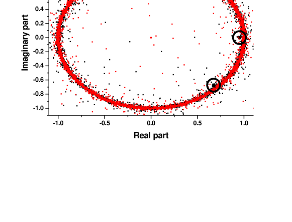
We start by giving a simple straightforward image of the feature of the method. Figure (2) shows poles (black) and zeros (red) of the $Z-transform$ for $40$ different noisy time series of $300$ points each. Each containing the same damped non-oscillating signal, an oscillating one with the same damping factor (again equal for all runs), and a different realization of Gaussian noise. The matched filtering signal to noise ratio $SNR={\frac{\sqrt{\Sigma_{p=1}^{2n}h_{p}^{2}}}{\sigma}}$, where $2n$ is the number of data points, $h_{p}$ are the pure signal points and $\sigma$ is the noise variance, is in this case quite high: $30$ for the non-oscillating signal and $15$ for the oscillating one, so as to have a very clear picture. Most of the poles are around the unit circle and are covered by the corresponding zeros of the Froissart doublets; three clusters of poles (circled in the Figure) inside the unit circle are instead clearly visible: their position is that of the three signal poles.

Here, in order to introduce the method and for the convenience of the reader, we have not yet made use of any of the sophisticated methods developed in the sequel. That is the reason for the use of a high signal to noise ratio.

III Time reversal

If one applies time reversal to a given time-series, one gets a new time-series in which the last term has become the first one and vice-versa.

It is not difficult to check that the denominator of the $Z-transform$ Padé Approximant is covariant under time reversal.

In fact, calling $Q_{n}(z)$ the degree-n polynomial denominator of the Padé Approximant pade

$$Q_{n}=\begin{bmatrix}s_{0}&s_{1}&...&s_{n}\\ s_{1}&s_{2}&...&s_{n+1}\\ ...&...&...&...\\ s_{n-1}&s_{n}&...&s_{2n-1}\\ z^{-n}&z^{-(n-1)}&...&1\end{bmatrix}.$$ (6)

we have the covariant transformation

$$Q_{n}^{T}(z)=z^{n}Q_{n}(\frac{1}{z})$$ (7)

where $Q_{n}^{T}(z)$ is the degree-n polynomial denominator of the Padé Approximant to the time reversal time-series.

Note that this is not true for the zeros of the numerator of the Padé Approximants to the $Z-transform$.

Also, a less formal approach can be provided. The Z-transform of an infinite time series is analytic outside the unit disk under the assumption that it is bounded; this excludes the class of exponentially growing signals.

For a finite time series, exponentially growing signals are instead possible and thus also poles outside the unit disk. From the fact that time inversion transforms a damped signal in an exponentially growing one and vice versa, it is clear that time inversion has to transform all poles $z_{p}$ into their reciprocals $1/z_{p}$.

IV Methods for extracting Spectra from Noisy Data.

In order to make a clear distinction among the poles of the $Z-transform$ of a noisy time series, and identify the eigenvalues corresponding to the discrete spectrum of the$J-Matrix$, we can make use of several properties of the $Z-transform$. Each method we are going to present addressing a different property, a comparison of the results of all methods applicable to any specific time-series is likely to be the optimal choice.

IV.1 Cleaning of Froissart doublets

A first denoising method consists in removing from the complex plane the poles which can be identified as part of Froissart doublets, due to their proximity to zeros of the Z-transform.

This can be done by ordering the poles and zeros in couples in order of increasing distance between the two, and keeping only those whose distance is higher than a given value $\epsilon$ (usually $\epsilon\geq 0.2$).

IV.2 Variational principle

We can on the other hand, making use of the results of section II, search the eigenvalues of Jacobi Matrix associated to the denominator of the Z-transform having modulus strictly smaller than one and for which the norm of the eigenvector have local minima. Such eigenvalues correspond to the frequencies of the signal.

IV.3 Stationariety

It is also possible to compare Padé approximants of different order and look for stable “non-zero paired” poles inside the unit circle: these will be the signal poles, while the non stationary poles will be linked to the noise. This method is particularly useful in dealing with poles in the tails of the noise pole distribution.

IV.4 Undersampling

Another method makes use of the fact that Padé Approximations allow lossless undersampling for the class of damped oscillators jpa .

The above result suggests another technique -which we call “interlaced sampling”- to improve sensitivity when only a single data time-sequence is available. Taking advantage of the undersampling properties of the $Z-transform$, we divide the data in $m$ undersampled sequences, the first one comprising the points $1,m+1,2m+1,3m+1,...$, the second one comprising the points $2,m+2,2m+2,3m+2,...$ and and so on. To first order, the ratio of the width of the pole distribution around the unit circle to the distance of the signal pole from it does not change, but instead of a single signal pole, we do now get a cluster of $m$ poles, which are much easier to detect.

We point out here that we assume to be dealing with data series such that the periods of the signal oscillations to be reconstructed cover several data points. This means that, as long as $m$ is less than the number of data points per period of each of the signal oscillators, the reconstructed signal frequencies will be given by the $m^{th}$ roots of the poles $z_{p}$ having the lowest phases.

IV.5 Time reversal

We have seen that time reversal transforms all poles into their reciprocals. This suggests another way to increase the number of data poles: namely, applying the same procedure using the data in both direct and inverted order.

As the coefficients of the Stieltjes continued fraction expansion of the $Z-transform$ are different in the two cases, the numerically calculated poles will be reciprocal of each others in a nontrivial way.

V An example: Gravitational Waves Bursts

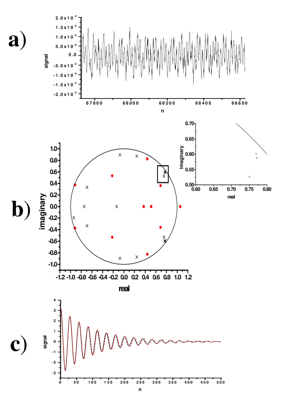
R.Grosso has provided us with simulated data (see Figure (3)) where a “burst” (see Figure (4))is injected on a background “noise” accurately reproducing the correlations found in the data from gravitational waves interferometric detectors grosso ; the matched filtering signal to noise ratio is $SNR\simeq 0.04$. Once the frequencies below $200Hz$, known to contain no signal in the present case, have been filtered out, the “burst” peak amplitude is approximately equal to the background amplitude (see Figure (5)) and the $SNR$ grows to $24$. No assumpion is made on the signal, except that it’s a burst whose duration is of the order of $0.1s$ and whose frequency is higher than $200Hz$.

The basic problem, consisting in detecting a short signal embedded in a single very long sequence and the time at which it happens, is complicated by the fact that the “noise” includes strong fake signals and is therefore highly correlated; this results in a non uniform distribution of the poles and zeros on the unit circle.

Several techniques are currently being used to deal with these two problems in a way that requires direct reading by the operator of only a small set of data, such as change point detection and time-frequency methods. Examples of the former are the BlockNormal method bno , the Excess Power Search method epsm , and the ALF (alternative linear fit) filter alf . Examples of the latter are The WaveBurst algorithm wb and the PSD (power spectral density) method psd .

Up to now, the minimum matched filtering signal to noise ratio allowing signal detection at a significant level using the above methods is around $snr\simeq 15$, assuming Gaussian noise; and $snr\simeq 8$ when the signal is known and it’s possible to use matched filtering sumy . It is, on the other hand, much higher when the above two conditions are not met sumy , as in the present case.

The provisional procedure we describe in the following can be viewed as an extension to the complex plane of the time-frequency methods; it is in no way definitive. Our aim here is to show that the J-transform can be an effective tool in this kind of search:

1) We divide the sequence in 235 blocks of 903 data each.

2) The data in each block gets divided in 3 undersampled sequences of 301 data each, taking the points 1,4,7,10,13,16,19… for the first sequence, the points 2,5,8,11,14,17,20… for the second one and 3,6,9,12,15,18,21… for the third one (“interlaced sampling”).

3) For each undersampled sequence, we clean the Froissart doublets: we calculate the poles and zeros of the [149/150] Padé approximant, we order the poles and zeros in couples in order of increasing distance between the two and keep only those whose distance is higher than 0.2.

4) For each block, we divide the complex plane close to the unit circle in boxes (either square ones or by radius and angle) and take the difference between the number of poles and the number of zeros in each of the boxes.

5) The 3 sequences of each block essentially cover the same signal sequence, they should therefore all 3 give an isolated pole if there is a signal; to be on the safe side we accept 2 out of 3 and therefore keep only the boxes where said number is strictly higher than 1. To make sure not to miss multiple isolated pole occurrences close to the box sides, we repeat the procedure shifting the boxes by 1/2 step.

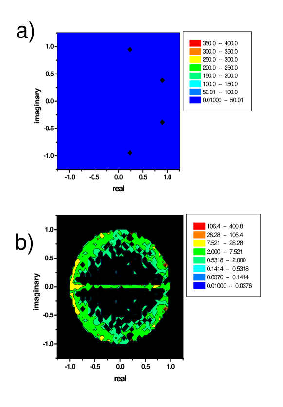
6) Due to the non uniform distribution of the poles and zeros on the unit circle, we observe a number of boxes selected at point 5) which appear in many blocks (see Figure (6)). To get rid of them, we count the number of blocks for which the result for a given box is strictly higher than 1. Boxes for which this number is higher than 3 are discarded.

7) Of the remaining boxes, we keep those appearing only once, or more times but only if this happens in consecutive blocks.

We are left with no consecutive events and only $9$ non-repeated events, each with two poles; closer inspection shows for blocks 63, 76, 215 a third isolated pole close to the two found. (actually, since the data are real, a couple of complex conjugate poles near the other two couples). In all cases it is nonetheless too far away to be reasonably considered related.

8) Considerations of two kinds allow to drop all but block 76. Namely the poles are extremely close to the unit circle, resulting in a signal which is almost constant in amplitude and therefore not a burst, and/or they appear in boxes contiguous to those corresponding to strong noise peaks in Figure (6).

The average position of the selected poles for block 76 allows to reconstruct the clean signal, as shown in Figure (7). As we have not performed a search for the exact position of the signal peak, the signal amplitude was not calculated.

Even using “interlaced sampling” we only have three cases per block. To have some idea of the order of detection probability and false alarm rate, we repeated the search shifting the blocks by $1/4$, $1/2$, and $3/4$ of their length. Considering all $4$ runs, at the end of step 7) only two events appear more than once: the injected signal (3 times out of 4: shift $0$, $1/2$, and $3/4$), and a second event, close to the unit circle, appearing at shifts $1/4$ and $1/2$.

More extensive tests will be needed to properly determine both detection probability and false alarm rate, but the result is encouraging.

VI Conclusion.

In our method, the Z-transform appears as an extension of the discrete Fourier transform to complex values of the frequency: in the complex plane the discrete Fourier transform is the restriction of the Z transform to values of z located at the roots of unity. However, the noise is not uniformly distributed in the complex z-plane and, unfortunately, the roots of unity are noise attractors as shown in Ref. jpa . Therefore, the Fourier transform is not a good choice when a damped signal is embedded in high noise as it is the case in many circumstances. The analytic treatment of the noise we propose, distinguishes, in a drastic way, the signal from the noise by their totally different analytic properties. The fact that the noise presents an analytic characterization that is universal, independent of its statistical properties, has as consequence a much greater independence of the signal identification on the noise level.

The example we have given strongly suggests that the $J-transform$ analysis -especially if coupled with judicious undersampling- promises not only in theory to be an extremely powerful tool for the analysis of interferometric gravitational wave burst data.

There is still plenty of room for improvement: of the methods outlined in section IV we have used, in the example given above, only the cleaning of Froissart doublets, the knowledge that the signal poles must be inside the unit circle, and “interlaced sampling”.

We are moreover still not using all the information available. For example we did not use the residues of the poles, from which the signal amplitude can be obtained, and we haven’t yet performed a complete optimization over the various parameters used in the analysis. In particular there is the need for an extensive mapping of the spread of the reconstructed poles as a function of noise level, damping factor, and Padé approximant order: block length, number of interlaced samples and cutting length would all be affected by this.

VII Acknowledgments

We thank Professor Roberto Grosso from the Universitaet Erlangen-Nuernberg, for building for us mock noisy gravitational waves data

We thank Professor Marcel Froissart, from College de France, for discussions and suggestions.

We thank Professor Carlos Handy, Head of the Physics Department at Texas Southern University, for his support.

We thank Professor Bernhard Beckermann of Lille university, France for explaining to us his method of computing Padé Approximations avoiding small denominators instabilities.

Special thanks to Professor Mario Diaz, Director of the Center for Gravitational Waves at the University of Texas at Brownsville: without his constant support this work would have never been possible.

Supported by sub-award CREST to the center for Gravitational Waves, Texas University at Brownsville, Texas USA

.

Figure 1: An example of distribution of the noise poles around the unit circle: shown are the poles for $40$ $[149/150]$ Padé Approximants. The width of the distribution is independent from the noise amplitude, but it depends on the order of the Padé Approximant.

Figure 2: Poles (black) and zeros (red) for $40$ noisy time series of $300$ points, each containing the same damped nonoscillating signal, an oscillating one with the same damping factor (again equal for all runs), and a different realization of gaussian noise. The circles indicate the positions of the signal poles.

.

Figure 3: The simulated interferometric data provided by R. Grosso. Here and in the following figures, time is given in number of sampling periods, the sampling rate being $16384Hz$.

Figure 4: The “burst” injected in the data.

.

Figure 5: The simulated data after being high-pass filtered at $200Hz$.

Figure 6: The number of times isolated poles are observed at any given location of the complex plane. a) linear spacing of the level curves. b) logaritmic spacing of the level curves. The four most noticeable peaks are at $\rho=0.97324$, $\varphi=\pm 1.33232$ and at $\rho=0.98766$, $\varphi=\pm 0.40439$.

Figure 7: a) The time sequence for block 76 of the simulated “burst” data produced by R. Grosso (signal plus noise). b)Poles (black crosses) and zeros (red circles) selected in step 3) of the procedure; to guide the eye, the unit circle is drawn in black. The highlighted square is magnified in the inset and shows the two poles in the upper complex planes individuated in step 7) of the procedure as corresponding to the signal (the complex conjugate poles in the lower complex plane can be seen in the full picture). c) the reconstructed signal (red dash) compared to the original one injected into the noise (black full line). The reconstructed signal is obtained using (4) with $\rho=0.97331$ and $\varphi=0.65711$ given by the average of the positions of the two poles shown in Figure 7b above. The vertical scale is arbitrary.

References

- (1) D. Bessis and L. Perotti 2009 Universal analytic properties of noise. Introducing the J-Matrix formalism submitted to J. Phys. A.
- (2) John G. Proakis and Dimitris G. Manolakis 2007 Digital Signal Processing (Upper Saddle River NJ: Pearson Prentice-Hall) Fourth Edition Chapter 3.
- (3) D. Belkić and K. Belkić 2006 In vivo magnetic resonance spectroscopy by the fast Padé transform Phys. Med. Biol. 51 1049-1075.
- (4) F. Echeverria 1989 Phys. Rev. D40 3194; L.S. Finn 1992 Phys. Rev. D46 5236; J.D.E. Creighton 1999 Phys. Rev. D60 022001.
- (5) L.M. Goggin (for the LIGO Scientific Collaboration) 2006 Class. Quantum Grav. 23 S709–S713.
- (6) J. Gilewicz and Truong-Van 1988 Froissart Doublets in Padé Approximants and Noise in Constructive Theory of Functions 1987 (Sofia: Bulgarian Academy of Sciences) pp 145-151.
- (7) J-D. Fournier, G. Mantica, A. Mezincescu, and D. Bessis 1993 Universal statistical behavior of the complex zeros of Wiener transfer functions Europhysics Letters 22 325-331.
- (8) J-D. Fournier, G. Mantica, A. Mezincescu, and D. Bessis 1995 Statistical Properties of the zeros of the transfer functions in signal processing in Chaos and Diffusion in Hamiltonian Systems, D. Benest and C. Froeschle eds. (Gif-sur-Yvette, France: Editions Frontières).
- (9) D. Bessis 1996 Padé Approximations in noise filtering International Congress on Computational and Applied Mathematics, Journal of Computational and Applied Mathematics 66 85-88.
- (10) G.A. Baker 1975 Essentials of Pade Approximants (New York: Academic Press).
- (11) R. Grosso and M. Diaz A Fourier based technique to simulate very large time series LIGO P070147-00 submitted for publication.
- (12) J.W.C. McNabb et al 2004 Class. Quantum Grav. 21 S1705.
- (13) W.G. Anderson et al 2001 Phys. Rev. D63 042003.
- (14) T. Pradier et al 2001 Phys. Rev. D63 042002.
- (15) S. Klimenko et al 2004 Class. Quantum Grav. 21 S1685.
- (16) S.D. Mohanty 2000 Phys.Rev. D61 122002.
- (17) Soumya D. Mohanty, private communication.