Photoproduction through Chern-Simons Term Induced Interactions
in Holographic QCD

Abstract

We employ both top-down and bottom-up holographic dual models of QCD to calculate vertex functions and couplings that are induced by the five dimensional Chern-Simons term. We use these couplings to study the photoproduction of $f_{1}$ mesons. The Chern-Simons-term-induced interaction leads to a simple relation between the polarization of the incoming photon and the final state $f_{1}$ meson which should allow a clear separation of this interaction from competing processes.

I Introduction

There are many reasons to believe that QCD has a dual description in terms of string theory. Prominent among these, on the theoretical side, are the properties of QCD at large $N_{c}$ which include an infinite tower of mesons of arbitrarily high spin and a topological expansion which mimics that of string theory. On the experimental side, the observed Regge behavior of strong interaction processes at large center of mass energy $s$ and fixed momentum transfer $t$ is suggestive of string theory, and fits to total cross sections suggest a string description involving both Reggeons (open strings) and a Pomeron (closed strings) dl . There is persuasive new evidence for this duality, as well as a concrete prescription of how it should be implemented in the form of the string/gauge theory correspondence Maldacena:1997re ; Gubser ; Witten .

Although the full dual theory of QCD is not known, models which capture some of the central features of QCD have been developed. These theories include top-down models based on D-brane constructions Sakai:2004cn ; Sakai:2005yt , and bottom-up phenomenological models which incorporate the essential features of low-energy QCD into a dual description involving gauge theory in a five-dimensional space Erlich:2005qh ; DaRold:2005zs (see also Refs. Polchinski:2002jw and Brodsky:2003px ). These models also have serious flaws Csaki:2008dt . Their development into more fully realistic dual theories requires testing their validity in a variety of settings.

Of particular interest to us in this article are the Chern-Simons terms arising in the Lagrangians of dual theories, which are determined by the anomaly structure of QCD. These give rise to pseudo-Chern-Simons couplings between the vector and axial-vector mesons of QCD, as well as more standard couplings appearing in gauged WZW terms. Some consequences of such couplings were explored in Domokos:2007kt ; Harada . Similar couplings also occur in the Standard Model, where the electroweak gauge bosons have pseudo-Chern-Simons couplings to QCD vector and axial-vector mesons when the WZW term is gauged in a way that includes the full gauge group and anomaly structure of the Standard Model Harvey:2007rd ; Harvey:2007ca . Here we develop the calculations needed to compare the consequences of these couplings to the experimental data on photoproduction of vector and axial-vector mesons. We note that although couplings of similar form can be written down on purely phenomenological grounds, the precise forms we get here are dictated by the general principles of AdS/QCD and in particular by the demand that the anomalous variation of the dual theory correctly match the flavor anomalies of QCD.

The high intensity electron beam at Thomas Jefferson National Laboratory (JLab) and its large acceptance detector at Hall D make possible a systematic study of vector and axial-vector meson photoproduction at intermediate photon energy $E_{\gamma}\sim 10\ {\rm GeV}$ and small momentum transfer (forward angles). We focus on the region of small momentum transfer, where perturbative QCD is of little use and the exchange mechanism is dominated by the Regge trajectories in the $t$-channel.

We first consider single particle exchange, using the Chern-Simons term in holographic QCD to compute the anomalous couplings and vertex functions. Keeping the single-particle vertex structure intact, we then replace the usual single-particle Feynman propagator by the “Reggeized propagator,” which includes contributions from the entire Regge trajectory of the exchanged meson. Especially relevant to JLab data is (axial)vector-meson photoproduction from (hydrogen) nuclei, and we focus on this process here. Though the vertices involving nucleons could also be studied in a holographic framework (see e.g. Hata:2007mb ; Hashimoto:2008zw ; Hong:2007ay ), this lies outside the scope of the present work, and we instead take these vertices from other phenomenological models.

The outline of this paper is as follows. In section 2 we introduce the two dual models of QCD which we will use to perform explicit calculations. The first is the bottom-up model introduced in Hirn:2005nr following closely related models Erlich:2005qh ; DaRold:2005zs . The second is the top-down model of Sakai and Sugimoto Sakai:2004cn . In section 3 we discuss the anomalous couplings in these models and use them to derive a set of four-dimensional (4D) couplings for pions, vector mesons and axial-vector mesons. In section 4 we turn to calculations of photoproduction ($\gamma+N\rightarrow{\rm Meson}+N$) with a focus on photoproduction of the $f_{1}$ meson. This process provides a fairly clean test of the anomalous couplings, which predict a simple correlation between the polarization of the outgoing $f_{1}$ and the polarization of the incident photon. We first derive single particle exchange diagrams, then discuss their extension to exchange of full Regge trajectories in order to describe the scattering in the Regge regime. At the end of section 4 we outline other processes that may prove relevant in probing the structure of the $f_{1}$ Regge trajectory. In the final section we conclude and suggest extensions of the current work. In the three appendices we give a more detailed list of various pseudo-Chern-Simons couplings (Appendix A), a brief analysis of the contribution of nucleon exchange to $f_{1}$ photoproduction (Appendix B), and a comparison of the decay $f_{1}\rightarrow\rho^{0}+\gamma$ using our results to the experimentally measured rate and polarization structure.

II Dual Models of QCD

In this section we review the general features of the AdS/QCD construction and the structure of two proposed QCD duals. This will serve mainly to fix our notation and conventions; additional details may be found in Hirn:2005nr and Sakai:2004cn .

II.1 General Structure of AdS/QCD Models

AdS/QCD models tweak the original AdS/CFT duality between ${\cal N}=4~{}SYM$ and string theory on $AdS_{5}\times S^{5}$ to yield a conjectured equivalence between four-dimensional (4D) strongly coupled QCD at large $N_{c}$ and a 5D weakly interacting gauge theory coupled to gravity on a space $M_{5}$. Modifying the background geometry of the dual gravity theory induces confinement on the field theory side. In the bottom-up approach, one simply cuts off $AdS_{5}$ at a finite radius, which produces confinement and a finite spectrum of resonances. In the top-down approach, the background geometry is that of $N_{c}$ $D4$-branes on an $S^{1}$ with boundary conditions that break supersymmetry. One can show that the resulting metric leads to an area law for Wilson lines Wittenconf . Chiral symmetry breaking is either produced by turning on a tachyonic field transforming in the flavor bifundamental representation (hard-wall model, see e.g. Erlich:2005qh ), via the appropriate infrared (IR) boundary conditions (Hirn-Sanz model of Ref. Hirn:2005nr ), or through the joining of $D8$-branes and $\bar{D8}$-branes in the IR (Sakai-Sugimoto model of Ref. Sakai:2004cn ).

In any of these AdS/QCD models we conjecture that for every quantum operator ${\cal O}(x)$ in QCD, there exists a corresponding bulk field $\phi(x,z)$, uniquely determined by the boundary condition $\phi(x,0)\equiv\phi_{0}(x)$ at the ultraviolet (UV) boundary of $M_{5}$. Duality implies that the partition functions of the 4D gauge theory and 5D supergravity (or string theory) are equal. Neglecting stringy corrections on the supergravity side, this amounts to a saddle-point evaluation of the bulk action $S_{M_{5}}[\phi_{0}(x)]$ on the solution to the gravitational field equations:

$$\langle\mbox{exp}(i\int d^{4}x\phi_{0}(x){\cal O}(x))\rangle_{\rm QCD_{4}}=\mbox{exp}(iS_{\rm M_{5}}[\phi_{0}(x)])\ .$$ (1)

The generating functional of the connected Green’s functions, $W_{4}[\phi_{0}(x)]$, equals the 5D gravity action evaluated on the solution, so by varying both sides of the equation $W_{4}[\phi_{0}(x)]=S_{M_{5}}[\phi_{0}(x)]$ with respect to $\phi_{0}(x)$ (and then setting these sources to zero), one can find the connected $n$-point Green’s functions of the strongly coupled QCD.

As an instructive example, we explicitly compute the 2-point function for QCD vector currents in the bottom-up approach (for more details see Refs. Erlich:2005qh ; Grigoryan:2007vg ). First, we solve the gravity equations of motion, requiring that the solution on the UV boundary coincide with the 4D source of the vector current. We then evaluate the 5D action on this solution to produce the generating functional and vary (twice) with respect to the boundary sources. It is convenient to work in $A_{z}=0$ gauge and in terms of Fourier-transformed gauge fields, written as $\tilde{A}_{\mu}(p,z)=\tilde{A}_{\mu}(p){\cal V}(p,z)$, where $\tilde{A}_{\mu}(p,z)$ and $\tilde{A}_{\mu}(p)$ are the Fourier transforms of $A_{\mu}(x,z)$ and the source $A_{\mu}(x)$ respectively . The bulk-to-boundary propagator, ${\cal V}(p,z)$, satisfies the linearized supergravity equations of motion for a particular 4D momentum, $p$. To quadratic order in the gauge fields, the 5D action can be written as:

$$S_{{\rm AdS}_{5}}^{(2)}=-\frac{1}{2g^{2}_{5}}\int\frac{d^{4}p}{(2\pi)^{4}}\tilde{A}^{\mu}(p)\tilde{A}_{\mu}(p)\left[\frac{1}{z}\partial_{z}{\cal V}(p,z)\right]_{z=\epsilon}.$$ (2)

Varying this with respect to the boundary source gives the scalar part of the 2-point function:

$$\Sigma(p^{2})=-\frac{1}{g^{2}_{5}}\left(\frac{1}{z}\partial_{z}{\cal V}(p,z)\right)_{z=\epsilon\rightarrow 0}\$$ (3)

which is in general defined by

$$\int~{}d^{4}x\ e^{ip\cdot x}\langle J_{\mu}(x)J_{\nu}(0)\rangle=\left(\eta_{\mu\nu}-\frac{{p_{\mu}p_{\nu}}}{p^{2}}\right)\Sigma(p^{2})\ .$$ (4)

Expanding the 2-point function $\Sigma(p^{2})$ in the orthogonal basis of normalizable eigenfunctions generated by the 5D equations of motion, we can see that the pole structure of the two-point function indeed corresponds to an infinite sum over resonances in which the poles correspond to heavier and heavier vector mesons with masses equal to the ratio of zeroes of the Bessel function $J_{0}$ to the IR cutoff $z_{0}$: $M_{n}=\gamma_{0,n}/z_{0}$, and the residues to the square of their decay constants. At large $p^{2}$ one finds

$$\Sigma(p^{2})\sim\frac{1}{2g_{5}^{2}}p^{2}\log(p^{2}).$$ (5)

Matching this result to perturbative QCD yields $g_{5}^{2}=12\pi^{2}/N_{c}$ Erlich:2005qh .

II.2 The Hirn-Sanz Model

The Hirn-Sanz model Hirn:2005nr is very similar to the model introduced in Erlich:2005qh ; DaRold:2005zs and, like that model, incorporates fields dual to the operators in QCD which govern the structure of the low-energy theory, namely the chiral currents $J_{\mu L}^{a}$, $J_{\mu R}^{a}$. It differs in that chiral symmetry breaking is generated by infrared (IR) boundary conditions (BC) rather than through the expectation value of a tachyon field dual to the quark bilinear $\bar{q}q$. The Hirn-Sanz model contains a pion field, but in contrast to the model of Erlich:2005qh ; DaRold:2005zs the pion cannot acquire a mass, and there are no higher Kaluza-Klein excitations of the pion field. These excitations are not relevant for our subsequent analysis, and excluding them makes it easier to disentangle the pion and axial-vector meson fields.

The model of Ref. Hirn:2005nr is based on the action

$$S_{YM} =-\frac{1}{4g^{2}_{5}}\int d^{5}x\sqrt{g}\,\mathop{\rm Tr}\biggl{[}L_{MN}L^{MN}+R_{MN}R^{MN}\biggr{]}\ ,$$ (6)

in a background $AdS_{5}$ metric with an infrared cutoff:

$$ds^{2}=g_{MN}dx^{M}dx^{N}=\frac{1}{z^{2}}\left(\eta_{\mu\nu}dx^{\mu}dx^{\nu}-dz^{2}\right)\ ,$$ (7)

where $z\in(0,z_{0})$, $\eta_{\mu\nu}={\rm Diag}(1,-1,-1,-1)$, $\mu,\nu=(0,1,2,3)$, $M,N=(0,1,2,3,z)$,

$$A_{MN} =\partial_{M}A_{N}-\partial_{N}A_{M}-i[A_{M},A_{N}]\ ,$$ (8)

and $A_{M}=T^{a}A^{a}_{M}$, $A=\{L,R\}$ ($a=0,1,2,3$). The gauge group is $U(2)$ with generators: $T^{0}=\textbf{1}/\sqrt{2N_{f}}$ and $T^{i}=\sigma^{i}/2$, where $\sigma^{i}$, $i=1,2,3$, are the Pauli matrices.

Under gauge transformations, the gauge fields transform as

$$A_{M}(x,z) \rightarrow g_{A}A_{M}g_{A}^{-1}(x,z)+ig_{A}\partial_{M}g_{A}^{-1}(x,z)\ ,$$ (9)

where $g_{A}(x,z)\in U(2)_{A}$. At the UV boundary ($z=0$), the fields obey the BC $L_{\mu}(x,0)=\ell_{\mu}(x)$ and $R_{\mu}(x,0)=r_{\mu}(x)$, where $\ell_{\mu}(x)$ and $r_{\mu}(x)$ source the left and right 4D currents. The vector $V_{\mu}=(L_{\mu}+R_{\mu})/2$ and axial-vector $A_{\mu}=(L_{\mu}-R_{\mu})/2$ gauge fields are dual to the vector and axial-vector currents of QCD, respectively. Working in $L_{z}(x,z)=R_{z}(x,z)=0$ gauge, one can write the vector field $\hat{V}_{\mu}$ and the axial-vector field $\hat{A}_{\mu}$ in terms of boundary sources and dynamical fields as

$$\hat{V}_{\mu}\left(x,z\right) \equiv V_{\mu}\left(x,z\right)+\hat{V}_{\mu}\left(x,0\right)\ ,$$ (10)

$$\hat{A}_{\mu}\left(x,z\right) \equiv A_{\mu}\left(x,z\right)+\alpha\left(z\right)\hat{A}_{\mu}\left(x,0\right)\ ,$$

where the dynamical fields $V_{\mu}\left(x,z\right)$ and $A_{\mu}\left(x,z\right)$ satisfy the following UV BC:

$$V_{\mu}(x,0) =0\ ,\ \ A_{\mu}(x,0)=0\ .$$ (11)

Chiral symmetry is broken by imposing different BC for $\hat{V}_{\mu}$ and $\hat{A}_{\mu}$ at the IR boundary ($z=z_{0}$). The vector field obeys Neumann BC, $\partial_{z}V_{\mu}(x,z_{0})=0$, while both of the axial-vector fields $A_{\mu}$ and $\hat{A}_{\mu}$ satisfy Dirichlet BC

$$A_{\mu}(x,z_{0})=0\ ,\ \ \hat{A}_{\mu}\left(x,z_{0}\right)=0\ .$$ (12)

As pointed out in Ref. Hirn:2005nr (and discussed in Grigoryan:2008cc ), mixing between the pion and the axial resonances can be eliminated if the function $\alpha\left(z\right)$ obeys the equation

$$\partial_{z}\left(\sqrt{g}g^{\mu\nu}g^{zz}\partial_{z}\alpha(z)\right) = 0\ .$$ (13)

The BC on this field, $\alpha\left(0\right)=1$, $\alpha\left(z_{0}\right)=0$, follow from Eqs. (11) and (12). As a result,

$$\alpha\left(z\right) = 1-{z^{2}}/{z_{0}^{2}}\ .$$ (14)

The pion field in this model arises from the chiral field

$$U(x)=\xi_{R}(x)\xi_{L}^{-1}(x)\ ,$$ (15)

which is built from path-ordered Wilson lines:

$$\xi_{L}(x) =P\exp\left\{-i\int_{0}^{z_{0}}dz^{\prime}L_{z}(x,z^{\prime})\right\}\ ,$$ (16)

$$\xi_{R}(x) =P\exp\left\{-i\int_{0}^{z_{0}}dz^{\prime}R_{z}(x,z^{\prime})\right\}\ .$$

The field $U(x)$ transforms under global chiral transformations in the same way as the chiral field in the non-linear sigma model and can therefore be identified in the usual way with the pion field through $U=e^{2i\pi^{a}T^{a}/f_{\pi}}$.

The dynamical vector fields have the following decomposition

$$V_{\mu}(x,z)=\sum^{\infty}_{n=1}V^{(n)}_{\mu}(x)\psi_{V,n}(z)\ ,$$ (17)

in terms of the eigenfunctions $\psi_{V,n}(z)$ satisfying the equations of motion (EOM)

$$\left[z^{2}\partial_{z}^{2}-z\partial_{z}+M^{2}_{V,n}z^{2}\right]\psi_{V,n}(z)=0\ ,$$ (18)

with BC $\psi_{V,n}(0)=\partial_{z}\psi_{V,n}(z_{0})=0$. Here, e.g. the field $V^{(1)}_{\mu}(x)=g_{5}\rho_{\mu}(x)$ describes the $\rho$-meson. The solution for $\psi_{V,n}(z)$ is

$$\psi_{V,n}(z)=\frac{\sqrt{2}}{z_{0}J_{1}(\gamma_{0,n})}\,zJ_{1}(M_{V,n}z)\ ,$$ (19)

where $M_{V,n}$ is determined from $J_{0}(M_{V,n}z_{0})=0$ and, therefore, $M_{V,n}=\gamma_{0,n}/z_{0}$ (with $J_{0}(\gamma_{0,n})=0$). The value of $z_{0}=1/(323\ {\rm MeV})$ is fixed from the experimental mass of the $\rho$-meson $M_{V,1}=776\ {\rm MeV}$. Eigenfunctions $\psi_{V,n}$ are normalized as

$$\int^{z_{0}}_{0}~{}\,\frac{dz}{z}\,|\psi_{V,n}(z)|^{2}=1\ .$$ (20)

The Fourier transform of the vector field is written as $\tilde{V}_{\mu}(q,z)=\tilde{V}_{\mu}(q){\cal V}(q,z)$, where $\tilde{V}_{\mu}(q)$ is the Fourier transform of the 4D field $V_{\mu}(x)$, and ${\cal V}(q,z)$ is the bulk-to-boundary propagator. The latter satisfies the EOM

$$z\,\partial_{z}\left(\frac{1}{z}\,\partial_{z}{\cal V}(q,z)\right)+q^{2}\,{\cal V}(q,z)=0$$ (21)

with BC ${\cal V}(q,0)=1$ and $\partial_{z}{\cal V}(q,z_{0})=0$. It can be also written as the sum (for more details, see Ref. Grigoryan:2007vg )

$${\cal V}(q,z)=-g_{5}\sum_{n=1}^{\infty}\frac{f_{V,n}\psi_{V,n}(z)}{q^{2}-M^{2}_{V,n}}\ ,$$ (22)

where $f_{V,n}$ is the decay constant of $n^{\rm th}$ vector meson and

$$f_{V,n}=\frac{1}{g_{5}}\left[\frac{1}{z}\partial_{z}\psi_{V,n}(z)\right]_{z=0}=\frac{\sqrt{2}M_{V,n}}{g_{5}z_{0}J_{1}(\gamma_{0,n})}\ .$$ (23)

The dynamical axial-vector fields can be written as:

$$A_{\mu}(x,z)=\sum^{\infty}_{n=1}A^{(n)}_{\mu}(x)\psi_{A,n}(z)\ ,$$ (24)

where the functions $\psi_{A,n}(z)$ satisfy the same EOM as $\psi_{V,n}(z)$, but with different BC $\psi_{A,n}(0)=\psi_{A,n}(z_{0})=0$. The solution can be written as:

$$\psi_{A,n}(z) =\frac{\sqrt{2}}{z_{0}|J_{0}(\gamma_{1,n})|}zJ_{1}(M_{A,n}z)\ ,$$ (25)

where $M_{A,n}=\gamma_{1,n}/z_{0}$ with $J_{1}(\gamma_{1,n})=0$. For $n=1$, using $z_{0}=1/(323\ {\rm MeV})$, we get $M_{A,1}\equiv M_{a_{1}}=M_{f_{1}}\simeq 1237.64\ {\rm MeV}\ .$ Here in particular, the field $A^{(1)}_{\mu}(x)=g_{5}a_{1\mu}(x)$ describes the $a_{1}$-meson.

In the axial gauge, the axial-vector field with the dynamical fields turned off is given by

$$\hat{A}_{\mu}\left(x,z\right) = \alpha\left(z\right)\hat{A}_{\mu}\left(x,0\right)=\frac{i\alpha\left(z\right)}{2}\left\{\xi_{L}^{{\dagger}}\partial_{\mu}\xi_{L}-\xi_{R}^{{\dagger}}\partial_{\mu}\xi_{R}\right\}\ .$$ (26)

Taking into account the definition for the Wilson lines $\xi_{L,R}(x)$,

$$\hat{A}^{a}_{\mu}(x,z)\approx\alpha(z)\partial_{\mu}\int^{z_{0}}_{0}dz^{\prime}\ A^{a}_{z}(x,z^{\prime})\equiv\alpha(z)(\partial_{\mu}\pi^{a})\ .$$ (27)

The full axial-vector field in the axial gauge can be written as:

$$\hat{A}_{\mu}(x,z)\simeq\alpha(z)\partial_{\mu}\pi(x)+\sum^{\infty}_{n=1}A^{(n)}_{\mu}(x)\psi^{A}_{n}(z)\ .$$ (28)

To get a better idea on how the 5D gauge theory can reproduce the low energy behavior of QCD, we demonstrate the emergence of the order ${\cal O}(p^{4})$ chiral Lagrangian from this holographic model. To this end, we define the 4D field

$$u_{\mu}\left(x\right) =i\left\{\xi_{R}^{{\dagger}}\partial_{\mu}\xi_{R}-\xi_{L}^{{\dagger}}\partial_{\mu}\xi_{L}\right\}\ .$$ (29)

One can check that if $\ell_{\mu}=r_{\mu}=0$ and $A_{\mu}=V_{\mu}=0$ (only chiral fields are turned on) then,

$$L_{z\mu}=-\frac{1}{2}\left(\partial_{z}\alpha\right)\xi_{L}u_{\mu}\xi_{L}^{{\dagger}}\ ,\ \ \ \ \ R_{z\mu}=\frac{1}{2}\left(\partial_{z}\alpha\right)\xi_{R}u_{\mu}\xi_{R}^{{\dagger}}\ ,$$ (30)

and

$$-\frac{1}{4g^{2}_{5}}\mathop{\rm Tr}\left(R^{2}_{\mu\nu}+L^{2}_{\mu\nu}\right)=\frac{1}{32g^{2}_{5}}\left(1-\alpha^{2}\right)^{2}\mathop{\rm Tr}\left[u_{\mu},u_{\nu}\right]^{2}\ .$$

Taking into account that

$$\xi_{R}u_{\mu}\xi_{R}^{{\dagger}} =-iU\partial_{\mu}U^{\dagger}\ ,\ \ \ \ \xi_{L}u_{\mu}\xi_{L}^{{\dagger}}=-iU^{\dagger}\partial_{\mu}U$$ (31)

and performing integration over $z$, we get:

$$S_{YM} =\int d^{4}x\left\{\frac{f^{2}_{\pi}}{4}\mathop{\rm Tr}\left(\partial_{\mu}U^{\dagger}\partial^{\mu}U\right)+\frac{1}{32e^{2}}\mathop{\rm Tr}\left[U^{\dagger}\partial_{\mu}U,U^{\dagger}\partial_{\nu}U\right]^{2}\right\}\ ,$$ (32)

where

$$f^{2}_{\pi} =\frac{1}{g^{2}_{5}}\int^{z_{0}}_{0}\frac{dz}{z}\left(\partial_{z}\alpha\right)^{2}=\frac{2}{g^{2}_{5}z^{2}_{0}}\ ,$$ (33)

$$\frac{1}{e^{2}} =\frac{1}{g^{2}_{5}}\int^{z_{0}}_{0}\frac{dz}{z}\left(1-\alpha^{2}\right)^{2}=\frac{11}{24g^{2}_{5}}\ .$$

This establishes the relation between 5D AdS/QCD and the 4D Skyrme model for two massless flavors.

We can use the formalism of AdS/QCD to (indirectly) compute couplings between the photon and various mesons. The photon couples to the hadronic part of the electromagnetic (EM) current $J^{{\rm EM}}_{\mu}$. Including a nonnormalizable mode of the gauge fields dual to this current is equivalent to sourcing the current explicitly in the field theory Lagrangian. In terms of the isosinglet $J_{\mu}^{\{I=0\}}$ and isovector $J_{\mu}^{\{I=1\},3}$ currents,

$$J_{\mu}^{\{I=1\},3} =\frac{1}{2}\left(\bar{u}\gamma_{\mu}u-\bar{d}\gamma_{\mu}d\right)=\frac{1}{2}\bar{q}\gamma_{\mu}\tau^{3}q\ ,$$ (34)

$$J_{\mu}^{\{I=0\}} =\frac{1}{2}\left(\bar{u}\gamma_{\mu}u+\bar{d}\gamma_{\mu}d\right)=\frac{1}{2}\bar{q}\gamma_{\mu}\textbf{1}\,q\ ,$$

the hadronic EM current is

$$J^{{\rm EM}}_{\mu}=J_{\mu}^{\{I=1\},3}+\frac{1}{3}\,J_{\mu}^{\{I=0\}}\ .$$ (35)

It is also useful to write the (hadronic) EM current as:

$$J^{{\rm EM}}_{\mu}=\bar{q}\gamma_{\mu}Q_{\rm em}\,q=\bar{q}\gamma_{\mu}\left(I_{3}+Y/2\right)q\ ,$$ (36)

where $Q_{\rm em}=I_{3}+Y/2={\rm diag}\{2/3,-1/3\}$, $I_{3}=\tau^{3}/2$ and $Y=B+S={\rm diag}\{1/3,1/3\}$ (we are working in the two flavor case, with zero strangeness).

As we have seen above, the nonnormalizable solution may be decomposed in terms of massive resonances. This is a reflection of vector meson dominance. The EM current to which the photon couples is effectively carried by vector mesons, with the dominant contribution from $\rho^{0}$ and $\omega$. To produce a factor of the EM current from the holographic partition function, we must then apply the operator

$$\frac{\delta}{\delta V^{{\rm em}}_{\mu}}\equiv\frac{\delta}{\delta V^{3}_{\mu}}+\frac{1}{3}\frac{\delta}{\delta\tilde{V}_{\mu}}\ ,$$ (37)

where $\tilde{V}_{\mu}$ is the $U(1)$ part of the vector current.

The bulk-to-boundary propagator for the vector fields ${\cal V}(q,z)$ (described by the nonnormalizable mode) can be written as in Eq. (22). It can be shown that ${\cal V}(0,z)=1$: when the photon inserted into the $q\bar{q}$ pair is on-shell, the bulk-to-boundary propagator has a constant profile in the bulk. On the other hand, if the $q^{2}=-Q^{2}<0$, this corresponds to the virtual photon with a nontrivial bulk profile given by

$${\cal V}(Q,z)={Qz}\left[K_{1}(Qz)+I_{1}(Qz)\frac{K_{0}(Qz_{0})}{I_{0}(Qz_{0})}\right]\ .$$ (38)

One can employ similar current algebra arguments to incorporate hadronic weak interactions into the holographic model since the $W^{\pm}$ and $Z^{0}$ also couple linearly to chiral currents. This does not mean, however, that the holographic setup incorporates dynamical $W^{\pm}$ and $Z^{0}$ bosons. The interaction of these bosons with hadrons is realized through the chiral currents of QCD, just as the interaction of electromagnetism is realized through the vector currents. In this paper we will not explore the weak sector. A more detailed discussion on incorporating weak interactions in a holographic setup can be found in Ref. Gazit:2008gz .

II.3 The Sakai-Sugimoto Model

In contrast to the bottom-up model of Hirn and Sanz, the Sakai-Sugimoto model Sakai:2004cn ; Sakai:2005yt is a top-down supergravity construction dual to $SU(N_{c})$ gauge theory with $N_{f}$ massless fermions in the fundamental representation. This construction generates the symmetries and degrees of freedom relevant to QCD from a D-brane configuration in type IIA string theory. $N_{f}$ pairs of $D8$- and $\overline{D8}$-branes intersect $N_{c}$ $D4$-branes as follows:

	$0$	$1$	$2$	$3$	$(4)$	$5$	$6$	$7$	$8$	$9$
$D4$	x	x	x	x	x
$D8-\overline{D8}\ \$	x	x	x	x		x	x	x	x	x

The $x_{4}\equiv\tau$ direction is wrapped on an $S^{1}$ of radius $M_{KK}^{-1}$ so $\tau\sim\tau+\delta\tau$ where $\delta\tau=2\pi M_{KK}^{-1}$. We break supersymmetry by imposing anti-periodic BC on the fermionic modes: while the $D$-brane gauge fields remain massless, their fermionic superpartners acquire masses of order $M_{KK}$.

As the field theory living on the branes becomes strongly coupled ($\lambda=g^{2}_{YM}N_{c}\gg 1$), and $N_{c}\rightarrow\infty$, the stack of $D4$-branes is replaced by the supergravity background

$$ds^{2}=\left(\frac{U}{R}\right)^{3/2}\left(\eta_{\mu\nu}dx^{\mu}dx^{\nu}+f(U)d\tau^{2}\right)+\left(\frac{R}{U}\right)^{3/2}\left(\frac{dU^{2}}{f(U)}+U^{2}d\Omega_{4}^{2}\right)\ ,$$ (39)

$$e^{\phi}=g_{s}\left(\frac{U}{R}\right)^{3/4}\ ,\ \quad F_{4}=\frac{2\pi N_{c}}{V_{4}}\epsilon_{4}\ ,\ \quad f(U)\equiv 1-\frac{U_{KK}^{3}}{U^{3}}\ .$$

The five directions transverse to the $D4$-brane are parametrized by a radial coordinate $U$ and a unit $S^{4}$. Here $d\Omega_{4}^{2}$ is the metric on the unit $S^{4}$, which has volume form $\epsilon_{4}$ and volume $V_{4}=8\pi^{2}/3$. $U$ is bounded from below ($U\geq U_{KK}$) to avoid a conical singularity. The constant $R$ appearing in the metric is $R^{3}=\pi g_{s}N_{c}l_{s}^{3}$. In terms of $U_{KK}$ and $R$, $M_{KK}=3U_{KK}^{1/2}/(2R^{3/2})$, and the 4D Yang-Mills coupling has value $g^{2}_{YM}=2\pi M_{KK}g_{s}l_{s}$.

Keeping $N_{f}$ finite as $N_{c}\rightarrow\infty$, we treat the $D8$-branes as probes in the $D4$-brane background. Extremizing the $D8$-brane DBI action in this background, we find that the probes assume a nontrivial profile in the $(\tau,U)$-plane. (Including the backreaction of the flavor branes is dual to including $N_{f}/N_{c}$ corrections in the field theory.) At some $U=U_{0}$, the $D8$ and $\overline{D8}$ branes fuse into a single stack, a geometrical manifestation of chiral symmetry-breaking. At weak coupling, the degrees of freedom at the $D4-D8$ and $D4-\overline{D8}$ intersections transform in the $(N_{f},N_{c})$ and $(\overline{N_{f}},N_{c})$ representations, while at strong coupling, these “quarks” and “antiquarks” are replaced by “mesons”, the $U(N_{f})$ adjoint degrees of freedom on the fused $D8$ stack.

For the specific case studied in Sakai:2004cn and Sakai:2005yt , $U_{0}=U_{KK}$. This corresponds to a configuration where the $D8$ and $\overline{D8}$ are maximally separated in $\tau$ as $U\rightarrow\infty$. It is useful to parametrize the $(U,\tau)$ plane in terms of

$$y=r\cos\theta\ ,\ \ \ z=r\sin\theta$$ (40)

where

$$r=U_{KK}\sqrt{\left(\frac{U}{U_{KK}}\right)^{3}-1}\ \quad\ \textrm{and}\ \quad\ \theta=\tau\frac{2\pi}{\delta\tau}\ .$$ (41)

In these coordinates, the flavor brane profile is simply $y=0$, with $z\in(-\infty,\infty)$.

The vector meson spectrum is generated by gauge and scalar fluctuations on the brane, which obey the $D8$-brane DBI action:

$$S_{DBI}=-\mu_{8}\int d^{9}x\ e^{-\phi}\mathop{\rm Tr}\sqrt{-\det\left(g_{MN}+2\pi\alpha^{\prime}F_{MN}\right)}+\mu_{8}\int\sum C_{p+1}\wedge\mathop{\rm Tr}e^{2\pi\alpha^{\prime}F}\ ,$$ (42)

where

$$\mu_{8}\equiv\frac{2\pi}{(2\pi\ell_{s})^{9}}\ ,\ \ \ \ell^{2}_{s}=\alpha^{\prime}$$ (43)

and $\sum C_{p+1}$ is a formal sum of Ramond-Ramond fields of odd ranks that couple to $Dp$-branes (for $p=0,2,4,6,8$).

The gauge field on the $D8$-brane has components $A_{\mu}$ ($\mu=0,1,2,3$), $A_{z}$ and $A_{\alpha}$ ($\alpha=5,6,7,8$, the coordinates on the $S^{4}$). We are interested in states which are singlets under $SO(5)$, so we take $A_{\alpha}=0$. Assuming that the fluctuations ($A_{\mu}$ and $A_{z}$) do not depend on the $S^{4}$ coordinates, the derivative expansion of the DBI action up to quadratic order is given by:

$$S_{YM}=\kappa\int d^{4}xdZ\mathop{\rm Tr}\left[-\frac{1}{2}K^{-1/3}F_{\mu\nu}F_{\rho\sigma}\eta^{\mu\rho}\eta^{\nu\sigma}+M_{KK}^{2}KF_{\mu Z}F_{\nu Z}\eta^{\mu\nu}\right]+{\cal O}(F^{3})$$ (44)

with the dimensionless coordinate $Z\in(-\infty,\infty)$ defined as $Z=z/U_{KK}$ and

$$\kappa=\frac{3}{2}\frac{1}{(2\pi)^{4}\ell_{s}^{5}g_{s}}\frac{U_{KK}^{2}}{M_{KK}^{3}}=\frac{N_{c}^{2}g_{YM}^{2}}{216\pi^{3}}\ \quad\ \textrm{and}\ \quad\ K(Z)=1+Z^{2}\ .$$ (45)

On the other hand, in the normalization of Ref. Sakai:2004cn , the relevant term in the CS part of the action is:

$$S_{CS}=\frac{1}{48\pi^{3}}\int_{D8}C_{3}\mathop{\rm Tr}F^{3}=\frac{1}{48\pi^{3}}\int_{D8}F_{4}\ \omega_{5}(A)\ ,$$ (46)

where $A=A_{\mu}dx^{\mu}+A_{Z}dZ$, $F=dA+iA\wedge A$, $F_{4}=dC_{3}$ and $\omega_{5}(A)$ is the CS 5-form:

$$\omega_{5}(A)=\mathop{\rm Tr}\left(AF^{2}+\frac{i}{2}A^{3}F-\frac{1}{10}A^{5}\right)\ ,$$ (47)

such that $d\omega_{5}(A)=\mathop{\rm Tr}F^{3}$. Since we assumed that gauge field fluctuations are independent of the $S^{4}$ coordinates,

$$\int_{S^{4}}F_{4}=2\pi N_{c}\ ,$$ (48)

which is also expected from the second line of Eq. (39). As a result, the CS action can be written as Sakai:2004cn :

$$S_{CS}=\frac{N_{c}}{24\pi^{2}}\int_{M^{4}\times R}\omega_{5}(A)\ .$$ (49)

To derive the 4D spectrum, we expand the dynamical gauge field $(A_{\mu},A_{Z})$ in terms of an orthogonal basis of eigenfunctions $\{\chi_{n}(Z)\}_{n\geq 1}$ and $\{\phi_{n}(Z)\}_{n\geq 0}$ on $Z\in(-\infty,\infty)$ which vanish asymptotically as $Z\rightarrow\pm\infty$:

$$A_{\mu}(x^{\mu},Z) =\sum\limits_{n=1}^{\infty}B_{\mu}^{(n)}(x^{\mu})\chi_{n}(Z)\ ,$$ (50)

$$A_{Z}(x^{\mu},Z) =\varphi^{(0)}(x^{\mu})\phi_{0}(Z)+\sum\limits_{n=1}^{\infty}\varphi^{(n)}(x^{\mu})\phi_{n}(Z)\ ,$$

where $\chi_{n}(Z)$ satisfy the eigenvalue equation

$$\partial_{Z}\left(K\partial_{Z}\chi_{n}\right)=-\lambda_{n}^{2}K^{-1/3}\chi_{n}$$ (51)

and are normalized as

$$\kappa\int dZK^{-1/3}\chi_{n}\chi_{m}=\delta_{mn}\ ,$$ (52)

to give canonical kinetic terms for the $B_{\mu}^{(n)}$. We now choose $\phi_{n}\propto\partial_{Z}\chi_{n}$ for $n\geq 1$ and $\phi_{0}(Z)=K^{-1}(\pi\kappa)^{-1/2}$ with normalization

$$\kappa\int dZK\phi_{n}\phi_{m}=\delta_{mn}\ .$$ (53)

Inserting the eigenfunction expansions into Eq (44) and integrating out over $Z$, we see that the massive modes of $A_{Z}$, $\varphi^{(n)}$ can be absorbed into the $B_{\mu}^{(n)}$ as

$$B_{\mu}^{(n)}\rightarrow B_{\mu}^{(n)}-\frac{1}{\lambda_{n}}\partial_{\mu}\varphi^{(n)}\ .$$ (54)

This leaves a single tower of massive resonances $B_{\mu}^{(n)}$, and a massless scalar, $\varphi^{(0)}$:

$$S_{DBI}=-\int d^{4}x\mathop{\rm Tr}\left\{\frac{1}{2}\partial_{\mu}\varphi^{(0)}\partial^{\mu}\varphi^{(0)}+\sum_{n=1}^{\infty}\left[-\frac{1}{4}F^{(n)}_{\mu\nu}F^{(n)\mu\nu}+\frac{1}{2}m^{2}_{n}B_{\mu}^{(n)}B^{(n)\mu}\right]\right\}+\dots\ ,$$ (55)

where $F^{(n)}_{\mu\nu}(x^{\mu})\equiv\partial_{\mu}B_{\nu}^{(n)}-\partial_{\nu}B_{\mu}^{(n)}$ and $m_{n}\equiv\lambda_{n}M_{KK}$.

The tower of states $B_{\mu}^{(n)}$ includes both the vector and axial-vector resonances. The action and thus the eigenvalue equation (51) are even under 5D parity, $(x^{1},x^{2},x^{3},Z)\rightarrow(-x^{1},-x^{2},-x^{3},-Z)$. The eigenfunctions therefore alternate in parity, with the lowest mode, $\chi_{1}$, being even, the second-lowest mode, $\chi_{2}$, being odd, etc. As a result, if $\chi_{n}$ is even (odd) under 5D parity, the corresponding $B_{\mu}^{(n)}$ is a vector (axial-vector) under 4D parity. The massless scalar $\varphi^{(0)}$ is a pseudoscalar identified with the pion field.

As in the model of Hirn and Sanz, the chiral field that yields the 4D Skyrme action is identified with a Wilson line. To obtain a finite 4D action for the normalizable modes, we implicitly required that $A_{M}(x^{\mu},Z)$ should go to pure gauge at the UV boundary ($Z\rightarrow\pm\infty$). As is discussed in Appendix A, the Chern-Simons part of the action is only defined up to boundary terms, which we assume to vanish – that is, we first write down the Chern-Simons action in a gauge where $A_{M}\rightarrow 0$ at the UV boundary. We can again define Wilson lines

$$\xi^{-1}_{\pm}(x^{\mu})=P\exp\left\{-\int^{\pm\infty}_{0}dZ^{\prime}\ A_{Z}(x^{\mu},Z^{\prime})\right\}\$$ (56)

which define a transformation to $A_{Z}=0$ gauge. Under this transformation, the boundary conditions at the UV boundaries are modified to

$$A_{\mu}(x^{\mu},Z)\rightarrow\xi_{\pm}(x^{\mu})\partial_{\mu}\xi^{-1}_{\pm}(x^{\mu})\ ,\ \ \ Z\rightarrow\pm\infty\ .$$ (57)

This allows us to expand the gauge field as follows:

$$A_{\mu}(x^{\mu},Z)=\alpha_{\mu}(x^{\mu})\chi_{0}(Z)+\beta_{\mu}(x^{\mu})+\sum_{n=1}^{\infty}B^{(n)}_{\mu}(x^{\mu})\chi_{n}(Z)\ ,$$ (58)

where

$$\alpha_{\mu}(x^{\mu}) \equiv\xi_{+}(x^{\mu})\partial_{\mu}\xi^{-1}_{+}(x^{\mu})-\xi_{-}(x^{\mu})\partial_{\mu}\xi^{-1}_{-}(x^{\mu})\ ,$$ (59)

$$\beta_{\mu}(x^{\mu}) \equiv\frac{1}{2}\left(\xi_{+}(x^{\mu})\partial_{\mu}\xi^{-1}_{+}(x^{\mu})+\xi_{-}(x^{\mu})\partial_{\mu}\xi^{-1}_{-}(x^{\mu})\right)\ ,$$

and

$$\chi_{0}(Z)\equiv\frac{1}{\pi}\arctan\left(Z\right)~{}.$$ (60)

Using the residual gauge freedom to choose $\xi_{+}^{\dagger}=\xi_{-}=\sqrt{U(x)}$ and substituting this expansion into the action for $D8$-branes and integrating over $Z$, we obtain the Skyrme action, as in Eq. (32). In the Chern-Simons action it yields additional boundary terms treated in Appendix A, which are identical to the boundary terms that result from making the same assumptions in the Hirn-Sanz model, and identifying $\xi_{\pm}^{(SS)}=\xi_{L,R}^{(HS)}$.

II.4 Equivalence between Hirn-Sanz and Sakai-Sugimoto Models

One of the purposes of this paper is to compare couplings derived in the prototypical bottom-up and top-down models of Hirn-Sanz and Sakai-Sugimoto. In order to do so it is useful to make the similarities and differences in the models as clear as possible. Some elements of this similarity can be traced back to Son:2003et .

The holographic coordinate in the Hirn-Sanz model lives on the interval $z\in(0,z_{0})$, with the UV boundary at $z=0$ and the IR boundary at $z=z_{0}$. The field content explicitly includes left- and right-handed gauge fields, $L_{M}$ and $R_{M}$. In Sakai-Sugimoto, meanwhile, the coordinate $Z$ runs over a symmetric interval $(-\infty,\infty)$, (with the UV boundary at $Z\rightarrow\pm\infty$), and contains the single gauge field we now call ${\cal A}_{M}$. As discussed above the eigenfunction expansion of this ${\cal A}_{M}$ splits into a piece which is symmetric under $Z\rightarrow-Z$ and a piece which is antisymmetric. In the 4d field theory, these correspond to vector and axial-vector modes, respectively. The basic idea is to use the symmetry properties under $Z\rightarrow-Z$ to map both the kinetic and Chern-Simons terms into the interval $Z\in(0,+\infty)$. Working in ${\cal A}_{Z}=0$ gauge we thus write

$${\cal A}_{\mu}(x,Z)=V_{\mu}(x,Z)+A_{\mu}(x,Z)\equiv L_{\mu}(x,Z)~{}.$$ (61)

Defining $R_{\mu}(x,Z)=V_{\mu}(x,Z)-A_{\mu}(x,Z)$ and using $L_{\mu}(x,-Z)=R_{\mu}(x,Z)$ and the fact that only terms even under $Z\rightarrow-Z$ survive integration over $Z\in(-\infty,\infty)$, we can rewrite the DBI action as

$$S_{DBI}=\kappa\int_{0}^{\infty}dZ\int d^{4}x\mathop{\rm Tr}\biggl{[}-\frac{1}{2}K^{-1/3}\left(L^{2}_{\mu\nu}+R^{2}_{\mu\nu}\right)+M_{KK}^{2}K\left(L^{2}_{\mu z}+R^{2}_{\mu z}\right)\biggr{]}+\cdots~{}.$$ (62)

Up to the identification $2\kappa\leftrightarrow 1/g_{5}^{2}$ and a different choice of metric this gives the Yang-Mills action similar to the one in the Hirn-Sanz model. Now consider the Chern-Simons action of Sakai-Sugimoto, Eq. (49). Using the expansion Eq. (61) we can write the CS action as

$$S_{CS}=\int_{Z\in(-\infty,\infty)}\omega_{5}(V+A)=\int_{Z\in(-\infty,0)}\omega_{5}(V+A)+\int_{Z\in(0,\infty)}\omega_{5}(V+A)=\int_{Z\in(0,\infty)}\left(\omega_{5}(L)-\omega_{5}(R)\right)$$ (63)

after changing variables from $Z$ to $-Z$.

In the above we ignored the Wilson lines whose values at the boundary are dual to the pion modes but it is straightforward to include them – it becomes quickly apparent that identifying $\xi_{\pm}^{(SS)}=\xi_{L,R}^{(HS)}$ yields identical boundary terms in the Chern-Simons action of both models, and thus Chern-Simons-induced couplings between pions and photons are equal in the Hirn-Sanz and Sakai-Sugimoto models.

One can further bring out the similarity between the two models by changing coordinates so that the UV and IR boundaries, and the IR boundary conditions, are mapped into each other. For example, if one changes to coordinates $v=1/(Z+1)$ (where now $Z>0$) in the Sakai-Sugimoto model then $v$ runs from $0$ in the UV to $1$ in the IR and the boundary conditions on the vector and axial-vector fields at $Z=0$ map to the same boundary conditions at $v=1$, corresponding to the IR boundary conditions at $z/z_{0}=1$ in Hirn-Sanz. Under this change of variables the function appearing in front of the gauge field kinetic terms becomes $f(v)=(2v^{6}-2v^{5}+v^{4})^{-1/3}$ which should be compared with $w(z)=1/z$ in Hirn-Sanz. These two functions now have very similar profiles and asymptotics.

In order to compare the couplings determined below to experiment one must choose specific values for the parameters of the model. In the Hirn-Sanz model $z_{0}=1/(323\ {\rm MeV})$ is fixed by fitting to the $\rho$ mass and $g_{5}\simeq 4.91$ by fitting to the experimental value for the pion decay constant ($f^{\exp}_{\pi}=92.4{\rm MeV}$). Alternatively, one could choose the same value of $z_{0}$, but fit $g_{5}$ to the asymptotic value of the vector two-point function Eq. (5). As in Ref. Erlich:2005qh this leads to $g_{5}=2\pi$ which leads to $f_{\pi}\sim 72~{}{\rm MeV}$, in reasonable agreement with experiment and consistent with the $1/N_{c}$ approximation we are using. In the Sakai-Sugimoto model on the other hand the vector-vector two-point function has not been computed, while fitting parameters to $f_{\pi}$ and the $\rho$ mass leads to $M_{KK}=949~{}{\rm MeV}$ and $\kappa=.00745$. In comparing results for the two models it seems most reasonable to fit both models to the same parameters, hence in the calculations below and in the appendix we use $z_{0}=1/(323\ {\rm MeV})$ and $g_{5}\simeq 4.91$ in the Hirn-Sanz model. It should be kept in mind however that changing the value of $g_{5}$ by a factor of roughly $1.2$ as is needed if we fit the vector two-point function instead leads to changes in the normalization of wave functions which results in factors of $(1.2)^{3}\sim 1.7$ in three-point couplings.

III Vertex Functions and Couplings from the Chern-Simons term in AdS/QCD

We now apply the formalism described in the previous section to compute a set of couplings that result from the presence of a Chern-Simons term in these two dual descriptions of QCD. For further aspects of the connection between 5D Chern-Simons terms and 4D couplings see cth . Here we do computations in the Hirn-Sanz model. Analogous calculations in the Sakai-Sugimoto model are straightforward and detailed results for both models can be found in Tables III and IV of Appendix A. . In the Hirn-Sanz model, the cubic part of the 5D CS action in the axial gauge $(L_{z}=R_{z}=0)$ is

$$S^{\rm AdS}_{\rm CS}[L,R]=S^{(3)}_{\rm CS}[L]-S^{(3)}_{\rm CS}[R]\ ,$$ (64)

where $L=V+A$, and $R=V-A$ with $L,R\in U(2)_{L(R)}$ and

$$S^{(3)}_{\rm CS}[A]=\frac{N_{c}}{24\pi^{2}}\epsilon^{\mu\nu\rho\sigma} {\rm Tr}\int d^{4}x\int^{z_{0}}_{0}dz\left(\partial_{z}A_{\mu}\right)\biggl{[}\left(\partial_{\nu}A_{\rho}\right)A_{\sigma}+A_{\nu}\left(\partial_{\rho}A_{\sigma}\right)\biggr{]}\ .$$ (65)

Examples

We will now compute a few specific couplings to illustrate the methods described earlier.

III.0.1 $\gamma\omega f_{1}$ and $\omega\omega f_{1}$ Vertices

The part of the 5D CS action which contributes to the $\gamma\omega f_{1}$ coupling is:

$$S^{\rm AdS}_{\rm CS}[{\cal B}_{L},{\cal B}_{R}]\supset\frac{N_{c}}{24\pi^{2}}\epsilon^{\mu\nu\rho\sigma} \int d^{4}x\,dz\biggl{(}\partial_{z}\hat{V}_{\mu}\biggl{[}\left(\partial_{\nu}\hat{V}_{\rho}\right)\hat{A}_{\sigma}+\left(\partial_{\nu}\hat{A}_{\rho}\right)\hat{V}_{\sigma}\biggr{]}+\partial_{z}\hat{A}_{\mu}\left(\partial_{\nu}\hat{V}_{\rho}\right)\hat{V}_{\sigma}\biggr{)}\ .$$ (66)

We are interested in the following 3-point function:

$$T_{\mu\nu\alpha}(q_{1},q_{2}) =\int d^{4}xd^{4}y\ e^{iq_{1}x+iq_{2}y}\langle 0|{\cal T}J^{EM}_{\mu}(x)J^{\{I=0\}}_{\nu}(y)J^{\{I=0\}}_{A,\alpha}(0)|0\rangle$$ (67)

$$\supset\frac{1}{3}\int d^{4}xd^{4}y\ e^{iq_{1}x+iq_{2}y}\langle 0|{\cal T}J^{\{I=0\}}_{\mu}(x)J^{\{I=0\}}_{\nu}(y)J^{\{I=0\}}_{A,\alpha}(0)|0\rangle\ ,$$

where $q_{1}$ and $q_{2}$ are the momenta of the incoming photon and isosinglet vector meson respectively. To evaluate this correlator, we vary the 5D CS action with respect to $\hat{V}_{\mu}(p_{1})$, $\hat{V}_{\nu}(p_{2})$ and $\hat{A}_{\alpha}(p_{3})$. Note that at the end we have to divide this result by a factor of $3$, because of the form of the current in Eq. (35). Factorizing the Fourier components of the fields as $\hat{V}_{\mu}(q,z)=\tilde{V}_{\mu}(q)V(q,z)$ and $\hat{A}_{\mu}(q,z)=\tilde{A}_{\mu}(q)A(q,z)$, so that $V(q,0)=A(q,0)=1$, we find

$$T^{\mu\nu\alpha}(p_{1},p_{2}) =\frac{N_{c}}{24\pi^{2}}\epsilon^{\mu\nu\alpha\beta}K_{\beta}(p_{1},p_{2})\ i(2\pi)^{4}\delta^{(4)}(p_{1}+p_{2}+p_{3})\ ,$$ (68)

where, using $p_{1}+p_{2}+p_{3}=0$ and defining $q=-(p_{1}+p_{2})$,

$$K_{\beta}(p_{1},p_{2})\equiv\frac{1}{3}(p_{1}-p_{2})_{\beta} \left[V(p_{1},z)V(p_{2},z)A(q,z)\right]^{z_{0}}_{0}$$ (69)

$$+\int^{z_{0}}_{0}dz\left[p_{2\beta}V(p_{2},z)\partial_{z}V(p_{1},z)-p_{1\beta}V(p_{1},z)\partial_{z}V(p_{2},z)\right]A(q,z)\ .$$

Placing the photon and $f_{1}$ meson on shell we have $p^{2}_{1}=0$, $q^{2}=M^{2}_{f_{1}}$, $V(p_{1},z)\rightarrow 1$ and $A(q,z)\rightarrow g_{5}\psi_{f_{1}}(z)$ we obtain:

$$\frac{N_{c}}{24\pi^{2}}\ K_{\beta}(p_{1},p_{2})\ \rightarrow\ -\frac{1}{4\pi}\ p_{1\beta}\int^{z_{0}}_{0}dz\ \partial_{z}V(p_{2},z)\psi_{f_{1}}(z)\ .$$ (70)

To find the $g_{\gamma\omega f_{1}}$ coupling, we place the $\omega$ on-shell. Substituting $V(p_{2},z)$ with $g_{5}\psi_{\omega}$ in Eq. (70), we get:

$$eg_{\gamma\omega f_{1}}=\ e\int^{z_{0}}_{0}dz\ \psi_{\rho}(z)\partial_{z}\psi_{a_{1}}(z)\simeq-0.34~{}e\simeq-0.10\ ,$$ (71)

where $e=\sqrt{4\pi\alpha_{\rm em}}$ is the electromagnetic charge. In the framework of the HS model Hirn:2005nr , we used the wavefunctions from Eqs. (19) and (25) for the light (axial)vector mesons.

Similarly, the part of the 5D CS action which contributes to the $\omega\omega f_{1}$ coupling is also given by Eq. (66). The vertex function is therefore the same as in Eq. (69) but multiplied by a factor of $3$. Taking into account that $\hat{V}_{\mu}=g_{5}\omega_{\mu}(x)\psi_{\rho}(z)$ and $\hat{A}_{\mu}=g_{5}f_{1\mu}(x)\psi_{a_{1}}(z)$ (assuming $\psi_{f_{1}}=\psi_{a_{1}}$) we find:

$$g_{\omega\omega f_{1}} =3g^{3}_{5}\frac{N_{c}}{24\pi^{2}}\int^{z_{0}}_{0}dz\ \psi_{a_{1}}\psi_{\rho}\partial_{z}\psi_{\rho}\simeq-4.09\ .$$ (72)

III.0.2 $\gamma\rho^{0}f_{1}$ Vertex

The part of the 5D CS action which contributes to the $\gamma\rho^{0}f_{1}$ coupling is

$$S^{\rm AdS}_{\rm CS}[L,R]\supset\frac{N_{c}}{48\pi^{2}}\epsilon^{\mu\nu\rho\sigma} \int d^{4}x\,dz\biggl{(}\partial_{z}V^{a}_{\mu}\biggl{[}\left(\partial_{\nu}V^{a}_{\rho}\right){\hat{A}}_{\sigma}+\left(\partial_{\nu}{\hat{A}}_{\rho}\right)V^{a}_{\sigma}\biggr{]}+\partial_{z}\hat{A}_{\mu}\left(\partial_{\nu}V^{a}_{\rho}\right)V^{a}_{\sigma}\biggr{)}\ ,$$ (73)

for $U(1)$-valued ${\hat{A}}_{\mu}$. Varying the action gives

$$\tilde{T}^{\mu\nu\alpha}(p_{1},p_{2}) =\frac{N_{c}}{24\pi^{2}}\epsilon^{\mu\nu\alpha\beta}\tilde{K}_{\beta}(p_{1},p_{2})\ i(2\pi)^{4}\delta^{(4)}(p_{1}+p_{2}+p_{3})\ ,$$ (74)

where as before we have used $p_{1}+p_{2}+p_{3}=0$ and defined $q=-(p_{1}+p_{2})$. Using $p^{2}_{1}=0$ we then have

$$\tilde{K}_{\beta}(p_{1},p_{2})\equiv(p_{1}-p_{2})_{\beta} \left[V(p_{1},z)V(p_{2},z)A(q,z)\right]^{z_{0}}_{0}+3p_{1\beta}\int^{z_{0}}_{0}dz\partial_{z}V(p_{2},z)A(q,z)\ .$$ (75)

which yields

$$eg_{\gamma\rho^{0}f_{1}} =3eg_{\gamma\omega f_{1}}\simeq-0.31\ .$$ (76)

Further couplings can be found in Tables III and IV of Appendix A. In Appendix C we compute the decay rate for $f_{1}\rightarrow\rho^{0}+\gamma$ using the above coupling and find reasonable agreement with the measured rate.

IV Photoproduction

In this section we use the anomalous couplings derived above to study the exclusive meson ($M$) photoproduction process ($\gamma(p_{1})+N(q_{1})\rightarrow M(p_{2})+N(q_{2})$). Photoproduction of vector mesons with the same quantum numbers as the photon (e.g. $\rho^{0}$, $\omega$, $\phi$) is well-studied experimentally and theoretically, using the standard tools of Vector Meson Dominance (VMD) and Regge phenomenology, see e.g. Refs. Collins:1977jy and photorefs . These processes receive contributions from the exchange of particles or families of particles with vacuum quantum numbers, and are therefore thought to be dominated by Pomeron exchange in the Regge limit (large $s=(p_{1}+q_{1})^{2}$ and fixed $t=(p_{1}-p_{2})^{2}$). At small $|t|$ this involves exchange of the “soft Pomeron,” while with increasing $|t|$ one encounters the complicated issue of the transition to the “hard Pomeron” and its relation to perturbative QCD.

Here we focus first on small $s$, where single particle exchange should be a good approximation, and then on the large $s$, small $|t|$ regime of standard Regge theory. The relatively new element is that we study processes where the exchanged objects do not carry vacuum quantum numbers. This allows us to probe the anomalous couplings derived from dual models. We will focus on photoproduction of $f_{1}$ meson, as this process is the cleanest from a theoretical standpoint, and is most likely to have a clear experimental signature. We also briefly consider the contribution of the exchange of $f_{1}$ mesons and their associated Regge trajectory to the photoproduction of $\rho^{0}$ and $\omega$ mesons.

IV.1 $f_{1}$ photoproduction

In this section we study the photoproduction of the $f_{1}(1285)$ isosinglet axial-vector meson. One can see from Table I that in order to preserve charge conjugation symmetry the exchanged particles must have $C=-1$. The lightest mesons with $C=-1$ are $\omega$ and $\rho$. One can check that neither $\pi^{0}$ or $\sigma$ contribute to photoproduction. The Pomeron as well as the tensor mesons $f_{2}(1270)$, $a_{2}(1320)$ and so on also have $C=+1$ and so do not contribute to this process.

TABLE I: Spin-1 states.
$\ V/A\$	$P$	$C$	$G$	$I$	$\ \xi\$
$\ \gamma\$	$-1$	$-1$
$\ \omega\$	$-1$	$-1$	$-1$	$\ 0$	$-1\$
$\ \rho\$	$-1$	$-1$	$+1$	$\ 1$	$-1\$
$\ f_{1}\$	$+1$	$+1$	$+1$	$\ 0$	$-1\$

TABLE II: Some useful parameters for $\rho$, $\omega$ and $f_{1}$ mesons.
$\ \ M\$	$m_{M}\ ({\rm MeV})$	$g_{MNN}$	$g_{\gamma Mf_{1}}$	$\alpha_{M}(t)\$
$\ \ \omega\$	$782.6$	$9$	$\ -0.33\$	$0.44+0.9t/{\rm GeV}^{2}\$
$\ \ \rho\$	$768.5$	$2.4$	$\ -0.99\$	$0.55+0.8t/{\rm GeV}^{2}\$
$\ \ f_{1}\$	$1281.8$	$2.5$		$\alpha_{f_{1}}(0)+\alpha^{\prime}_{f_{1}}t\$

In principle, $f_{1}$ photoproduction can occur with the exchange of a virtual photon. However, direct calculations show that at small $|t|$ and large $s$, the contribution from this process is insignificant compared to the process involving vector meson exchange.

Finally, there are also contributions from $u$- and $s$- nucleon exchange channels (see Fig. 2 of Appendix B). As discussed in Appendix B, for $s\gg M^{2}_{N}$ and fixed $t$, the contribution from these channels is small. We will ignore it in our analysis (the same holds true for Regge trajectory exchange). In addition, the polarization structure resulting from nucleon exchange is quite different from that in the $t$-channel exchange mechanism. The $t$-channel exchange amplitude involves the antisymmetric Levi-Civita tensor (see e.g. Eq. (77)) while the nucleon contributions do not: this may also allow them to be separated out in experiments.

IV.2 Single Particle Exchange: Small $s$ Amplitudes

Single particle exchange should dominate for energies below or slightly above the threshold. The contribution of vector meson exchange to the amplitude for $f_{1}$ photoproduction can be written as:

$${\cal M}_{\rm sp}(\gamma p\rightarrow f_{1}p)=ie\ \epsilon^{\mu\nu\alpha\beta}\ \epsilon^{*}_{\mu}(\gamma)\epsilon_{\nu}(f_{1})\ p_{1\beta}\ K_{\gamma Vf_{1}}(t)\ \left(g_{\alpha\delta}-\frac{q_{\alpha}q_{\delta}}{M^{2}_{V}}\right)\ \frac{1}{t-M^{2}_{V}}$$ (77)

$$\ \times\ g_{VNN}\ F_{V}(s,u)\ \bar{u}_{s^{\prime}}(q_{2})\left[\gamma^{\delta}+i\kappa_{V}\sigma^{\delta\lambda}\frac{q_{\lambda}}{2M_{N}}\right]u_{s}(q_{1})\ ,$$

where $q=p_{1}-p_{2}$, $t=q^{2}=-Q^{2}<0$, $\epsilon_{\mu}(\gamma)$ and $\epsilon_{\nu}(f_{1})$ are the polarization vectors of the initial photon and final $f_{1}$ meson, the subscripts $s$ and $s^{\prime}$ denote polarizations of initial and final nucleons, and $K_{\gamma Vf_{1}}(t)$ is a vertex function, related to the one obtained from holographic QCD in the previous section. It will be convenient to write the vertex function as: $K_{\gamma Vf_{1}}(t)=g_{\gamma Vf_{1}}F_{\gamma Vf_{1}}(t)$, where $F_{\gamma Vf_{1}}(t)$ is such that $F_{\gamma Vf_{1}}(M^{2}_{V})=1$. For small values of $|t|$, the exchange of the lightest vector mesons ($\rho$ or $\omega$) is dominant: from now on we will neglect any contribution from the daughter trajectories, setting $F_{\gamma Vf_{1}}=1$.

The coupling $g_{VNN}$ describes the interaction of the vector meson with the nucleon, see Table II. The Lagrangian governing this interaction can be written as

$${\cal L}_{VNN}=-g_{VNN}\ \bar{\psi}_{N}\left[\gamma^{\mu}V_{\mu}-\frac{\kappa_{V}}{2M_{N}}\sigma_{\mu\nu}\partial^{\nu}V^{\mu}\right]\psi_{N}\ ,$$ (78)

where $V_{\mu}$, $\psi_{N}$ are the vector meson field and nucleon field respectively. The nucleon form factor $F_{V}(s,u)$, corresponding to the $VNN$ vertex, is taken from Ref. Oh:2000pr (see also Ref. Haberzettl:1998eq ):

$$F_{V}(s,u)=\frac{1}{2}\left[\frac{\Lambda^{4}_{VNN}}{\Lambda^{4}_{VNN}+(s-M^{2}_{N})^{2}}+\frac{\Lambda^{4}_{VNN}}{\Lambda^{4}_{VNN}+(u-M^{2}_{N})^{2}}\right]\ ,$$ (79)

where $\Lambda_{VNN}=0.8\ {\rm GeV}$.

Using the antisymmetry of $\sigma^{\delta\lambda}$ and the Dirac equation $/{\!\!\!}{p}u(p)=M_{N}u(p)$ we can write

$$\left(g_{\alpha\delta}-\frac{q_{\alpha}q_{\delta}}{M^{2}_{V}}\right)\ \bar{u}_{s^{\prime}}(q_{2})\left[\gamma^{\delta}+i\kappa_{V}\sigma^{\delta\lambda}\frac{q_{\lambda}}{2M_{N}}\right]u_{s}(q_{1})=\bar{u}_{s^{\prime}}(q_{2})\left[\gamma^{\alpha}+i\kappa_{V}\sigma^{\alpha\lambda}\frac{q_{\lambda}}{2M_{N}}\right]u_{s}(q_{1})\ ,$$ (80)

where we have used $q=q_{2}-q_{1}$ and $\bar{u}_{s^{\prime}}(q_{2})(/{\!\!\!}{q_{2}}-/{\!\!\!}{q_{1}})u_{s}(q_{1})=0$. From now on, we will ignore the contribution from the term proportional to $\kappa_{V}$, as it does not play a significant role in our later discussions. Therefore, the scattering amplitude can be written as:

$${\cal M}_{\rm sp}(\gamma p\rightarrow f_{1}p)=ie\ g_{VNN}\ g_{\gamma Vf_{1}}\ \epsilon^{\mu\nu\alpha\beta}\ \epsilon^{*}_{\mu}(\gamma)\epsilon_{\nu}(f_{1})\ p_{1\beta}\ \ \frac{1}{(t-M^{2}_{V})}\ F_{V}(s,u)\ \bar{u}_{s^{\prime}}(q_{2})\gamma^{\alpha}u_{s}(q_{1})\ .$$ (81)

From Table II, we have $g_{\gamma\rho^{0}f_{1}}=3g_{\gamma\omega f_{1}}$, $g_{\omega NN}\simeq 9$, $g_{\rho NN}\simeq 2.4$ , which gives the ratio

$${\cal R}\equiv\frac{g_{\omega NN}\ g_{\gamma\omega f_{1}}}{g_{\rho NN}\ g_{\gamma\rho f_{1}}}=\frac{g_{\omega NN}}{3g_{\rho NN}}\simeq 1.25\ .$$ (82)

As a result, the sum of the amplitudes can be written as:

$${\cal M}^{\rm tot}_{\rm sp}(\gamma p\rightarrow f_{1}p)={\cal M}_{\rho-{\rm exch}}(\gamma p\rightarrow f_{1}p)+{\cal M}_{\omega-{\rm exch}}(\gamma p\rightarrow f_{1}p)\simeq r\ {\cal M}_{\rho-{\rm exch}}(\gamma p\rightarrow f_{1}p)\ ,$$ (83)

where $r\equiv 1+{\cal R}=2.25$.

The differential cross section for $f_{1}$ photoproduction can be written as:

$$\frac{d\sigma_{V}}{dt}=\frac{1}{16\pi(s-M^{2}_{N})^{2}}|{\cal M}^{\rm tot}_{\rm sp}(\gamma p\rightarrow f_{1}p)|^{2}\ .$$ (84)

If we do not keep track of the polarization structure then we should average over initial photon polarizations and sum over final $f_{1}$ polarizations using

$$\sum_{\rm pol}[\epsilon^{*}_{\mu}\epsilon_{\mu^{\prime}}]_{\gamma}=-g_{\mu\mu^{\prime}}\ ,\ \ \ \sum_{\rm pol}[\epsilon^{*}_{\nu^{\prime}}\epsilon_{\nu}]_{f_{1}}=-g_{\nu^{\prime}\nu}+\frac{p_{2\nu^{\prime}}p_{2\nu}}{M^{2}_{f_{1}}}$$ (85)

which leads to

$$\frac{d\sigma_{V}}{dt} =\frac{A_{V}F^{2}_{V}(s,u)}{8(t-M^{2}_{\rho})^{2}}\Phi_{s}(s,t)\ ,$$ (86)

where $A_{V}\equiv r^{2}\alpha_{\rm em}\ g_{\rho NN}^{2}g_{\gamma\rho f_{1}}^{2}$ and

$$\Phi_{s}(s,t)=\frac{M^{2}_{N}-u}{s-M^{2}_{N}}+\frac{(M^{2}_{f_{1}}-t)}{2M^{2}_{f_{1}}}\left[\frac{(M^{2}_{N}-u)(M^{2}_{N}+M^{2}_{f_{1}}-u)}{(s-M^{2}_{N})^{2}}+\frac{(s-M^{2}_{N}-M^{2}_{f_{1}})}{(s-M^{2}_{N})}-2M^{2}_{N}\frac{(M^{2}_{f_{1}}-t)}{(s-M^{2}_{N})}\right]\ .$$ (87)

Now let us briefly consider polarized $f_{1}$ photoproduction. We assume for simplicity that only the photon and $f_{1}$ meson are in polarized states while the initial and final protons are unpolarized. (The generalization to include polarized protons is straightforward.) In a general treatment the products $[\epsilon^{*}_{\mu}\epsilon_{\mu^{\prime}}]_{\gamma}$ and $[\epsilon^{*}_{\mu}\epsilon_{\mu^{\prime}}]_{f_{1}}$ that arise in $|{\cal M}^{\rm tot}_{\rm sp}(\gamma p\rightarrow f_{1}p)|^{2}$ would be replaced by density matrices $\rho^{\gamma,f_{1}}_{\mu^{\prime}\mu}$ and one would calculate various spin observables and helicity amplitudes, see e.g. Ref. Savkli:1995vf .

Here we will be content to note that the presence of the Levi-Civita tensor in the invariant matrix element leads to the following characterization of the polarization structure. Let us work in the rest frame of the target proton in which case $\bar{u}(q_{2})\gamma^{\alpha}u(q_{1})$ is nonzero only for $\alpha=0$. The invariant amplitude Eq. (77) is thus proportional to the volume of a parallelpiped spanned by the photon momentum $\vec{p}_{1}$ and the spatial components of the photon and $f_{1}$ polarization vectors $\vec{\epsilon}^{*}(\gamma)$, $\vec{\epsilon}(f_{1})$. It reaches its maximal value when these form a mutually orthogonal set of three-vectors.

IV.3 Reggeon Exchange: large $s$ and small $t$

To analyze $f_{1}$ photoproduction in the Regge region of large $s$ and fixed $t$ we adopt the standard prescription whereby the Feynman single-particle propagator is replaced by the Reggeized propagator corresponding to exchange of the particles Regge trajectory (see e.g. Collins:1977jy ; Irving:1977ea ; Guidal:1997hy )

$$\frac{1}{t-M^{2}_{V}}\ \rightarrow\ \frac{\pi\ \alpha^{\prime}_{V}}{2\ \Gamma(\alpha_{V}(t))}\ \eta(t)\left(\frac{s}{s_{0}}\right)^{\alpha_{V}(t)-1}\equiv{\cal P}_{R}(s,t)\ ,$$ (88)

where $s_{0}=1\ {\rm GeV}^{2}$ and

$$\eta(t)=-\frac{1+\xi e^{-i\pi\alpha(t)}}{\sin\pi\alpha(t)}=i-\tan\left(\frac{\pi\alpha(t)}{2}\right)$$ (89)

is a signature factor (with $\xi=-1$ for either $\omega$ or $\rho$, see Table I). The gamma function $\Gamma(\alpha_{V}(t))$ in Eq. (88) suppresses poles of the propagator in the unphysical region (so-called nonsense poles). For vector and tensor mesons, the Regge trajectories are all approximately equal (a fact known as exchange degeneracy) and may be written as $\alpha_{V}(t)\simeq 0.5+0.9\ t$ ($\rho$, $\omega$, $a_{2}$, $f$, etc.), see, e.g., Ref. Collins:1977jy (more precise trajectories for some of the mesons can be found in Table II). One interesting consequence of Eq. (88) is the existence of zeroes (called EXD zeroes) at $\alpha_{V}(t)=-2n$ with $n$ a non-negative integer. The first of these zeroes occurs at $t=-\alpha_{V}(0)/\alpha^{\prime}_{V}\in[-0.5,-0.7]$ depending on which precise trajectory contributes to a particular process. These zeroes are thought to be responsible for dips in differential cross sections, see for example Barnes:1976ek .

Applying the above mentioned prescription in Eq.(88), the contribution to the $f_{1}$ photoproduction amplitude from both $\rho$ and $\omega$ meson Regge trajectory exchanges can be written as:

$${\cal M}_{\rm R}=i\ r\ e\ g_{\rho NN}\ g_{\gamma\rho f_{1}}\ \epsilon^{\mu\nu\alpha\beta}\ \epsilon^{*}_{\mu}(\gamma)\epsilon_{\nu}(f_{1})\ p_{1\beta}\ {\cal P}_{R}(s,t)\ F(t)\ \bar{u}(q_{2})\gamma^{\alpha}u(q_{1})\ .$$ (90)

In Eq. (90), $F(t)$ is a form factor governing the coupling of vector mesons to the proton. Such form factors are usually well-approximated by a dipole form,

$$F(t)=\left(\frac{1}{1-t/M_{d}^{2}}\right)^{2}\ .$$ (91)

We will assume this form in what follows. To get explicit results, we will take $M_{d}^{2}=0.71~{}{\rm GeV}^{2}$ which is the dipole mass appearing in the electromagnetic form factor often used in Regge theory. It should be noted, however, that the actual dipole mass for this process may be somewhat different.

In the unpolarized case, for large $s$ and small $|t|$, we have:

$$\frac{d\sigma_{R}}{dt}\simeq\pi^{2}A_{V}F^{2}(t)\ \frac{\left(1-\frac{t}{2M^{2}_{f_{1}}}\right)\ \alpha^{{}^{\prime}2}_{V}}{16\ \Gamma^{2}(\alpha_{V}(t))\ \cos^{2}\left(\frac{\pi\alpha_{V}(t)}{2}\right)}\ \left(\frac{s}{s_{0}}\right)^{2(\alpha_{V}(t)-1)}\ ,$$ (92)

where $\alpha_{V}(t)\simeq 0.5+0.9t$.

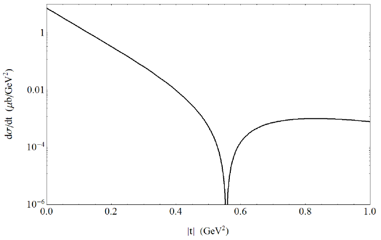
Figure 1: The contribution of $\omega$ and $\rho$-meson Regge trajectories to the differential cross section $d\sigma_{R}/dt$ for $f_{1}$ photoproduction for $|t|\leq 1{\rm GeV}^{2}$ at $s=10\ {\rm GeV}^{2}$ ($E_{\gamma}\simeq 4.6\ {\rm GeV}$ in lab frame).

The differential cross-section for $f_{1}$ photoproduction is shown in Fig. 1. As expected, it exhibits a strongly collimated peak at forward angles corresponding to $t$-channel meson exchange. In the physical region, where $t\leq 0$, the differential cross section scales approximately as $s^{-1-1.8|t|}$. Fig. 1 also exhibits an EXD zero at $|t|\simeq 0.55\ {\rm GeV}^{2}$.

It is instructive to compare this contribution to the one from the nucleon’s $s$- and $u$-channel Regge trajectory exchange. Since the Regge trajectory for the nucleon is $\alpha_{N}(t)\simeq-0.3+0.9\ t$ (the values for the slope and intercept are taken from the Ref. Collins:1977jy ), we expect that at large $s$, the differential cross section should decrease like $s^{-2.6}$. This suggests that for large $s$ exchange of the $\omega$ and $\rho$ Regge trajectories is dominant.

IV.4 $\omega$ ($\rho$) photoproduction

For the $\omega$ or $\rho^{0}$ meson photoproduction at high center of mass energies, the Regge trajectory exchange (from $\pi$, $\sigma$ and $f_{1}$ mesons) must also be taken into account. The single particle contributions that also include tensor mesons are considered in Ref. Oh:2003aw . We will only be interested in the contribution from the Regge trajectory corresponding to $f_{1}$ meson. This trajectory should be dominant, since the Regge trajectory for the pion is $\alpha_{\pi}(t)\simeq 0.0+0.8\ t$, therefore, the differential cross section will decrease as $s^{-2}$.

The contribution of the single-particle exchange to the $\omega$ photoproduction amplitude can be written as:

$${\cal M}_{\rm sp}=i\ e\ g_{f_{1}NN}\ g_{\gamma\omega f_{1}} \epsilon^{\mu\nu\alpha\beta}\ \epsilon^{*}_{\mu}(\gamma)\epsilon_{\nu}(\omega)\ p_{1\beta}\ \frac{1}{t-M^{2}_{f_{1}}}\ F_{f_{1}NN}(t)\ \bar{u}_{s^{\prime}}(q_{2})\gamma^{\alpha}\gamma^{5}u_{s}(q_{1})\ .$$ (93)

where $\epsilon_{\nu}(\omega)$ is the polarization of produced $\omega$ meson and

$$F_{f_{1}NN}(t)=\frac{1}{(1-t/M^{2}_{f_{1}})^{2}}\ .$$ (94)

In the unpolarized case, the differential cross section for the $\omega$-photoproduction is:

$$\frac{d\sigma^{\omega}_{f_{1}}}{dt} =\frac{A_{f}F^{2}_{f_{1}NN}(t)}{8(t-M^{2}_{f_{1}})^{2}}\bar{\Phi}_{s}(s,t)\ ,$$ (95)

where $A_{f}\equiv\alpha_{\rm em}\ g^{2}_{f_{1}NN}\ g^{2}_{\gamma\omega f_{1}}$ and

$$\bar{\Phi}_{s}(s,t)=\frac{M^{2}_{N}-u}{s-M^{2}_{N}}+\frac{(M^{2}_{\omega}-t)}{2M^{2}_{\omega}}\left[\frac{(M^{2}_{N}-u)(M^{2}_{N}+M^{2}_{\omega}-u)}{(s-M^{2}_{N})^{2}}+\frac{(s-M^{2}_{N}-M^{2}_{\omega})}{(s-M^{2}_{N})}+2M^{2}_{N}\frac{(M^{2}_{\omega}-t)}{(s-M^{2}_{N})}\right]\ .$$ (96)

Similarly, for $\rho$-photoproduction, we will have

$$\frac{d\sigma^{\rho}_{f_{1}}}{dt} =9\frac{d\sigma^{\omega}_{f_{1}}}{dt}\ ,$$ (97)

where we took into account that $M_{\omega}=M_{\rho}$ and $g_{\gamma\rho f_{1}}=3g_{\gamma\omega f_{1}}$.

To Reggeize the propagator, we make the following substitution:

$$\frac{1}{t-M^{2}_{f_{1}}}\ \rightarrow\ \frac{\pi\ \alpha^{\prime}_{f_{1}}}{2\ \Gamma(\alpha_{f_{1}}(t))}\ \eta(t)\left(\frac{s}{s_{0}}\right)^{\alpha_{f_{1}}(t)-1}\ ,$$ (98)

therefore, for large $s$,

$$\frac{d\sigma^{\omega}_{R}}{dt} =\pi^{2}A_{f}F^{2}_{f_{1}NN}(t)\ \frac{\left(1-\frac{t}{2M^{2}_{\omega}}\right)\alpha^{{}^{\prime}2}_{f_{1}}}{16\ \Gamma^{2}(\alpha_{f_{1}}(t))\cos^{2}\left(\frac{\pi\alpha_{f_{1}}(t)}{2}\right)}\ \left(\frac{s}{s_{0}}\right)^{2(\alpha_{f_{1}}(t)-1)}\ .$$ (99)

For $\rho$ photoproduction, the differential cross section will be $9$ times larger. Exchange of the $f_{1}$ Regge trajectory in $\omega$ or $\rho$ photoproduction leads to the same polarization structure as found previously for $f_{1}$ photoproduction via the exchange of the $\omega$ and $\rho$ Regge trajectories. This structure may be useful in trying to unravel the unknown Regge trajectory for the $f_{1}$ meson from measurements of polarized $\rho$ and $\omega$ photoproduction.

V Conclusions

Working in the theoretical framework of holographic QCD, we have calculated the couplings between vector and axial-vector mesons, the pion, and the photon which emerge from the 5D Chern-Simons term. Though interactions with the same structure were studied before (see, e.g. Ref. Kochelev:1999zf ), the advantage of holographic QCD is that it allows us to derive these interactions from a unified framework and determine all possible couplings between the mesons and the photon. Both holographic models we employ have only two free parameters, the gauge coupling strength ($g_{5}$ or $\lambda$) and the confinement scale ($1/z_{0}$ and $M_{KK}$), which are fixed by the $\rho$ meson mass and the pion decay constant.

To examine the experimental manifestation of these interactions, we studied the photoproduction of vector and axial vector mesons, such as $\omega$, $\rho$ and $f_{1}$, with special emphasis on $f_{1}$ photoproduction, as this is expected to have the clearest experimental signature. After determining the vertex functions $K_{\gamma Vf_{1}}(t)$ and couplings from holographic QCD, we borrowed the form factors and couplings involving the nucleon from the phenomenologically accepted models (including other holographic models) to calculate the scattering amplitudes at low energies (where single-particle exchange is a good approximation), then at large $s$ and small $|t|$, where we used Regge theory to substitute the single meson propagator with its Reggeized version. This yielded predictions for the differential cross sections for $f_{1}$ photoproduction in the $t$-channel. After considering other processes as well, we show that both the contribution from nucleon exchanges in the $u$- and $s$-channels and double photoproduction can be neglected. The primary contribution to the $f_{1}$ photoproduction comes from the exchange with $\omega$ and $\rho$ mesons. For large energies, the Regge trajectories of these mesons begin to dominate the process.

We consider both unpolarized and polarized cases and show that in the polarized case the polarization of the produced meson must be perpendicular to the polarization of the incident photon. This is specific to the “anomalous” type of interactions that contain a Levi-Civitá symbol. Precisely for this reason, polarized $\omega$ or $\rho$ photoproduction may be a very useful tool to determine the slope and intercept of the $f_{1}$ meson Regge trajectory.

Finally, we mention some interesting directions for future work. Our focus has been on hadronic couplings to the photon, it would be natural to generalize our work to include the electroweak gauge bosons $W^{\pm},Z^{0}$ as background fields and to compare to the results of Harvey:2007ca . In our treatment of photoproduction we have taken the nucleon couplings and form factors as determined from other phenomenological fits. It would be more consistent to calculate these in a holographic framework using previous results on the description of nucleons in string duals of QCD Hata:2007mb ; Hashimoto:2008zw ; Hong:2007ay . Our calculations have been done for $N_{f}=2$ and in the chiral limit of massless pions. The extensions to $N_{f}=3$ and to massive quarks are worth pursuing. Finally, it would be interesting to see if there are other photoproduction processes that can be used to further probe the types of couplings that we have analyzed here.

Note Added: As this work was being finished a preprint appeared which also considers photoproduction of $f_{1}$ mesons at JLab Kochelev:2009xz . Their predicted differential cross section differs from ours.

Appendix A Three- and four-point pseudo-Chern-Simons Couplings

A.1 The Hirn-Sanz model

We summarize the couplings resulting from the Chern-Simons action in the Sakai-Sugimoto and Hirn-Sanz models. A number of these couplings have been worked for $N_{f}=3$ in the Sakai-Sugimoto model Sakai:2005yt .

Recall the Chern-Simons action for the Hirn-Sanz model

$$S_{CS}=\frac{N_{c}}{24\pi^{2}}\int\left[\omega_{5}(L)-\omega_{5}(R)\right]\ ,$$ (100)

with

$$\omega_{5}(A) = \mathop{\rm tr}\left[AF^{2}+\frac{i}{2}A^{3}F-\frac{1}{10}A^{5}\right]$$ (101)

$$= \mathop{\rm tr}\left[A(dA)^{2}-\frac{3i}{2}A^{3}dA-\frac{3}{5}A^{5}\right]\ ,$$ (102)

where $L$ and $R$ are $U(N_{f})$-valued. The Chern-Simons (CS) action is only defined up to boundary terms. As in Sakai:2004cn , we assume that the action is initially written in a gauge where all gauge fields vanish at the (UV) boundary of the space. When we transform to $L_{z}=R_{z}=0$ gauge, we generate boundary terms of the form

$$S_{{\rm bdy}}=\frac{N_{c}}{24\pi^{2}}\int_{M^{4}}\left[\alpha_{4}(d\xi_{L}^{-1}\xi_{L},L)-\alpha_{4}(d\xi_{R}^{-1}\xi_{R},R)\right]\ ,$$ (103)

where $\alpha_{4}$ is

$$\alpha_{4}(V,A)=-\frac{i}{2}\mathop{\rm tr}\left(V(iAdA+idAA+A^{3})-\frac{1}{2}VAVA-V^{3}A\right)~{}.$$ (104)

(There is also a WZW-like term which yields 5- and higher-point couplings.) Writing $V=(L+R)/2$ and $A=(L-R)/2$ as usual, we note that only terms containing an odd number of $A$’s will survive in the action, giving

$$S_{CS}=S_{CS-3}+S_{CS-4}+S_{CS-5}\ ,$$ (105)

where

$$S_{CS-3} = \frac{N_{c}}{12\pi^{2}}\int\mathop{\rm tr}\left[A(dA)^{2}+VdAdV+VdVdA+A(dV)^{2}\right]\ ,$$ (106)

$$S_{CS-4} = -\frac{iN_{c}}{8\pi^{2}}\int\mathop{\rm tr}\left[\left(V^{2}A+AV^{2}\right)dV+VAVdV+V^{3}dA\right]+\left(V\leftrightarrow A\right)\ ,$$ (107)

$$S_{CS-5} = -\frac{N_{c}}{4\pi^{2}}\int\mathop{\rm tr}\left[V^{4}A+V^{2}A^{3}+3VAVA^{2}+\frac{1}{5}A^{5}\right]~{}$$ (108)

and similarly for the boundary terms from $\alpha_{4}$, which contribute exclusively photon-pion couplings. We now expand the new (gauge-transformed) fields $V_{\mu}$ and $A_{\mu}$, keeping only the vector source $\hat{V}$, the pion $\pi$, and the lightest (axial) vector meson states:

$$V_{\mu}(x,z) =\hat{V}_{\mu}(x)+\frac{i}{2f_{\pi}^{2}}[\pi,\partial_{\mu}\pi]+\rho_{\mu}(x)\psi_{\rho}(z)+\dots\ ,$$ (109)

$$A_{\mu}(x,z) =\alpha(z)\frac{1}{f_{\pi}}\partial_{\mu}\pi-i\frac{\alpha(z)}{f_{\pi}}[\hat{V}_{\mu},\pi]+a_{\mu}(x)\psi_{a_{1}}(z)+\dots\ ,$$ (110)

where we have defined $\xi_{R}(x)=\xi_{L}^{\dagger}(x)=e^{i\pi/f_{\pi}}$ and expanded to second order in the fields. Note that we have absorbed the normalizable pieces of the gauge transformations $\tilde{\xi}_{L}$ and $\tilde{\xi}_{R}$ into the definitions of the vector mesons. The story is almost identical for the Sakai-Sugimoto model, where there is a single gauge field $A_{\mu}$ which splits into axial and vector pieces, as discussed above. Boundary terms are generated by the presence of two UV boundaries (L and R) which can similarly be exchanged by parity. The terms living on the brane (not at the boundaries) thus differ by an overall factor of $1/2$ with respect to the Hirn-Sanz model terms given in 106.

We work with $N_{f}=2$, with generators of $U(2)$ normalized such that ${\rm Tr}T^{a}T^{b}=\delta^{ab}/2$ (for $a,b=0,1,2,3$). As has been noted before, the photon is generated by the EM current (35). The photon appears in overlap integrals as the (nonnormalizable) zero-momentum solution to the vector gauge field equations of motion – in this case, $\psi_{\gamma}=1$. Also, each occurrence of the photon field $\gamma_{\mu}$ in the tables below should be accompanied by a factor of the electromagnetic coupling $e$. We give the couplings in terms of overlap integrals between wavefunctions using the notation for Hirn-Sanz

$$I_{B^{\prime}CCD}=\int_{0}^{z_{0}}dz\psi_{B}^{\prime}\psi_{C}^{2}\psi_{D}~{},$$ (111)

and for Sakai-Sugimoto

$$I_{B^{\prime}CCD}=\frac{1}{2}\int_{-\infty}^{\infty}dz\psi_{B}^{\prime}\psi_{C}^{2}\psi_{D}~{}=\int_{0}^{\infty}dz\psi_{B}^{\prime}\psi_{C}^{2}\psi_{D}~{}.$$ (112)

Because the overall coefficient of bulk integrals in Sakai-Sugimoto differs by a factor of $1/2$ with respect to Hirn-Sanz, but the domain of integration is $(-\infty,\infty)$, this notation allows us to write the couplings in the two models in precisely the same form. The wavefunctions are normalized to yield the canonical kinetic terms in the Yang-Mills Lagrangian.

To use these tables to extract the listed couplings one should take the interaction term given in the second column, contract the Lorentz indices with $\epsilon^{\mu\nu\rho\sigma}$ and multiply by $N_{c}/48\pi^{2}$, then write the resulting interaction term as the coupling given in the first column times terms involving fields and derivatives and the Levi-Civita tensor, but no constants. For example, the $\rho-f_{1}-\gamma$ interaction is $-6I_{AV^{\prime}}(N_{c}/48\pi^{2})\epsilon^{\mu\nu\rho\sigma}f_{\mu}\partial_{\nu}\gamma_{\rho}\rho^{0}_{\sigma}$ which we rewrite as $g_{\gamma\rho f}\epsilon^{\mu\nu\rho\sigma}f_{\mu}\partial_{\nu}\gamma_{\rho}\rho^{0}_{\sigma}$ with $g_{\gamma\rho f}=-6I_{AV^{\prime}}(N_{c}/48\pi^{2})$. The numerical values of these couplings are given in the final two columns of the tables, computed in the HS and SS models, respectively. We fix the free parameters in both the Hirn-Sanz (HS) and Sakai-Sugimoto (SS) models using $m_{\rho}$ and $f_{\pi}$.

TABLE III: Three-point couplings.
g	Interaction $\times(N_{c}/48\pi^{2})^{-1}$	Value in HS	Value in SS
$g_{\gamma\rho f}$	$-6I_{AV^{\prime}}f_{\mu}\partial_{\nu}\gamma_{\rho}\rho^{0}_{\sigma}$	$-1.03$	$-0.95$
$g_{\gamma\gamma\pi}$	$2f_{\pi}^{-1}\gamma_{\mu}\partial_{\nu}\gamma_{\rho}\partial_{\sigma}\pi^{0}$	$-0.01f_{\pi}^{-1}$	$-0.01f_{\pi}^{-1}$
$g_{\gamma\rho a}$	$-2I_{AV^{\prime}}a_{\mu}^{a}\partial_{\nu}\gamma_{\rho}\rho_{\sigma}^{b}\delta_{ab}$	$-0.34$	$-0.32$
$g_{\gamma\rho\pi}$	$2I_{\pi^{\prime}V}f_{\pi}^{-1}\partial_{\mu}\pi^{a}\partial_{\nu}\gamma_{\rho}\rho_{\sigma}^{b}\delta_{ab}$	$-0.06f_{\pi}^{-1}$	$-0.06f_{\pi}^{-1}$
$g_{\gamma a\omega}$	$-6I_{AV^{\prime}}a_{\mu}^{0}\partial_{\nu}\gamma_{\rho}\omega_{\sigma}$	$-1.03$	$-0.95$
$g_{\gamma\pi\omega}$	$6I_{\pi^{\prime}V}f_{\pi}^{-1}\partial_{\mu}\pi^{0}\partial_{\nu}\gamma_{\rho}\omega_{\sigma}$	$-0.18f_{\pi}^{-1}$	$-0.18f_{\pi}^{-1}$
$g_{\pi af}$	$3I_{AA\pi^{\prime}}f_{\pi}^{-1}\partial_{\mu}\pi^{a}(\partial_{\nu}a_{\rho}^{b}f_{\sigma}-\partial_{\nu}f_{\sigma}a_{\rho}^{b})\delta_{ab}$	$-0.31f_{\pi}^{-1}$	$-0.26f_{\pi}^{-1}$
$g_{\gamma\omega f}$	$-2I_{AV^{\prime}}f_{\mu}\partial_{\nu}\gamma_{\rho}\omega_{\sigma}$	$-0.34$	$-0.32$
$g_{\omega\rho a}$	$-3I_{A^{\prime}VV}a_{\mu}^{a}(\partial_{\nu}\omega_{\rho}\rho_{\sigma}^{b}-\omega_{\rho}\partial_{\nu}\rho_{\sigma}^{b})\delta_{ab}$	$4.09$	$3.70$
$g_{\omega\rho\pi}$	$-3I_{\pi^{\prime}VV}f_{\pi}^{-1}\partial_{\mu}\pi^{a}(\partial_{\nu}\omega_{\rho}\rho_{\sigma}^{b}-\omega_{\rho}\partial_{\nu}\rho_{\sigma}^{b})\delta_{ab}$	$-0.52f_{\pi}^{-1}$	$-0.51f_{\pi}^{-1}$
$g_{\rho\rho f}$	$3I_{A^{\prime}VV}f_{\mu}\partial_{\nu}\rho_{\rho}^{a}\rho_{\sigma}^{b}\delta_{ab}$	$-4.09$	$-3.70$
$g_{\omega\omega f}$	$3I_{A^{\prime}VV}f_{\mu}\partial_{\nu}\omega_{\rho}\omega_{\sigma}$	$-4.09$	$-3.70$

The four-point couplings are

TABLE IV: Four-point couplings.
g	Interaction $\times(N_{c}/48\pi^{2})^{-1}$	Value in HS	Value in SS
$g_{\gamma\gamma\rho\pi}$	$-2I_{\pi V^{\prime}}f_{\pi}^{-1}\gamma_{\mu}\partial_{\nu}\gamma_{\rho}\pi^{a}\rho_{\rho}^{b}\epsilon^{ab3}$	$-0.06f_{\pi}^{-1}$	$-0.06f_{\pi}^{-1}$
$g_{\gamma\rho\rho f}$	$3I_{A^{\prime}VV}\rho_{\mu}^{a}\rho_{\nu}^{b}f_{\rho}\gamma_{\sigma}\epsilon^{ab3}$	$4.09$	$3.70$
$g_{\gamma\rho\omega a}$	$3I_{A^{\prime}VV}\gamma_{\mu}\rho_{\nu}^{a}a_{\rho}^{b}\omega_{\sigma}\epsilon^{ab3}$	$4.09$	$3.70$
$g_{\gamma\rho\omega\pi}$	$-3I_{\pi^{\prime}VV}f_{\pi}^{-1}\gamma_{\mu}(\partial_{\nu}\omega_{\rho}\pi^{a}\rho_{\sigma}^{b}-\pi^{a}\omega_{\rho}\partial_{\nu}\rho_{\sigma}^{b}+\partial_{\nu}\pi^{a}\omega_{\rho}\rho^{b}_{\sigma})\epsilon^{ab3}$	$0.52f_{\pi}^{-1}$	$0.51f_{\pi}^{-1}$
$g_{\gamma\pi\pi f}$	$3I_{A^{\prime}\pi\pi}f_{\pi}^{-2}\epsilon^{ab3}\partial_{\mu}\pi^{a}\partial_{\nu}\pi^{b}f_{\rho}\gamma_{\sigma}$	$-0.08f_{\pi}^{-2}$	$-0.07f_{\pi}^{-2}$
$g_{\gamma\pi af}$	$3I_{AA\pi^{\prime}}f_{\pi}^{-1}\gamma_{\mu}(\pi^{a}\partial_{\nu}a_{\rho}^{b}f_{\sigma}-\pi^{a}\partial_{\nu}f_{\sigma}a_{\rho}^{b}+\partial_{\nu}\pi^{a}a_{\rho}^{b}f_{\sigma})\epsilon^{ab3}$	$-0.31f_{\pi}^{-1}$	$-0.26f_{\pi}^{-1}$
$g_{\gamma\pi\pi\pi}$	$(f_{\pi}^{-3}/2)\partial_{\mu}\pi^{a}\partial_{\nu}\pi^{b}\partial_{\rho}\pi^{c}\gamma_{\sigma}\epsilon^{abc}$	$0.003f_{\pi}^{-3}$	$0.003f_{\pi}^{-3}$
$g_{\rho\rho\rho f}$	$I_{A^{\prime}VVV}f_{\mu}\rho_{\nu}^{a}\rho_{\rho}^{b}\rho_{\sigma}^{c}\epsilon^{abc}$	$9.52$	$8.42$
$g_{\omega\rho\rho a}$	$I_{A^{\prime}VVV}\rho_{\mu}^{a}\rho_{\nu}^{b}a_{\rho}^{c}\omega_{\sigma}\epsilon^{abc}$	$9.52$	$8.42$
$g_{\omega\rho\rho\pi}$	$I_{\pi^{\prime}VVV}f_{\pi}^{-1}\rho_{\mu}^{a}\rho_{\nu}^{b}\partial_{\rho}\pi^{c}\omega_{\sigma}\epsilon^{abc}$	$-1.03f_{\pi}^{-1}$	$-1.03f_{\pi}^{-1}$
$g_{\omega aaa}$	$I_{AAAV^{\prime}}a_{\mu}^{a}a_{\nu}^{b}a_{\rho}^{c}\omega_{\sigma}\epsilon^{abc}$	$3.78$	$2.93$
$g_{\omega\pi aa}$	$3I_{AA\pi V^{\prime}}f_{\pi}^{-1}a_{\mu}^{a}a_{\nu}^{b}\partial_{\rho}\pi^{c}\omega_{\sigma}\epsilon^{abc}$	$1.49f_{\pi}^{-1}$	$1.31f_{\pi}^{-1}$
$g_{\omega\pi\pi a}$	$3(I_{AV^{\prime}}+I_{A\pi\pi V^{\prime}})f_{\pi}^{-2}a_{\mu}^{a}\partial_{\nu}\pi^{b}\partial_{\rho}\pi^{c}\omega_{\sigma}\epsilon^{abc}$	$0.75f_{\pi}^{-2}$	$0.70f_{\pi}^{-2}$
$g_{\omega\pi\pi\pi}$	$(3I_{\pi V^{\prime}}-I_{V^{\prime}\pi\pi\pi})f_{\pi}^{-3}\partial_{\mu}\pi^{a}\partial_{\nu}\pi^{b}\partial_{\rho}\omega_{s}\pi^{c}\epsilon^{abc}$	$-0.07f_{\pi}^{-3}$	$-0.07f_{\pi}^{-3}$
$g_{\rho aaf}$	$I_{AAAV^{\prime}}f_{\mu}a_{\nu}^{a}a_{\rho}^{b}\rho_{\sigma}^{c}\epsilon^{abc}$	$3.79$	$2.93$
$g_{\rho\pi af}$	$-6I_{AA^{\prime}\pi V}f_{\pi}^{-1}\partial_{\mu}\pi^{a}a_{\nu}^{b}\rho_{\rho}^{c}f_{\sigma}\epsilon^{abc}$	$0.04f_{\pi}^{-1}$	$0.13f_{\pi}^{-1}$
$g_{\rho\pi\pi f}$	$3(I_{A^{\prime}V}+I_{A^{\prime}\pi\pi V})f_{\pi}^{-2}f_{\mu}\partial_{\nu}\pi^{a}\partial_{\rho}\pi^{b}\rho_{\sigma}^{b}\epsilon^{abc}$	$-0.42f_{\pi}^{-2}$	$-0.42f_{\pi}^{-2}$

Appendix B Single Nucleon Exchange Contribution to $f_{1}$ Photoproduction

The interactions relevant for nucleon exchange diagrams on Fig. 2 (when nucleon is proton) emerge from the following Lagrangians:

$${\cal L}_{\gamma pp}=-e\ \bar{\psi}_{N}\left[\gamma^{\mu}A_{\mu}-\frac{\kappa_{p}}{2M_{N}}\sigma_{\mu\nu}\partial^{\nu}A^{\mu}\right]\psi_{N}\ ,$$ (113)

$${\cal L}_{f_{1}NN}=g_{f_{1}NN}\ \bar{\psi}_{N}\left[f_{1\mu}-i\frac{\kappa_{f_{1}}}{2M_{N}}\gamma^{\nu}\partial_{\nu}f_{1\mu}\right]\gamma^{\mu}\gamma^{5}\psi_{N}\ ,$$

where $A_{\mu}$ describes electromagnetic field, $f_{1\mu}$ describes the isosinglet axial-vector meson field, $\kappa_{p}\simeq 1.79$ is the anomalous magnetic moment of the nucleon. Here, we will ignore $\kappa_{f_{1}}$ as well as $\kappa_{p}$, since these are $q/M_{N}$ suppressed. The value of the coupling $g_{f_{1}NN}=2.5\pm 0.5$ is fixed through the proton spin analysis Birkel:1995ct .

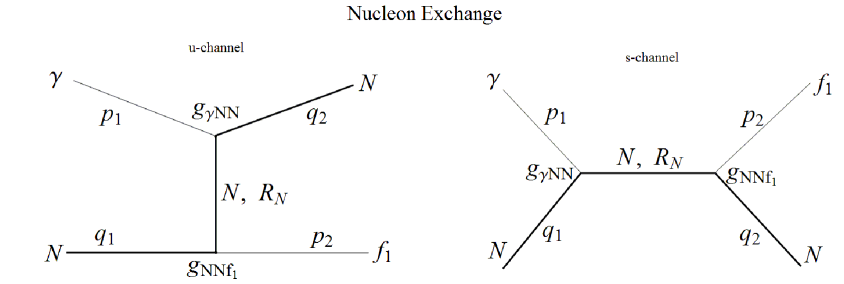
Figure 2: Photoproduction of $f_{1}$ meson in $u$- (left) and $s$- (right) channel correspondingly, via the exchange of either single nucleon or nucleon Regge trajectory.

The production amplitude in $u$- and $s$- channels can be written as:

$${\cal M}^{\mu\nu}_{u,s}=e\ g_{f_{1}NN}\ \bar{u}(q_{2})\left[\gamma^{\mu}\frac{/{\!\!\!}{q_{1}}-/{\!\!\!}{p_{2}}+M_{N}}{u-M^{2}_{N}}\gamma^{\nu}\gamma^{5}F_{N}(u)+\gamma^{\nu}\gamma^{5}\frac{/{\!\!\!}{p_{1}}+/{\!\!\!}{q_{1}}+M_{N}}{s-M^{2}_{N}}\gamma^{\mu}F_{N}(s)\right]u(q_{1})\ ,$$ (114)

where

$$F_{N}(u)=\frac{\Lambda^{4}_{N}}{\Lambda^{4}_{N}+(u-M^{2}_{N})^{2}}\ ,$$ (115)

and $\Lambda_{N}=0.5\ {\rm GeV}$ taken from the Ref. Oh:2003aw and references therein.

When $F_{N}(u)=F_{N}(s)=F$, it follows that $p^{\mu}_{1}{\cal M}^{\mu\nu}_{u,s}=0$ when $p^{2}_{1}=0$. In general, $F_{N}(u)\neq F_{N}(s)$ and the gauge invariance is broken (the term proportional to $\kappa_{p}$ won’t change the situation). The gauge invariance may be restored by redefining the interaction vertices. However, this shouldn’t significantly change the final results.

Without going into details, it suffices to show that in the limit, when $s\gg M^{2}_{N}$ and $t$ is fixed,

$$\frac{d\sigma_{N}}{dt}\simeq\frac{\alpha_{\rm em}g^{2}_{f_{1}NN}}{M^{4}_{N}}\ \left(\frac{\Lambda_{N}}{M_{N}}\right)^{8}\ \frac{1}{\tilde{s}^{6}}\sim\frac{0.001}{\tilde{s}^{6}}\ ,$$ (116)

where $\tilde{s}=s/M^{2}_{N}$. For comparison, in the same limit, the differential cross section corresponding to single $\omega$ and $\rho$ meson exchange is:

$$\frac{d\sigma_{V}}{dt}\sim\frac{1}{\pi}\left(\frac{r\ g_{\rho NN}\ eg_{\gamma\rho f_{1}}}{4M^{2}_{\rho}}\right)^{2}\left(\frac{\Lambda_{VNN}}{M_{N}}\right)^{8}\ \frac{1}{\tilde{s}^{4}}\sim\frac{0.1}{\tilde{s}^{4}}\ .$$ (117)

Summarizing, at large $s$ and fixed (small) $|t|$, the cross section corresponding to nucleon exchange decreases as $1/s^{6}$, and the meson contribution is absolutely dominant over the nucleon contribution.

Appendix C $f_{1}\rightarrow\rho^{0}+\gamma$

As a further check of the predictions of AdS/QCD for pseudo-Chern-Simons terms we use the couplings given in Table III to compute the rate and polarization structure for the decay $f_{1}\rightarrow\rho^{0}+\gamma$ . The interaction Lagrangian for this process is given in

$${\cal L}_{\gamma\rho^{0}f_{1}}=eg_{\gamma\rho f}\epsilon^{\mu\nu\lambda\rho}\partial_{\mu}A_{\nu}\rho_{\lambda}f_{1,\rho}\ .$$ (118)

For photon momentum $q$ and polarization vectors $\epsilon^{(\gamma)},\epsilon^{(f)}$ and $\epsilon^{(\rho)}$ for the photon, $f_{1}$ and $\rho$ respectively the decay amplitude is

$$i{\cal M}=ieg_{\gamma\rho f}\epsilon^{\mu\nu\alpha\beta}\bigl{(}iq_{\mu}\epsilon_{\nu}^{(\gamma)*}\bigr{)}\epsilon_{\alpha}^{(\rho)*}\epsilon_{\beta}^{(f)}$$ (119)

and leads to a decay rate

$$\Gamma(f_{1}\rightarrow\rho^{0}+\gamma)=\frac{\alpha g_{\gamma\rho f}^{2}}{3}\frac{E_{\gamma}^{3}}{m_{\rho}^{2}}\biggl{(}1+\frac{m_{\rho}^{2}}{m_{f}^{2}}\biggr{)}$$ (120)

where $E_{\gamma}=(m_{f}^{2}-m_{\rho}^{2})/2m_{f}$ is the energy of the final state photon in the $f_{1}$ rest frame. Comparison to the measured rate pdg

$$\Gamma_{\rm exp}(f_{1}\rightarrow\rho^{0}+\gamma)=1.33~{}\pm.37~{}{\rm MeV}$$ (121)

requires that $|g_{\gamma\rho f}|=1.7~{}\pm.4$ which should be compared with the value of $g_{\gamma\rho f}\simeq-1$ given in Table III of Appendix A. The agreement is not spectacular, but is much better than an old quark model calculation of this process Babcock . We note that if we use $g_{5}=2\pi$ in the Hirn-Sanz model as determined from the vector-vector two point function rather then the value $g_{5}=4.91$ determined from fitting to $f_{\pi}$ we obtain $g_{\gamma\rho f}=-1.68$.

A study of the polarization structure shows that the ratio for the decay of longitudinal to transverse $\rho$ mesons is $\Gamma_{\rm long}/\Gamma_{\rm trans}=m_{f}^{2}/m_{\rho}^{2}\simeq 2.7$. Unfortunately the experimental situation appears to be unclear. The papers Coffman ; Amelin give conflicting results for the polarization structure. Our results are in rough agreement with the results of Amelin .

References

- (1) A. Donnachie and P. V. Landshoff, “Total cross-sections,” Phys. Lett. B 296, 227 (1992).
- (2) J. M. Maldacena, “The large N limit of superconformal field theories and supergravity,” Adv. Theor. Math. Phys. 2, 231 (1998) [Int. J. Theor. Phys. 38, 1113 (1999)].
- (3) S. S. Gubser, I. R. Klebanov and A. M. Polyakov, “Gauge theory correlators from non-critical string theory,” Phys. Lett. B 428, 105 (1998).
- (4) E. Witten, “Anti-de Sitter space and holography,” Adv. Theor. Math. Phys. 2, 253 (1998).
- (5) T. Sakai and S. Sugimoto, “Low energy hadron physics in holographic QCD,” Prog. Theor. Phys. 113, 843 (2005) [arXiv:hep-th/0412141].
- (6) T. Sakai and S. Sugimoto, “More on a holographic dual of QCD,” Prog. Theor. Phys. 114, 1083 (2005) [arXiv:hep-th/0507073].
- (7) J. Erlich, E. Katz, D. T. Son and M. A. Stephanov, “QCD and a holographic model of hadrons,” Phys. Rev. Lett. 95, 261602 (2005) [arXiv:hep-ph/0501128].
- (8) L. Da Rold and A. Pomarol, “Chiral symmetry breaking from five dimensional spaces,” Nucl. Phys. B 721, 79 (2005); “The scalar and pseudoscalar sector in a five-dimensional approach to chiral symmetry breaking,” JHEP 0601, 157 (2006).
- (9) J. Polchinski and M. J. Strassler, “Deep inelastic scattering and gauge/string duality,” Phys. Rev. Lett. 88, 031601 (2002); JHEP 0305, 012 (2003).
- (10) S. J. Brodsky and G. F. de Téramond, “Light-front hadron dynamics and AdS/CFT correspondence,” Phys. Lett. B 582, 211 (2004); G. F. de Teramond and S. J. Brodsky, “The hadronic spectrum of a holographic dual of QCD,” Phys. Rev. Lett. 94, 201601 (2005).
- (11) C. Csaki, M. Reece and J. Terning, “The AdS/QCD Correspondence: Still Undelivered,” arXiv:0811.3001 [hep-ph].
- (12) S. K. Domokos and J. A. Harvey, “Baryon number-induced Chern-Simons couplings of vector and axial-vector mesons in holographic QCD,” Phys. Rev. Lett. 99, 141602 (2007) [arXiv:0704.1604 [hep-ph]].
- (13) M. Harada and C. Sasaki, “A novel spectral broadening from vector–axial-vector mixing in dense matter,” arXiv:0902.3608 [hep-ph].
- (14) J. A. Harvey, C. T. Hill and R. J. Hill, “Standard Model Gauging of the Wess-Zumino-Witten Term: Anomalies, Global Currents and pseudo-Chern-Simons Interactions,” Phys. Rev. D 77, 085017 (2008) [arXiv:0712.1230 [hep-th]].
- (15) J. A. Harvey, C. T. Hill and R. J. Hill, “Anomaly mediated neutrino-photon interactions at finite baryon density,” Phys. Rev. Lett. 99, 261601 (2007) [arXiv:0708.1281 [hep-ph]].
- (16) H. Hata, T. Sakai, S. Sugimoto and S. Yamato, “Baryons from instantons in holographic QCD,” arXiv:hep-th/0701280.
- (17) K. Hashimoto, T. Sakai and S. Sugimoto, “Holographic Baryons : Static Properties and Form Factors from Gauge/String Duality,” Prog. Theor. Phys. 120, 1093 (2008) [arXiv:0806.3122 [hep-th]].
- (18) D. K. Hong, M. Rho, H. U. Yee and P. Yi, “Dynamics of Baryons from String Theory and Vector Dominance,” JHEP 0709, 063 (2007) [arXiv:0705.2632 [hep-th]].
- (19) J. Hirn and V. Sanz, “Interpolating between low and high energy QCD via a 5D Yang-Mills model,” JHEP 0512, 030 (2005).
- (20) E. Witten, “Anti-de Sitter space, thermal phase transition, and confinement in gauge theories,” Adv. Theor. Math. Phys. 2, 505 (1998) [arXiv:hep-th/9803131].
- (21) H. R. Grigoryan and A. V. Radyushkin, “Form Factors and Wave Functions of Vector Mesons in Holographic QCD,” Phys. Lett. B 650, 421 (2007) [arXiv:hep-ph/0703069].
- (22) H. R. Grigoryan and A. V. Radyushkin, “Pion in the Holographic Model with 5D Yang-Mills Fields,” Phys. Rev. D 78, 115008 (2008) [arXiv:0808.1243 [hep-ph]].
- (23) D. Gazit and H. U. Yee, “Weak-Interacting Holographic QCD,” Phys. Lett. B 670, 154 (2008) [arXiv:0807.0607 [hep-th]].
- (24) D. T. Son and M. A. Stephanov, “QCD and dimensional deconstruction,” Phys. Rev. D 69, 065020 (2004) [arXiv:hep-ph/0304182].
- (25) C. T. Hill and C. K. Zachos, “Dimensional deconstruction and Wess-Zumino-Witten terms,” Phys. Rev. D 71, 046002 (2005); C. T. Hill, “Exact equivalence of the D = 4 gauged Wess-Zumino-Witten term and the D = 5 Yang-Mills Chern-Simons term,” Phys. Rev. D 73, 126009 (2006); C. T. Hill, “Anomalies, Chern-Simons terms and chiral delocalization in extra dimensions,” Phys. Rev. D 73, 085001 (2006).
- (26) P. D. B. Collins, “An Introduction To Regge Theory And High-Energy Physics,” Cambridge 1977, 445p.
- (27) T. H. Bauer, R. D. Spital, D. R. Yennie and F. M. Pipkin, “The Hadronic Properties Of The Photon In High-Energy Interactions,” Rev. Mod. Phys. 50, 261 (1978) [Erratum-ibid. 51, 407 (1979)].
- (28) Y. s. Oh, A. I. Titov and T. S. H. Lee, “Electromagnetic production of vector mesons at low energies,” arXiv:nucl-th/0004055.
- (29) H. Haberzettl, C. Bennhold, T. Mart and T. Feuster, “Gauge-invariant tree-level photoproduction amplitudes with form factors,” Phys. Rev. C 58, 40 (1998) [arXiv:nucl-th/9804051].
- (30) C. Savkli, F. Tabakin and S. N. Yang, “Multipole analysis of spin observables in vector meson photoproduction,” Phys. Rev. C 53, 1132 (1996); C. G. Fasano, F. Tabakin and B. Saghai, “Spin observables at threshold for meson photoproduction,” Phys. Rev. C 46, 2430 (1992).
- (31) M. Guidal, J. M. Laget and M. Vanderhaeghen, “Pion and kaon photoproduction at high energies: Forward and intermediate angles,” Nucl. Phys. A 627, 645 (1997).
- (32) A. C. Irving and R. P. Worden, “Regge Phenomenology,” Phys. Rept. 34 (1977) 117.
- (33) A. V. Barnes et al., “Pion Charge Exchange Scattering At High-Energies,” Phys. Rev. Lett. 37, 76 (1976).
- (34) N. I. Kochelev, D. P. Min, Y. s. Oh, V. Vento and A. V. Vinnikov, “A new anomalous trajectory in Regge theory,” Phys. Rev. D 61, 094008 (2000) [arXiv:hep-ph/9911480].
- (35) N. I. Kochelev, M. Battaglieri and R. De Vita, “Exclusive photoproduction of meson off proton in the JLab kinematics,” arXiv:0903.5369 [nucl-th].
- (36) M. Birkel and H. Fritzsch, “The Nucleon Spin and the Mixing of Axial Vector Mesons,” Phys. Rev. D 53, 6195 (1996) [arXiv:hep-ph/9511424].
- (37) Y. s. Oh, N. I. Kochelev, D. P. Min, V. Vento and A. V. Vinnikov, “Anomalous f1 exchange in vector meson photoproduction asymmetries,” Phys. Rev. D 62, 017504 (2000) [arXiv:hep-ph/0001209]. A. Donnachie and P. V. Landshoff, Nucl. Phys. B 231, 189 (1984); Nucl. Phys. B 244, 322 (1984); Nucl. Phys. B 267, 690 (1986); Phys. Lett. B 348, 213 (1995) [arXiv:hep-ph/9411368].
- (38) Y. s. Oh and T. S. H. Lee, “rho meson photoproduction at low energies,” Phys. Rev. C 69, 025201 (2004) [arXiv:nucl-th/0306033].
- (39) C. Amsler et al. [Particle Data Group], “Review of particle physics,” Phys. Lett. B 667, 1 (2008).
- (40) D. Coffman et al. [MARK-III Collaboration], “Study of The Doubly Radiative Decay J / psi gamma gamma rho0,” Phys. Rev. D 41, 1410 (1990).
- (41) D. V. Amelin et al., “Study Of The Decay F1 (1285) Rho0 (770) Gamma,” Z. Phys. C 66, 71 (1995).
- (42) J. Babcock and J. L. Rosner, “Radiative Transitions Of Low Lying Positive-Parity Mesons,” Phys. Rev. D 14, 1286 (1976).