Quantum Hall Effect in Biased Bilayer Graphene

Abstract

We numerically study the quantum Hall effect in biased bilayer graphene based on a tight-binding model in the presence of disorder. Integer quantum Hall plateaus with quantized conductivity $\sigma_{xy}=\nu e^{2}/h$ (where $\nu$ is any integer) are observed around the band center due to the split of the valley degeneracy by an opposite voltage bias added to the two layers. The central ($n=0$) Dirac Landau level is also split, which leads to a pronounced $\nu=0$ plateau. This is consistent with the opening of a sizable gap between the valence and conduction bands. The exact spectrum in an open system further reveals that there are no conducting edge states near zero energy, indicating an insulator state with zero conductance. Consequently, the resistivity should diverge at Dirac point. Interestingly, the $\nu=0$ insulating state can be destroyed by disorder scattering with intermediate strength, where a metallic region is observed near zero energy. In the strong disorder regime, the Hall plateaus with nonzero $\nu$ are destroyed due to the float-up of extended levels toward the band center and higher plateaus disappear first.

I I. Introduction

The discovery of an unusual quantum Hall effect (QHE) in bilayer graphene has stimulated great interest in the study of the electronic transport properties of this new material K. S. Novoselov ; R. V. Gorbachev ; S. V. Morozov ; E. A. Henriksen ; E. McCann ; J. Nilsson ; J. G. Checkelsky ; Y. Hasegawa ; D. A. Abanin ; E. V. Gorbar ; H. Min ; E. V. Castro ; R. Ma . At low energies and long wavelengths, the electrons in bilayer graphene can be described in terms of massive, chiral, Dirac particles. While previous studies have focused on unbiased and thus gapless bilayer graphene, recent experimental and theoretical studies T. Ohta ; Castro ; Oostinga ; F.Guinea ; Min ; McCann have revealed some interesting aspects of biased bilayer graphene. It has been shown that an electronic gap between the valence and conduction bands opens up at the Dirac point and the low energy band acquires a Mexican hat dispersion relation by changing the density of charge carriers in the layers through the application of an external field or by chemical doping, which creates a potential difference between the layers. The presence of the potential bias transforms the bilayer graphene into the only known semiconductor with a tunable energy gap and may open a way for developing photodetectors and lasers tunable by the electric field effect.

Under strong perpendicular magnetic field, experimental results have shown that biased bilayer graphene exhibits a pronounced plateau at zero Hall conductivity $\sigma_{xy}$=0, which is absent in the unbiased case and can only be understood as due to the opening of a sizable gap between the valence and conduction bands Castro . Tight-binding calculations have shown that the existence of such a gap can have a significant effect on the Landau level (LL) spectrum McCann ; Castro . While disorder effect is known to be crucial in the conventional QHE systems, in-depth understanding of the properties of the QHE in the presence of disorder in biased bilayer graphene is still absent and hence greatly needed.

In this work, we carry out a numerical study of the QHE in biased bilayer graphene in the presence of disorder based upon a tight-binding model. The Hall conductivity near the band center exhibits a sequence of plateaus at $\sigma_{xy}=\nu e^{2}/h$ where $\nu$ is an integer, as in the conventional QHE systems. The $\nu=0$ plateau is robust with its width proportional to the strength of bias, which is consistent with the experimental observation. We further investigate the effect of random disorder on the QHE by calculating the Thouless number Edwards . Interestingly, at an intermediate disorder strength, the energy gap around $E_{f}=0$ disappears, which destroys the $\nu=0$ plateau, and the system undergoes a transition to a metallic state. In the strong-disorder (or weak-magnetic-field) regime, the QHE plateaus around the band center can be destroyed due to the float-up of extended levels toward the band center. The $\nu=\pm 2$ plateaus are the most stable ones, which disappear last. Furthermore, we have also calculated the energy spectrum for an open system (cylindric geometry), and performed numerically a Laughlin’s gauge experiment Laughlin ; Halperin by adiabatically inserting flux quantum to directly probe the quantum transport near the sample edges. No conducting edge states are observed in the $\nu=0$ energy gap, suggesting an insulating state with divergent resistivity.

The paper is organized as follows. In Sec. II, we introduce the model Hamiltonian and formulas for the calculation. In Sec. III, numerical results based on exact diagonalization and transport calculations are presented. Sec. IV concludes with a summary.

II II. The tight-binding model of biased bilayer graphene

We consider a bilayer graphene sample consisting of two coupled hexagonal lattices including inequivalent sublattices $A$, $B$ on the bottom layer and $\widetilde{A}$, $\widetilde{B}$ on the top layer. The two layers are arranged in the AB (Bernal) stacking S. B. Trickey ; K. Yoshizawa , where $B$ atoms are located directly below $\widetilde{A}$ atoms, and $A$ atoms are the centers of the hexagons in the other layer. Here, the in-plane nearest-neighbor hopping integral between $A$ and $B$ atoms or between $\widetilde{A}$ and $\widetilde{B}$ atoms is denoted by $\gamma_{AB}=\gamma_{\widetilde{A}\widetilde{B}}=\gamma_{0}$. For the interlayer coupling, we take into account the largest hopping integral between a $B$ atom and the nearest $\widetilde{A}$ atom $\gamma_{\widetilde{A}B}=\gamma_{1}$, and the smaller hopping integral between an $A$ atom and three nearest $\widetilde{B}$ atoms $\gamma_{A\widetilde{B}}=\gamma_{3}$. The values of these hopping integrals are taken to be $\gamma_{0}=3.16$ eV, $\gamma_{1}=0.39$ eV, and $\gamma_{3}=0.315$ eV, the same as in Ref. R. Ma .

We assume that each monolayer graphene has totally $L_{y}$ zigzag chains with $L_{x}$ atomic sites on each chain Sheng . The size of the sample will be denoted as $N=L_{x}\times L_{y}\times L_{z}$, where $L_{z}=2$ is the number of graphene monolayers stacked along the $z$ direction. In the presence of an applied magnetic field perpendicular to the plane of the biased bilayer graphene, the lattice model in real space can be written the following form R. Ma :

$$H = -\gamma_{0}(\sum\limits_{\langle ij\rangle}e^{ia_{ij}}c_{i}^{\dagger}c_{j}+\sum\limits_{\langle ij\rangle}e^{ia_{ij}}\widetilde{c}_{i}^{\dagger}\widetilde{c}_{j})$$ (1)

$$- \gamma_{1}\sum\limits_{\langle ij\rangle_{1}}e^{ia_{ij}}c_{jB}^{\dagger}\widetilde{c}_{i\widetilde{A}}-\gamma_{3}\sum\limits_{\langle ij\rangle_{3}}e^{ia_{ij}}c_{iA}^{\dagger}\widetilde{c}_{j\widetilde{B}}+h.c.$$

$$+ \sum\limits_{i}(w_{i}+\epsilon_{1})c_{i}^{\dagger}c_{i}+(w_{i}+\epsilon_{2})\widetilde{c}_{i}^{\dagger}\widetilde{c}_{i},$$

where $c_{i}^{\dagger}$($c_{iA}^{\dagger}$), $c_{j}^{\dagger}$($c_{jB}^{\dagger}$) are creating operators on $A$ and $B$ sublattices in the bottom layer, and $\widetilde{c}_{i}^{\dagger}$($\widetilde{c}_{i\widetilde{A}}^{\dagger}$), $\widetilde{c}_{j}^{\dagger}$($\widetilde{c}_{j\widetilde{B}}^{\dagger}$) are creating operators on $\widetilde{A}$ and $\widetilde{B}$ sublattices in the top layer. The sum $\sum_{\langle ij\rangle}$ denotes the intralayer nearest-neighbor hopping in both layers, $\sum_{\langle ij\rangle_{1}}$ stands for interlayer hopping between the $B$ sublattice in the bottom layer and the $\widetilde{A}$ sublattice in the top layer, and $\sum_{\langle ij\rangle_{3}}$ stands for the interlayer hopping between the $A$ sublattice in the bottom layer and the $\widetilde{B}$ sublattice in the top layer, as described above. For the biased system the two layers gain different electrostatic potentials, and the corresponding energy difference is given by $\Delta_{g}=\epsilon_{2}-\epsilon_{1}$ where $\epsilon_{1}=-\frac{1}{2}\Delta_{g}$, and $\epsilon_{2}=\frac{1}{2}\Delta_{g}$. For illustrative purpose, a relatively large asymmetric potential $\Delta_{g}=0.05\gamma_{0}$ is assumed. $w_{i}$ is a random disorder potential uniformly distributed in the interval $w_{i}\in[-W/2,W/2]\gamma_{0}$. The magnetic flux per hexagon $\phi=\sum_{{\small{\mbox{\hexagon}}}}a_{ij}=\frac{2\pi}{M}$ is proportional to the strength of the applied magnetic field $B$, where $M$ is assumed to be an integer.

III III. Results and Discussion

The Hall conductivity $\sigma_{xy}$ can be calculated by using the Kubo formula through exact diagonalization of the system Hamiltonian R. Ma . In Fig. 1, the Hall conductivity $\sigma_{xy}$ near the band center is plotted as a function of electron Fermi energy $E_{f}$ for a clean sample ($W=0$) of size $N=96\times 24\times 2$ with magnetic flux $\phi=\frac{2\pi}{48}$, for biased and unbiased cases. Since the Hall conductivity is antisymmetric about zero energy, we show it mainly in the negative energy region. As we can see, in the unbiased case, the Hall conductivity exhibits a sequence of plateaus at $\sigma_{xy}=\nu e^{2}/h$, where $\nu=kg_{s}$ with $k$ an integer and $g_{s}=2$ due to double-valley degeneracy E. McCann ; Sheng (the spin degeneracy will contribute an additional factor $2$, which is omitted here). The transition from the $\nu=-2$ plateau to $\nu=2$ plateau is continuous without a $\nu=0$ plateau appearing in between, so that a step of height $4e^{2}/h$ occurs at the neutrality point. However, when a bias is applied, the valley degeneracy is lifted due to the different projection natures in the two layers of the LL states in the $K$ and $K^{\prime}$ valleys. The valley asymmetry has a strong effect on the LLs near zero energy, where the charge imbalance is saturated. As a consequence, the Hall conductivity is quantized as $\sigma_{xy}=\nu e^{2}/h$, where $\nu=kg_{s}$ with $k$ an integer and $g_{s}=1$ for each LL due to the split of double-valley degeneracy McCann . With each additional LL being occupied, the total Hall conductivity is increased by $e^{2}/h$. Around the particle-hole symmetric point $E_{f}=0$, a pronounced plateau with $\sigma_{xy}=0$ is found, which can only be understood as due to the opening of sizable gap, $\Delta_{g}$, between the valence and conductance bands. The emerged zero Hall plateau is accompanied by a huge peak in the longitudinal resistivity $\rho_{xx}$, indicating an insulating state. This behavior has been observed experimentally Castro . It implies that a diverging $\rho_{xx}$ at the particle-hole symmetric point $E_{f}=0$, in striking contrast to all the other Hall plateaus, where $\rho_{xx}$ vanishes as same as in ordinary QHE.

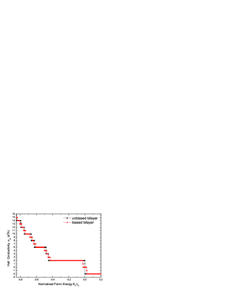
Figure 1: Hall conductivity near the band center of unbiased and biased bilayer graphene with $\phi=\frac{2\pi}{48}$ . The disorder strength and sample size are set to $W=0$ and $N=96\times 24\times 2$. Here, the spin degree of freedom has been omitted.

Now we study the effect of random disorder on the QHE around the band center in the biased bilayer graphene based upon the calculation of the Thouless number. In Fig. 2, the Hall conductivity $\sigma_{xy}$ and Thouless number $g$ around the band center are shown as functions of $E_{f}$ for three different disorder strengths and a relatively weak magnetic flux $\phi=\frac{2\pi}{48}$. In Fig. 2a, the calculated $\sigma_{xy}$ and Thouless number $g$ at a weak-disorder strength $W=0.2$ are plotted. Clearly, each valley in the Thouless number corresponds to a Hall plateau and each peak corresponds to a critical point between two neighboring Hall plateaus. We will call the central valley at $E_{f}=0$ the $\nu=0$ valley, the first one just above (below) it the $\nu=-1$ ($\nu=1$) valley, the second one the $\nu=-2$ ($\nu=2$) valley, and so on, as same as the Hall plateaus. In Fig. 2b, the Hall conductivity $\sigma_{xy}$ and Thouless number $g$ for a relatively strong-disorder strength $W=0.6$ are plotted. We see that the plateaus with $\pm 2$, $\pm 6$ and $\pm 10$ remain well quantized, and the other plateaus become indiscernible, because of their relatively small plateau widths. With increasing $W$, higher valleys in the Thouless number $g$ (with larger $|\nu|$) are destroyed first, indicating the destruction of the corresponding higher Hall plateau states. When $W=2.0$, all the plateaus except for the $\nu=\pm 2$ ones are destroyed (see Fig. 2c). The last two plateaus $\nu=\pm 2$ eventually disappear around $W\sim 3.2$. Thus we observed that the destruction of the QHE states near the band center are due to the float-up of extended levels toward zero energy.

In Fig. 3a, we show the Hall conductivity $\sigma_{xy}$ as a function of $E_{f}$ for a relatively strong magnetic flux $\phi=\frac{2\pi}{12}$ and three different system sizes $N=24\times 12\times 2$, $N=48\times 24\times 2$, $N=96\times 24\times 2$ at disorder strength $W=2.0$. We can see that at this disorder strength, the transition from $\nu=-2$ plateau to $\nu=2$ plateau becomes continuous. With increasing the system size, the width of the plateau $\nu=\pm 2$ remains nearly unchanged. The region around the zero energy of Fig. 3a is enlarged in Fig. 3b. For comparison, we also show the results for the unbiased case, which clearly demonstrate the continuous behavior between the $\nu=-2$ plateau to the $\nu=2$ plateau in both cases. This behavior indicates a metallic state occurs around zero energy, which is essentially caused by the strong coupling between the two Dirac LLs due to disorder scattering.

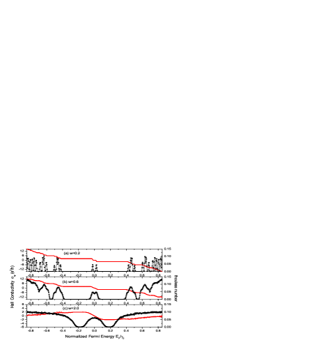
Figure 2: Calculated Thouless number and Hall conductivity for $\phi=\frac{2\pi}{48}$ and three different disorder strengths, which are averaged over 400 disorder configurations. Here, the sample sizes are taken to be $N=96\times 48\times 2$ and $N=96\times 24\times 2$ in the calculations of the Thouless number and the Hall conductivity, respectively.

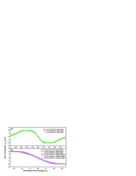
Figure 3: Calculated Hall conductivity for biased and unbiased bilayer graphene with magnetic flux $\phi=\frac{2\pi}{12}$ at disorder strength $W=2.0$ for three different system sizes.

We now investigate the evolution of the edge states in an infinitesimal electric field by performing the Laughlin’s gauge experiment Laughlin ; Halperin . A periodic boundary condition in the $y$ direction and an open boundary condition in the $x$ direction are imposed to the system. The system can thus be considered as a cylinder. When the flux $\theta_{y}(t)$ threading the cylinder is adiabatically turned on from $\theta_{y}(0)=0$ to $\theta_{y}(t)$=2$\pi$, which is equivalent to applying a weak electric field along the $y$ direction

$$E_{y}(t)=-\frac{1}{L_{y}}\frac{\partial\theta(t)}{\partial t}$$

. By diagonalizing the Hamiltonian Eq.(1) under the open boundary condition along the $x$-axis, at 200 different $\theta_{y}$, the eigenenergies $E_{n}$ of the system are obtained. Fig. 4a shows the calculated energy spectrum as a function of $\theta_{y}$ for a clean sample ($W=0$) at system size $N=96\times 24\times 2$. Note that $\theta_{y}=0$ and $\theta_{y}$=2$\pi$ are equivalent, as the system hamiltonian is periodic H($\theta_{y}=0$)=H($\theta_{y}$=2$\pi$). We first examine the energy spectrum corresponding to the $\nu=-2$ QHE plateau. We observe that with changing $\theta_{y}$, the energy levels in the plateau region cross each other, which correspond to two conducting edge channels in accordance with the quantized Hall effect. For example, we choose Fermi energy $E_{f}=0.1\gamma_{0}$. For $\theta_{y}=0$, in the ground state, all the single particle states below $E_{f}$ are occupied, whereas unoccupied above $E_{f}$. Upon insertion of the flux quantum, the two occupied states below $E_{f}$ are pumped onto states above $E_{f}$ indicated by the arrow, which causes two electrons transferred across from one edge to the other, corresponding to the quantized Hall conductivity with $\sigma_{xy}=2e^{2}/h$, as shown in Fig. 4b. However, there are no such conducting edge states near $E_{f}=0.0$, where the $\nu=0$ plateau is found. Clearly, a true spectrum gap shows up corresponding to a trivial insulating phase, which results in zero net charge transfer, and the current carried around the ribbon loop is zero.

Now we consider the disorder effect. Fig. 5a shows the results for a randomly chosen disorder configuration for $W=2.0$ at system size $N=96\times 24\times 2$. We can see that the energy gap around $E_{f}=0$ disappears. This behavior indicates that the transition from $\nu=-2$ plateau to $\nu=2$ plateau becomes continuous, as shown in Fig. 5b. In contrast, if we choose an arbitrary Fermi energy in the $\nu=\pm 2$ plateau regions, e.g., $E_{f}=0.16\gamma_{0}$, there are always two electrons transferred across from one edge to the other. Before the $\nu=2$ plateau is destroyed by the disorder, the $E_{f}=0$ point becomes metallic.

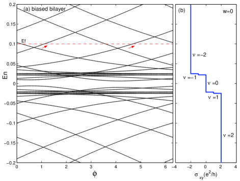
Figure 4: (a) Energy levels of biased bilayer graphene with an open boundary in the $x$ direction, as a function of the twisted boundary phase $\theta_{y}$ in the $y$ direction. (b) Hall conductivity near the band center for $W=0$. Here $\phi=\frac{2\pi}{48}$ and $N=96\times 24\times 2$.

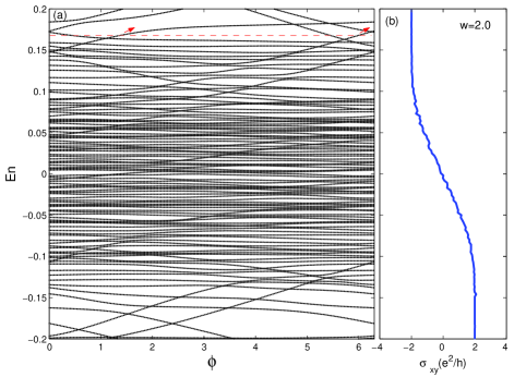
Figure 5: (a)Energy levels of unbiased bilayer graphene as a function of twisted phase $\theta_{y}$. (b) (b) Hall conductivity near the band center for $W=0$. Here $\phi=\frac{2\pi}{48}$ and $N=96\times 24\times 2$.

IV IV. Summary

In summary, we have numerically investigated the QHE in biased bilayer graphene based on tight-binding model in the presence of disorder. The experimentally observed unconventional QHE is reproduced near the band center, where the Hall conductivity is quantized as $\sigma_{xy}=\nu e^{2}/h$ with $\nu$ being any integer, including $\nu=0$. The $\nu=0$ plateau around $E_{f}=0$ is due to the opening of sizable gap between the valence and conductance bands, which is absent in the unbiased case. By performing numerically a laughlin’s gauge experiment, we have found that there are no conducting edge states in the $\nu=0$ plateau region, in contrast to the $\nu\neq 0$ plateaus, where energy levels across each other, resulting in charge transfer between the edges and charge accumulation at the edges. However, at an intermediate disorder strength, the energy gap around $E_{f}=0$ disappears, which indicates that the transition from $\nu=-2$ plateau to $\nu=2$ plateau becomes continuous, in agreement with the calculated results of the Hall conductivity. Furthermore, we show that with increasing disorder strength, the Hall plateaus can be destroyed through the float-up of extended levels toward the band center and higher plateaus disappear first. At a strong-critical-disorder strength $W=W_{c}=3.2$, the most stable QHE states with $\nu=\pm 2$ eventually disappear, which indicates a transition of all the QHE phases into an insulating phase.

Acknowledgment: This work is supported by the US DOE grant DE-FG02-06ER46305 (LJZ, DNS), the NSF grant DMR-0605696 (RM, DNS). We thank the KITP for partial support through the NSF grant PHY05-51164. We also thank the partial support from the State Scholarship Fund from the China Scholarship Council, the Scientific Research Foundation of Graduate School of Southeast University of China (RM), the doctoral foundation of Chinese Universities under grant No. 20060286044(ML), the National Basic Research Program of China under grant Nos.: 2007CB925104 and 2009CB929504 (LS), and the NSF of China grant No.: 10874066 (LS).

References

- (1) K. S. Novoselov, E. McCann, S. V. Morozov, V. I. Falko, M. I. Katsnelson, U. Zeitler, D. Jiang, F. Schedin, and A. K. Geim, Nat. Phys. 2, 177 (2006).
- (2) R. V. Gorbachev, F. V. Tikhonenko, A. S. Mayorov, D.W. Horsell, and A. K. Savchenko, Phys. Rev. Lett. 98, 176805 (2007).
- (3) S. V. Morozov, K. S. Novoselov, M. I. Katsnelson, F. Schedin, D. C. Elias, J. A. Jaszczak, and A. K. Geim, Phys. Rev. Lett. 100, 016602 (2008).
- (4) E. A. Henriksen, Z. Jiang, L. C. Tung, M. E. Schwartz, M. Takita, Y. J. Wang, P. Kim, and H. L. Stormer, Phys. Rev. Lett. 100, 087403 (2008).
- (5) E. McCann and V. I. Fal’ko, Phys. Rev. Lett. 96, 086805 (2006).
- (6) J. Nilsson, A. H. Castro Neto, N. M. R. Peres, and F. Guinea, Phys. Rev. B 73, 214418 (2006).
- (7) J. G. Checkelsky, L. Li and N. P. Ong, Phys. Rev. Lett. 100, 206801 (2008).
- (8) Y. Hasegawa and M. Kohmoto, Phys. Rev. B 74, 155415 (2006).
- (9) D. A. Abanin, K. S. Novoselov, U. Zeitler, P. A. Lee, A. K. Geim and L. S. Levitov, Phys. Rev. Lett. 98, 196806 (2007).
- (10) E. V. Gorbar, V. P. Gusynin, V. A. Miransky and I. A. Shovkovy, Phys. Rev. B 78, 085437 (2008).
- (11) H. Min and A.H. MacDonald,Phys. Rev. B 77, 155416 (2008).
- (12) E. V. Castro, K. S. Novoselov, S. V. Morozov, N. M. R. Peres, J. M. B. Lopes dos Santos, J. Nilsson, F. Guinea, A. K. Geim, and A.H. Castro Neto, arXiv:0807.3348(2008).
- (13) R. Ma, L. Sheng, R. Shen, M. Liu and D. N. Sheng, arXiv:0810.1494(2008).
- (14) T. Ohta, A. Bostwick, T. Seyller, K. Horn and E. Rotenberg, Science 313, 951 (2006).
- (15) E. V. Castro, K. S. Novoselov, S. V. Morozov, N. M. R. Peres, J.M.B. Lopes dos Santos, J. Nilsson, F. Guinea, A. K. Geim, A. H. Castro Neto, Phys. Rev. Lett. 99, 216802(2007).
- (16) J. B. Oostinga, H. B. Heersche, X. Liu, A. F. Morpurgo, and L. M. K. Vandersypen, Nat. Mater. 7, 151 (2008).
- (17) F. Guinea, A. H. Castro Neto, and N. M. R. Peres, Phys. Rev. B 73, 245426 (2006).
- (18) H. Min, B. Sahu, S. K. Banerjee, and A. H. MacDonald, Phys. Rev. B 75, 155115 (2007).
- (19) E. McCann, Phys. Rev. B 74, 161403(R) (2006).
- (20) J. T. Edwards and D. J. Thouless, J. Phys. C 5, 807 (1972); D. J. Thouless, Phys. Rep. C 13, 93 (1974).
- (21) R. B. Laughlin, Phys. Rev. B 23, 5632 (1981).
- (22) B. I. Halperin, Phys. Rev. B 25, 2185 (1982).
- (23) S. B. Trickey, F. M .. u ller-Plathe, and G. H. F. Diercksen, Phys. Rev. B 45, 4460 (1992).
- (24) K. Yoshizawa, T. Kato, and T. Yamabe, J. Chem. Phys. 105, 2099 (1996); T. Yumura and K. Yoshizawa, Chem. Phys. 279, 111 (2002).
- (25) D.N. Sheng, L. Sheng, and Z.Y. Weng, Phys. Rev. B 73, 233406 (2006).