Computer simulation studies of finite-size broadening of solid-liquid interfaces: From hard spheres to nickel

Abstract

Using Molecular Dynamics (MD) and Monte Carlo (MC) simulations interfacial properties of crystal-fluid interfaces are investigated for the hard sphere system and the one-component metallic system Ni (the latter modeled by a potential of the embedded atom type). Different local order parameters are considered to obtain order parameter profiles for systems where the crystal phase is in coexistence with the fluid phase, separated by interfaces with (100) orientation of the crystal. From these profiles, the mean-squared interfacial width $w^{2}$ is extracted as a function of system size. We rationalize the prediction of capillary wave theory that $w^{2}$ diverges logarithmically with the lateral size of the system. We show that one can estimate the interfacial stiffness $\tilde{\gamma}$ from the interfacial broadening, obtaining $\tilde{\gamma}\approx 0.5\,k_{B}T/\sigma^{2}$ for hard spheres and $\tilde{\gamma}\approx 0.18$ J/m² for Ni.

1 Introduction

A key issue towards the microscopic understanding of crystallization from the melt is the knowledge about the properties of the equilibrium crystal-melt interface. Although experimental techniques such as electron microscopy and X-ray scattering give insight into the structure of solid-liquid interfaces [1], at least for atomistic systems, interfacial properties such as interfacial tensions or kinetic growth coefficients are hardly accessible in experiments. In principle, the situation is different for colloidal systems where microscopy allows for the direct measurement of particle trajectories and thus, similar as in a computer simulation, any quantity of interest can be computed from the positions of the particles. Recently, several experimental studies [2, 3, 4, 5] were devoted to the study of solid-liquid interfaces in colloidal suspensions using confocal microscopy. However, a direct measurement of the anisotropic interfacial tension for a solid-liquid interface has not been realized so far. Moreover, it is an open question to what extent typical colloidal systems such as hard spheres can serve as model systems for crystallization processes on the atomistic scale, as they occur, e.g., in metallic alloys.

Interfacial properties are also central parameters in the continuum modeling of crystal growth; e.g. the widely used phase field method needs the anisotropic interfacial tension as input (for a recent review of the phase field approach see Ref. [6]). The fact that interfacial tensions are in general not known from experiments reduces the predictive power of the phase field method. Recently, more microscopic approaches for the description of crystallization processes have been proposed. The phase field crystal (PFC) method [7] is a generalization of phase field modeling to the atomistic scale. As shown by van Teeffelen et al. [8], the PFC method can be derived from dynamic density functional theory (DDFT) [9, 10], the latter providing an “ab initio approach” to dynamic crystallization and freezing phenomena. Thus, there is hope that both PFC and DDFT will lead to some progress towards a microscopic understanding of crystallization phenomena. We note also that in the framework of static density functional theory, thermodynamic properties of the crystal-melt interface such as the interfacial tension can be predicted, at least for simple model systems (e.g. hard spheres) [11].

For all the latter models, one has to keep in mind that they introduce various severe approximations: in particular, since they are mean-field theories, statistical fluctuations are neglected. Thus, capillary wave excitations [12] are not taken into account that strongly affect the interfacial properties (e.g. a broadening of the mean-squared interfacial width).

Beyond mean-field theories, particle-based computer simulations are an appropriate tool to study solid-liquid interfaces at a microscopic level. In principle, molecular dynamics (MD) as well as Monte Carlo (MC) simulations provide a numerically exact treatment of the statistical mechanics, only based on a model potential that describes the interactions between the particles. However, when one examines the details of the solid-liquid interface at phase coexistence via such simulation techniques, one must be aware of various problems: a slight deviation from the correct coexistence condition, details of the averaging procedure, insufficient sampling of statistical fluctuations, or an inappropriate choice of the order parameter may cause more or less drastic deviations from the correct result. These problems have hampered progress in the area. On the one hand, new and presumably rather accurate methods for the analysis of solid-liquid interfaces have been presented for hard spheres [13, 14], Lennard-Jones systems [15], models of metallic systems [16, 17, 18, 19], and silicon [20]. On the other hand, in none of these studies it has been systematically analyzed how finite size effects influence the properties of solid-liquid interfaces. In the present work, we do the first steps to fill this gap and we demonstrate that, in the framework of capillary wave theory, the interfacial stiffness can be estimated from an analysis of finite size effects.

A comparative study is performed of the structure of solid-liquid interfaces of hard spheres and a model of Ni. In this manner, we shed light on differences between both kinds of systems and thus, we contribute to the question whether a typical colloidal system (hard spheres) can serve as a model for a typical metallic system (Ni) with respect to the interfacial properties at coexistence. Furthermore, by using both MC and MD simulations we rationalize that both methods can be applied to the interfacial analysis.

The outline of the paper is as follows. In the next section, we introduce the models used for the simulations and summarize the simulation methodology. In Sec. 3 we give a brief overview over the results of capillary wave theory that we use to determine the interfacial stiffness. Then, in Sec. 4 we present the results for the fluid structure, the local order parameter profiles and the system size dependence of the mean-squared interfacial width from which we estimate the interfacial stiffness. Finally, we summarize the results.

2 Models and simulation techniques

In this section, we introduce briefly the main details of the MC simulations for the hard sphere system and the MD simulations for Ni. Moreover, for both cases we describe how we have prepared configurations in a slab geometry where the crystal phase in the middle of an elongated (rectangular) simulation box is at coexistence with the fluid phase, separated by two interfaces (parallel to the $xy$-plane) and using periodic boundary conditions in all three spatial directions.

2.1 Monte Carlo simulation of hard spheres

The hard sphere system is defined via the potential

$$u(r)=\left\{\begin{array}[]{ll}\infty&r<\sigma\\ 0&r\geq\sigma\,,\end{array}\right.$$ (1)

with $r$ the distance between two particles and $\sigma$ the diameter of a particle. Throughout the paper all length scales are measured in units of $\sigma$ for the hard sphere system.

Since for any allowed hard sphere configuration, the total potential energy is zero, temperature $T$ is only a scaling factor and the thermodynamic properties are fully controlled by the packing density $\eta=\frac{\pi\sigma^{3}}{6}\frac{N}{V}$ (or, when the total volume $V$ of the system is a fluctuating variable, by the pressure $P$). As a consequence, the phase behavior of hard sphere systems is completely driven by entropy [21]. As first claimed by Kirkwood [22], hard spheres exhibit a fluid-to-solid transition. However, Kirkwood’s prediction was based on misleading arguments and so it was a surprising discovery when the freezing of hard spheres was first observed in early computer simulations [23, 24]. Since the phase behavior of hard spheres depends only on packing density $\eta$, the phase diagram is particularly simple. Due to the absence of attractive interactions, the hard sphere model (1) does not exhibit a liquid-vapor transition. Fluid and fcc crystal coexist between the freezing point $\eta_{\rm f}=0.494$ and the melting point $\eta_{\rm m}=0.545$, while the pure crystal is the stable phase for $\eta>\eta_{\rm m}$ [25, 27].

The MC simulations were carried out in the isothermal-isobaric ($NPT$) and ($NP_{z}T$) ensemble, in which the pressure $P$, the temperature $T$ and the number of particles $N$ are constant (in the $NP_{z}T$ ensemble, $P_{z}$ is the diagonal component of the pressure tensor perpendicular to the $xy$ plane). A MC code was developed applying the standard Metropolis algorithm [26, 27, 28]. The trial moves are particle displacements, where each particle was attempted to be displaced once per MC cycle, and system’s volume rescaling that was executed once per MC cycle. The maximum displacement is chosen to keep the acceptance rate at 30% for the particles and 10% for the volume.

In test runs, we have reproduced the solid and liquid branches of the equation of state and have found full agreement with analytical results [29, 30]. Additionally, the radial distribution function and the static structure factor for the bulk liquid has been compared to the Percus-Yevick approximation [31]. The coexistence pressure was found by the interface velocity analysis similar to Ref. [19]. At coexistence the total volume of the melt-crystal system is constant, since the melt is in equilibrium with the crystal, therefore the interface velocity is $v_{\rm I}=0$. Hence, a series of runs were performed in a wide range of pressures. At each simulation, the interface velocity $v_{\rm I}$ was estimated from the slope $dV/dt$ of the temporal change of the system volume $V(t)$ in the stationary growth interval. Following this procedure, first, we have estimated the rough location of the coexistence pressure and then increasing the resolution of the pressure interval we improved the initial accuracy. The final result yielded $p_{c}=11.55\pm 0.04\;k_{B}T/\sigma^{3}$, very close to the literature value $p_{c}=11.567\;k_{B}T/\sigma^{3}$[27]. Similar values ($p_{c}=11.54,11.5,11.53,11.55\;k_{B}T/\sigma^{3}$) have been reported in Ref. [13, 32, 33, 34] accordingly. The average densities were found to be $\rho_{\rm s}=1.04$ for the solid and $\rho_{\rm l}=0.9385$ for the liquid, close to the results of Hoover and Ree [25] ($\rho_{\rm s}=1.04$ for solid and $\rho_{\rm l}=0.939$). The bulk interplanar distance between lattice planes in the crystalline phase is $\sim$ 0.784 $\sigma$. Further details are discussed elsewhere [35].

To generate crystal-melt interfaces at coexistence, we first prepared solid-liquid “sandwiches” where the (100) direction of the fcc phase is oriented perpendicular to the $z$ axis. In this study, we considered the system sizes of side length $L=na$ lattice spacings with $n=5,6,7,8,10$ (where $a=1.567\,\sigma$ at coexistence). The total number of particles is $N=2500$, 4320, 6860, 10240, 14580, and 20000, respectively. We have verified that the elongation $L_{z}=5L$ along the $z$ direction is sufficient to avoid interactions between the interfaces due to periodic boundary conditions. For smaller elongations in $z$ direction we see significant finite size effects in density profiles due to the interaction of the two interfaces via periodic boundary conditions.

As a first step, a solid slab of size ($L\times L\times 3L$) and a liquid box of size ($L\times L\times 2L$) were equilibrated separately for 10⁶ MC cycles in the $NPT$ ensemble at $p_{c}$. Here, $L$ corresponds to the bulk solid density $\rho_{\rm s}$ at coexistence. For the liquid, the same values of $L$ were used in $x$ and $y$ direction. Then, the correct bulk density of the liquid was achieved by using simulations in the $NP_{z}T$ ensemble. Next, the two parts were placed together in a simulation box of size $L_{x}\times L_{y}\times L_{z}$ with $L_{x}=L_{y}=L$.

The most delicate point of the preparation is how to match the solid and fluid parts. The initial configuration might be refused if the melt and the crystal are too close, otherwise a large gap between them would cause lower fluid density and artifacts with respect to interface properties. Therefore, new fluid-solid configurations were relaxed in $NP_{z}T$ simulations until the coexistence densities were recovered in the bulk regions. The first $10^{5}$ MC cycles the lateral sizes and the positions of the solid particles were fixed in order to avoid internal stresses in the solid. Furthermore, for each system size we have performed isochoric runs of $2\cdot 10^{5}$ MC cycles, initially rescaling the length of the box $L_{z}$ to the average value $\langle L_{z}\rangle$, as computed in the last $5\cdot 10^{4}$ MC cycles of previous $NP_{z}T$ runs. Next, we have selected 50 independent configurations for sizes $n=5,6,7,8$ and 10 independent configurations for $n=10$ to compute the equilibrium properties of the interfaces over $5\cdot 10^{4}$ MC cycles in the isochoric ensemble. The statistics was collected every 20 MC cycles. The length of the final runs was chosen to prevent the diffusive motion of the interface, however in several configurations an additional interface broadening was detected due to the displacement of the solid-liquid interface. Those runs were replaced by additional runs.

2.2 Molecular Dynamics simulation of Ni

For Ni, a similar methodology as for the hard sphere system has been employed. But MD simulations instead of MC simulations were performed. As a potential to model the interactions between the particles in Ni we used a potential of the embedded atom type, as proposed by Foiles [36]. We show elsewhere [37] that this model potential reproduces very well various thermodynamic and transport properties, as obtained from experiments of liquid Ni.

As before for the hard sphere system, an inhomogeneous solid-liquid system is simulated in a sandwich geometry with $L\times L\times L_{z}$ being the size of the simulation box. Again, $L_{z}=5L$ is chosen. In the following, $L$ will be also expressed in terms of the number of lattice planes of the fcc crystal, $n$, as $L=na$ (note that the lattice constant is given by $a=3.58$ Å at the melting temperature $T_{\rm m}$).

Newton’s equations of motion are integrated with the velocity form of the Verlet algorithm [38], using a time step of 1 fs. The melting temperature of the model is again estimated from an interface velocity analysis, considering an inhomogeneous solid-liquid system in the $NPT$ ensemble. The melting temperature is obtained from the linear fit of the interface velocity versus temperature up to an undercooling of about $40$ K. From these simulations [37], we have found the melting temperature $T_{\rm m}=1748$ K, which is in good agreement with the experimental value, $T_{\rm m}=1726$ K [39]. Simulations of different system sizes indicate that finite size effects are weak [37], as far as the determination of $T_{\rm m}$ is concerned. For the Ni model used in this work, the melting temperature of the smallest system with $N=2500$ particles was $0.5\%$ higher than the estimated melting temperature in the thermodynamic limit, $T_{\rm m}=1748$ K.

To prepare an inhomogeneous system with two crystal-liquid interfaces at $T_{\rm m}$, the following steps are involved: First, atoms, disposed on a fcc lattice, are relaxed in a $NPT$ simulation for about 30 ps at $T_{\rm m}$ and zero pressure. Temperature was kept constant by coupling the system to a stochastic heat bath, i.e. by reassigning every 200 steps new velocities to each particle according to a Maxwell-Boltzmann distribution. To keep the pressure constant, an algorithm proposed by Andersen was used, setting the mass of the piston to 100 eV ps²/Ų [40]. In the next step, a liquid and a crystal region are defined in the system such that the crystal region in the middle of the elongated simulation box occupies a volume of $L^{3}$. Atoms in the crystal region remain at fixed positions while the rest of the system is heated up to 2400 K which is well above the melting point. At this step, only volume changes with respect to the expansion and compression of the box in the direction perpendicular to the liquid-solid interface are applied, i.e. the simulation is done in the $NP_{z}T$ ensemble. In order to completely melt the liquid regions, the simulation runs over about 100 ps. Then, the temperature of the melt is set back to the initial temperature at which the crystal was prepared. A run over 50 ps in the $NP_{z}T$ ensemble is added where all the particles are allowed to move. From the last 10 ps of this run the average length of the box in $z$ direction, $\langle L_{z}\rangle$, is determined. After the length of the simulation box in $z$ direction is rescaled to $\langle L_{z}\rangle$, the simulation continues with a run over 20 ps in the $NVT$ ensemble. From the last 10 ps of this run, the average total energy of the system is computed. The system is set to this energy by rescaling the velocities of the particles appropriately. Finally, microcanonical production runs over 1 ns are done from which the information about the interfacial properties are obtained. We considered systems of lateral size $L=na$ with $n=5$, 6, 7, 8, 9, 10, 11, 12, 13, 14, and 15. The total number of particles in these systems is $N=2500$, 4320, 6860, 10240, 14580, 20000, 26620, 34560, 43940, 54880, and 67500, respectively. For each system size, 5 independent runs were performed.

3 Capillary fluctuations

In this work, we consider systems where a crystal phase is at coexistence with a fluid phase and the two phases are separated from each other by interfaces (two interfaces are formed due to periodic boundary conditions). As a matter of fact, the presence of the interfaces breaks the translational invariance, which is a continuous symmetry property of the underlying Hamiltonian. The latter leads to the occurrence of Goldstone excitations: long-wavelength transverse excitations, known as capillary waves, appear that are thermally driven undulations of the interface. At infinite wavelength (i.e. in the limit of wavenumber $q\to 0$), they describe an overall translational motion of the interface with zero energy cost. In the framework of mean-field approaches such as phase-field modeling, capillary wave excitations are neglected, although they strongly affect the interfacial properties.

This can be seen in the framework of capillary wave theory (CWT) [12]. This theory describes the free energy cost $\Delta F$ of long-wavelength undulations of an interface. For three-dimensional systems, CWT predicts a logarithmic divergence of the mean squared width, $w^{2}$, of the interface with the lateral system size $L$. As we see below, in a computer simulation, this result of CWT can be used as a method to determine the interfacial tension by measuring the mean-squared width $w^{2}$ for different system sizes. Whereas this method has been successfully applied to the Ising model [41, 42, 43], polymer mixtures [44, 45, 46], and liquid-vapor interfaces in the Asakura-Oosawa model for colloid-polymer mixtures [47, 48], it has not been used as a method to estimate the interfacial tension of crystal-fluid interfaces. In the latter case, many of the recent simulation studies on hard spheres (e.g. [13]), and metallic systems (e.g. [17]) have used an analysis of the capillary wave spectrum to determine the interfacial tension. However, here, we demonstrate that also in the case of solid-liquid interfaces the interfacial stiffness can be computed by measuring $w^{2}$ as a function of $\ln L$. Both for polymer mixtures [44, 45] and the liquid-vapor transition of the Asakura-Oosawa model [48], it has been shown that the analysis of the capillary wave spectrum and the finite-size analysis of the interfacial broadening yield values for the interfacial tension that are in agreement.

As before, we consider atomically rough crystal-fluid interfaces. We parametrize the local fluctuations of the interface by a function $h(x,y)$ that denotes the local deviation of the interface position $z_{0}(x,y)$ from the mean value $h(x,y)=z_{0}(x,y)-\langle z_{0}(x,y)\rangle$ (here, $z$ is the Cartesian component perpendicular to the interface, $x$, $y$ the ones parallel to it). $h(\vec{\rho})\equiv h(x,y)$ can be expressed in Fourier coordinates, $h(\vec{\rho})=\sum_{\vec{q}}h(\vec{q})\exp(i\vec{q}\cdot\vec{\rho})$ (with the wavevector $\vec{q}=(q_{x},q_{y})$). Then, the total free energy of the interface can be expressed in reciprocal space as

$$\Delta F=\frac{L^{2}\tilde{\gamma}}{2}\sum_{\vec{q}}q^{2}|h_{\vec{q}}|^{2}\,.$$ (2)

Here, $L^{2}$ is the area of the flat interface. $\tilde{\gamma}$ is the interfacial stiffness, defined by $\tilde{\gamma}=\gamma+d^{2}\gamma/d\theta^{2}$ with $\gamma$ the interfacial tension and $\theta$ the angle between the interface normal and the (100) direction. The interfacial stiffness takes into account the anisotropy of the interfacial tension in case of a crystal-fluid interface; of course, in case of a liquid-vapor interface $\tilde{\gamma}$ would be replaced by $\gamma$ in Eq. (2).

Since the different $q$ modes in Eq. (2) are decoupled, it follows from the equipartition theorem that each mode carries an energy of $k_{B}T$ and thus one obtains:

$$\langle|h_{\vec{q}}|^{2}\rangle=\frac{k_{B}T}{L^{2}\tilde{\gamma}q^{2}}\,.$$ (3)

This expression can be used to determine $\tilde{\gamma}$ by measuring the slope of the straight line that fits $1/\langle|h_{\vec{q}}|^{2}\rangle$ plotted as a function of $q^{2}$. In fact, this has been done in recent simulation studies of hard spheres [56] and metallic systems [17]. However, in the latter works, a geometry with $L_{y}<<L_{x}$ were chosen such that only the fluctuations of a quasi one-dimensional “ribbonlike” interface are considered. Although this simplifies the analysis it also alters the nature of the capillary fluctuations (see below). In this work, we consider therefore only a geometry with $L=L_{x}=L_{y}$.

Equation (3) can be used to determine the mean-squared interfacial width $w^{2}$, given by

$$w^{2}_{\rm cw}=\langle|h_{\vec{\rho}}|^{2}\rangle=\sum_{\vec{q}}\langle|h_{\vec{q}}|^{2}\rangle=\frac{L^{2}}{(2\pi)^{2}}\int d\vec{q}\;\langle|h_{\vec{q}}|^{2}\rangle\;,$$ (4)

which yields

$$w^{2}_{\rm cw}=\frac{k_{B}T}{2\pi\tilde{\gamma}}\int_{2\pi/L}^{2\pi/\ell}\frac{dq}{q}=\frac{k_{B}T}{2\pi\tilde{\gamma}}\ln(L/\ell)\;.$$ (5)

In Eq. (5), $\ell$ is a cut-off length that is introduced in accordance with the assumption that only modes with a wavelength larger than the typical width of the interface are taken into account. Note that with the aforementioned quasi one-dimensional ribbonlike interface the mean-squared width would increase linearly with $L$.

In mean-field theory the interface between coexisting phases is assumed to be flat and the interfacial profile $\phi(z)$ is described by a hyperbolic tangent,

$$\phi(z)=A+B\tanh\left(\frac{z-z_{0}}{w_{0}}\right)$$ (6)

where $A$ and $B$ are parameters related to the bulk values of the densities or order parameters, $z_{0}$ and $w_{0}$ are the position of the interface and its width, respectively.

Now, the idea is to combine the mean-field result with that of CWT by considering $w_{0}$ as the width of an intrinsic profile that is superposed by fluctuations described by $w^{2}_{\rm cw}$. The total width of the profile is then obtained from a convolution approximation [49],

$$w^{2}=w_{0}^{2}+\frac{\pi}{2}w^{2}_{\rm cw}=w_{0}^{2}+\frac{k_{B}T}{4\tilde{\gamma}}\ln L-\frac{k_{B}T}{4\tilde{\gamma}}\ln\ell\;.$$ (7)

When using this equation as a fit formula to analyse profiles as measured in the simulation, it is impossible to disentangle the intrinsic width contribution $w_{0}^{2}$ from the “cut-off” contribution $-\frac{k_{B}T}{4\tilde{\gamma}}\ln\ell$. This issue has been discussed in detail for the case of polymer mixtures [44, 45, 46, 50, 51].

The main issue in the following is to investigate whether Eq. (7) can be used to measure the interfacial stiffness in a computer simulation. To this end, fits with Eq. (6) to order parameter profiles are used to obtain an effective interface width for different lateral system sizes $L$. This will be described in the next section.

4 Results

4.1 Static structure factor: Hard sphere fluid vs. Ni melt

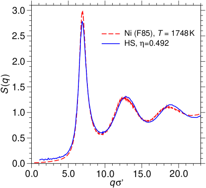
Figure 1: Static structure factor $S(q)$ of the hard sphere system and the Ni melt at coexistence, i.e. at the volume packing fraction $\eta=0.492$ for the hard spheres and at the temperature $T=1748$ K for Ni.

In order to study the structural differences between the bulk hard sphere fluid and the bulk Ni melt at coexistence, Fig. 1 displays the static structure factor [31] for both systems,

$$S(q)=\frac{1}{N}\left\langle{\Big{|}}\sum_{k=1}^{N}\exp[i\vec{q}\cdot\vec{r}_{k}]{\Big{|}}^{2}\right\rangle$$ (8)

with $\vec{r}_{k}$ the position of particle $k$ and $\vec{q}$ the three-dimensional wavevector (different from the two-dimensional wavevectors that we have considered in the previous section). To provide a better comparison between the structure factors for the two systems, we have multiplied the wave-number $q$ in Fig. 1 by $\sigma^{\prime}=\sigma$ for the hard sphere system and $\sigma^{\prime}=2.24$ Å for Ni (which is similar to the nearest neighbor distance, $r_{\rm NiNi}=2.42$ Å [37]).

Mainly two differences between the two systems can be inferred from Fig. 1. Towards $q\to 0$ the structure factor for Ni has a much lower amplitude, indicating that, at coexistence the Ni melt has a lower compressibility than the hard sphere system. Moreover, the amplitude of the first peak in $S(q)$ for Ni is slightly larger. But the overall shape of $S(q)$ is surprisingly similar for both systems which shows that the hard sphere system’s structure is very similar to that of Ni.

4.2 The structure of the solid-fluid interfaces

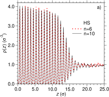
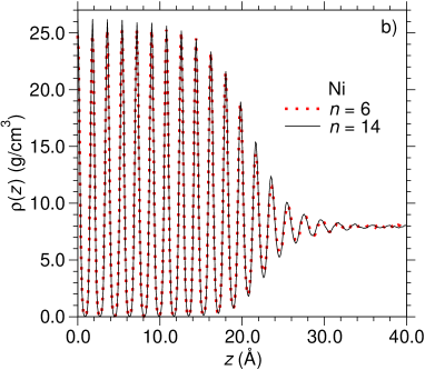
Figure 2: Density profiles for a) hard spheres and b) Ni. In each case, the profiles are shown for two different system sizes.

A simple quantity to characterize the structure of the interface is provided by the density profile $\rho(z)$ across the interface. To compute $\rho(z)$, the system is divided into slices of thickness $\Delta z$ and then, in each slice, one counts the number of particles and divides by the volume of the slice $L^{2}\Delta z$. The displacement of the lattice planes along the $z$-axis during the time evolution was corrected for each configuration. As for the order parameter profiles shown below, we have averaged the density profiles over the two interfaces in each system that are present due to periodic boundary conditions.

Figure 2 shows density profiles for the hard sphere system and Ni, in each case for two system sizes. The shape of the profiles is typical for inhomogeneous systems with crystal-fluid interfaces. In fact, very similar density profiles have been found for various systems with solid-liquid interfaces [13, 15, 16, 19, 20]. Whereas one observes huge oscillations in the crystalline region due to the presence of crystalline layers, in the fluid region $\rho(z)$ is constant. In between, i.e. in the interface region, the amplitude of the peaks decreases. Obviously, the size effects are very small for both considered systems. However, for the big systems the height of the peaks is slightly larger in the interface region. We note that although the density profiles have a very different shape in the solid and the liquid regions, both for the HS system and for Ni the differences in the average densities of the solid and the liquid phase are rather small. In the HS case, the solid density is about 10% higher ($\rho_{\rm s}=1.04$, $\rho_{\rm l}=0.9385$) and for Ni, it is about 5% higher ($\rho_{\rm s}=8.357$ g/cm³, $\rho_{\rm l}=7.928$ g/cm³). Due to this small difference between $\rho_{\rm l}$ and $\rho_{\rm s}$ the density is not a good order parameter for the investigation of interfacial properties such as the interfacial width.

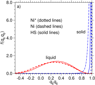
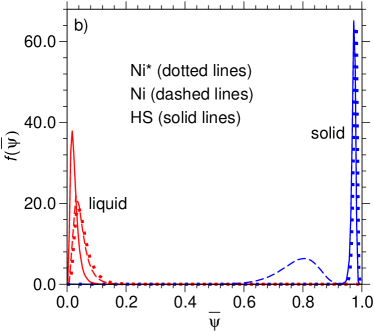
Figure 3: Probability distributions of the order parameter in Ni (broken lines) and the hard sphere system (solid lines) for the liquid and the fcc phase, as indicated; a) $q_{6}q_{6}$, b) $\bar{\Psi}$. Different time intervals for obtaining the average particle positions are considered for Ni; thereby, the dashed lines correspond to an interval of 0.1 ps and the dotted lines to 1 ps (the latter case is referred to as $Ni^{*}$).

Another possibility to characterize the structure of interfaces is provided by profiles of local order parameters. Steinhardt et al. [52] have proposed rotational-invariant order parameters in terms of expansions into spherical harmonics $Y_{lm}$,

$$Q_{l}(i)=\left(\frac{4\pi}{2l+1}\sum_{m=-l}^{l}{|\bar{Q}_{lm}|^{2}}\right)^{1/2}$$ (9)

with

$$\bar{Q}_{lm}(i)=\frac{1}{Z_{i}}\sum_{j=1}^{Z_{i}}{Y_{lm}(\theta(\vec{r}_{ij}),\phi(\vec{r}_{ij}))}\,,$$ (10)

where $\vec{r}_{ij}$ is the distance vector between a pair of neighboring particles $i$ and $j$, $Z_{i}$ is the number of neighbors within a given cut-off radius, and $\theta(\vec{r}_{ij})$ and $\phi(\vec{r}_{ij})$ are the polar bond angles with respect to an arbitrary reference frame.

Similar local order parameters have been introduced by ten Wolde et al. [53], defined by

$$q_{l}q_{l}(i)=\frac{1}{Z_{i}}\sum_{j=1}^{Z_{i}}{{\bf q}_{l}(i)\cdot{\bf q}_{l}(j)}\,.$$ (11)

The internal product in this sum is given by

$${\bf q}_{l}(i)\cdot{\bf q}_{l}(j)=\sum_{m=-l}^{l}{\tilde{q}_{lm}(i)\tilde{q}_{lm}(j)^{*}}$$ (12)

with

$$\tilde{q}_{lm}(i)=\frac{\bar{Q}_{lm}(i)}{\left(\sum_{m=-l}^{l}{|\bar{Q}_{lm}(i)|^{2}}\right)^{1/2}}\,.$$ (13)

In the following, we use the parameter $q_{6}q_{6}$ that is defined by Eqs. (11)-(13), setting $l=6$.

Another local order parameter used in this work was introduced by Morris [54]

$$\Psi(i)={\Big{|}}\frac{1}{N_{q}}\frac{1}{Z_{i}}\sum_{j=1}^{Z_{i}}\sum_{k=1}^{N_{q}}\exp(i\vec{q}_{k}\cdot\vec{r}_{ij}){\Big{|}}^{2}$$ (14)

where the wavevectors $\vec{q}_{k}$ are chosen such that in a perfect crystal

$$|\exp(i\vec{q}_{k}\cdot\vec{r}_{ij})|=1\,.$$ (15)

Again, $\vec{r}_{ij}$ is the distance vector between neighboring particles. With respect to the basis vectors of the fcc lattice with lattice constant $a$, $\vec{a}_{1}=a/2(1,1,0)$, $\vec{a}_{2}=a/2(0,1,1)$ and $\vec{a}_{3}=a/2(1,0,1)$, an appropriate choice of wavevectors is $\vec{b}_{1}=2\pi/a(-1,1,-1)$, $\vec{b}_{2}=2\pi/a(1,-1,1)$ and $\vec{b}_{3}=2\pi/a(1,1,-1)$. An additional average of $\Psi(i)$ over a particle with index $i$ and its neighboring particles yields

$$\bar{\Psi}(i)=\frac{1}{Z_{i}+1}\left(\Psi(i)+\sum_{j=1}^{Z_{i}}\Psi(j)\right)\;.$$ (16)

The parameter $\bar{\Psi}$ together with $q_{6}q_{6}$ is used in the following to distinguish solid particles from fluid particles and to identify the interfacial regions. To select the nearest neighbors we introduced the cut-off radii that correspond to the first minimum of the radial distribution function of the bulk liquid phase at coexistence.

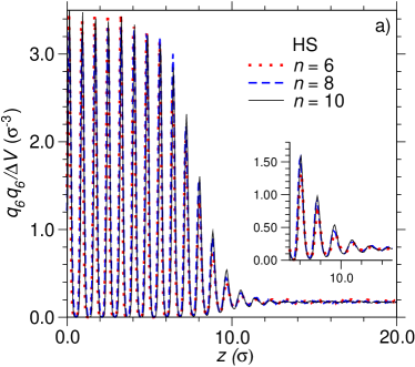
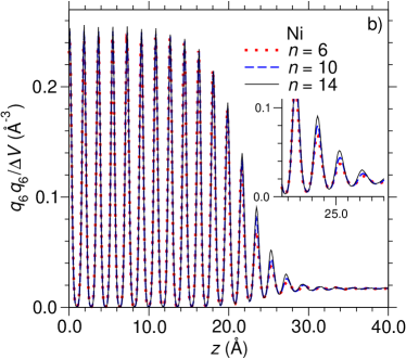
Figure 4: Profile for the order parameter $q_{6}q_{6}$, a) for hard spheres and b) for Ni. The inserts provide a magnification of the interface region.

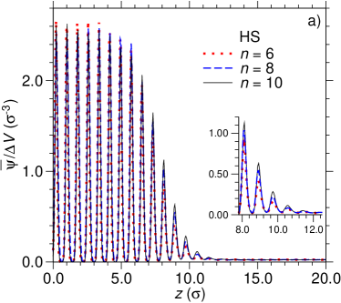
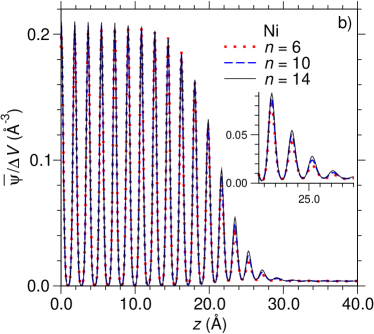
Figure 5: Profile for the order parameter $\bar{\Psi}_{r}$, a) for hard spheres and b) for Ni. The inserts provide a magnification of the interface region.

Figure 3 displays local order parameter distributions for the pure liquid and the pure solid phases. The distributions indicate that the considered order parameters are well-suited to distinguish liquid from solid particles. For the calculation of the local order parameters, we used time-averaged particle positions. To this end, for the hard sphere system, positions were averaged over 50 MC cycles. For Ni, the phonon’s degrees of freedom lead to a significant shift of the order parameter distributions. Using a time interval of 0.1 ps for the averaging of the particle positions in Ni, compared to an ideal fcc crystal the order parameter distributions for the crystal phase are broader and tend to shift to smaller values of the order parameter (see Fig. 3). For a time average over 1 ps the order parameter distributions are very similar to those for the hard spheres. However, since in Ni at $T_{\rm m}$ a time scale of 1 ps is already close to the time scale of particle diffusion in the melt, we have used a time averaging over 0.1 ps for the analysis of the interfacial properties that are presented in the following.

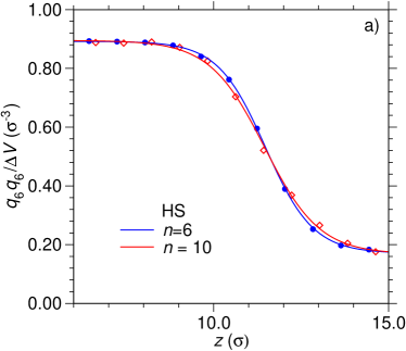
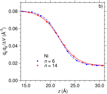
Figure 6: Coarse grained order parameter profile for $q_{6}q_{6}$ at the indicated system sizes, a) for hard spheres and b) for Ni. The solid lines are fits to a hyperbolic tangent function (Eq.6), see text.

In Figs. 4 and 5, profiles of the local order parameters are shown, i.e. the sum of the order parameter of the particles contained within a slice transversal to the solid-liquid interface divided by the volume of the slice $\Delta V=L^{2}\Delta z$. The profiles are calculated with a resolution (bin size) of 0.02 $\sigma$ for the hard spheres and 0.1 Å for Ni. The order parameter profiles show similar features as the density profiles. However, finite-size effects seem to be revealed in a more pronounced manner. Clearly, the height of the peaks in the interface region slightly increases with increasing system size.

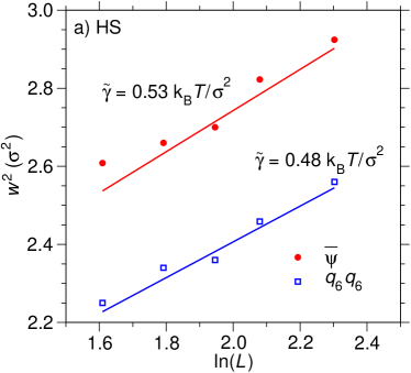
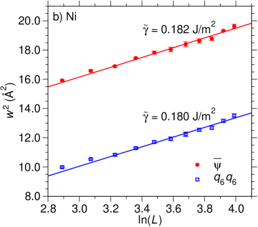
Figure 7: Mean-squared width $w^{2}$ as a function of $\ln L$, a) for hard spheres and b) for Ni. The values for $\tilde{\gamma}$ are obtained from the fits (solid lines).

To compute coarse-grained profiles we identify the minima in the fine-grid profiles of Figs. 4 and 5. These minima define the borders of nonuniform bins that match the crystalline layers. Then, we compute the average value of the order parameter in each of the latter bins. Examples for the resulting coarse-grained order parameter profiles for the case of $q_{6}q_{6}$ are displayed in Fig. 6. Here, the solid lines are fits with a hyperbolic tangent function, $\phi(z)=A-B\tanh[(z-z_{0})/w]$ (where $A$ and $B$ are parameters related to the bulk values of the order parameter, and $z_{0}$ and $w$ are the interface position and its effective width, respectively). Both for the hard spheres and Ni, the latter fits indicate that the width $w$ is larger for the big systems, as expected from CWT.

4.3 Estimate of the interfacial stiffness

In Fig. 7, the mean-squared width $w^{2}$, as obtained from the fits to the coarse-grained profiles for $q_{6}q_{6}$ and $\bar{\Psi}$, is plotted as a function of $\ln L$. The plot confirms the logarithmic increase of $w^{2}$ with the lateral system size, as predicted by CWT.

From the fits with Eq. (7), we estimate for the (100) orientation $\tilde{\gamma}=0.50\pm 0.05\,k_{B}T/\sigma^{2}$ for the hard-sphere system and $\tilde{\gamma}=0.18\pm 0.01$ J/m² for Ni. These values roughly agree with previous estimates, obtained by other methods. For hard spheres, Davidchack and Laird [14] found $\tilde{\gamma}=0.57\,k_{B}T/\sigma^{2}$ using a thermodynamic integration approach, while Mu et al. [55] obtained $\tilde{\gamma}\simeq 0.62\,k_{B}T/\sigma^{2}$ from the analysis of the capillary wave spectrum. However, Davidchack et al. [56] later criticized their result as being biased and rather suggested $\tilde{\gamma}=0.56\pm 0.02\,k_{B}T/\sigma^{2}$ when averaged over all interface orientations. For the (100) orientation, they suggest $\tilde{\gamma}\simeq 0.44\pm 0.03\,k_{B}T/\sigma^{2}$. However, their actual data reveal huge fluctuations, and the judgement of the actual accuracy may need reanalysis. For Ni, Hoyt et al. [17] determined the interfacial stiffness for the (100) orientation (and other orientations of the Ni fcc phase). Using a different EAM model and the analysis of the capillary wave spectrum to measure $\tilde{\gamma}$, they obtained $\tilde{\gamma}\approx 0.23$ J/m², which is slightly larger than our result.

5 Summary and Outlook

In this paper, we have presented a comparative study of melt-crystal interfaces for hard spheres and an embedded atom model for nickel. These rather diverse systems have been studied in analogous geometries, namely $L\times L\times L_{z}$ rectangular simulation boxes with periodic boundary conditions, at conditions where a crystalline slab, separated by two $L\times L$ interfaces oriented perpendicular to the $z$-direction, coexists with the fluid phase. The motivation for this study was to provide a better understanding of the information that one can extract from the simulation study of such interfaces, paying particular attention to finite size effects, and to limitations of the accuracy which are inherently due to the simulation setup. In fact, due to the translational invariance of the simulation geometry as a whole, the center of mass of the crystalline part is not fixed in space, but may fluctuate and diffuse along the $z$-axis. In addition, at phase coexistence in a finite box, fluctuations may occur when the size of the crystal (volume fraction of the box that is crystallized) changes. As a consequence, in each configuration that is analyzed one must locate the precise position along the $z$-axis where the lattice planes are (this was done via a fine-grid coarse graining) and then the time averages are found in such a way that the positions of lattice planes and interface centers coincide. It is clear that this is a delicate procedure and hence there is the need to watch out for possible systematic errors, which are not necessarily equally important for different kinds of systems, and for different simulation methods (e.g. MC and MD). In view of these caveats, it is gratifying to state that with the methods described in this paper, these problems seem reasonably well under control. Indeed, we find that the main difficulty in the interpretation of our results for the interfacial profiles and their width is the broadening by the capillary waves. This phenomenon, though well-known for vapor-liquid interfaces, has found comparatively little attention for the melt-crystal interface. Our results imply that the capillary wave broadening (for rough, non-facetted crystal surfaces) is present and important: while it makes a naive direct comparison with DFT calculations of interfacial profiles obsolete, it yields a relatively straightforward method for extracting the interfacial stiffness and the accuracy of this method seems to be competitive to other approaches.

As a next step we plan a detailed comparison with the alternative method where the Fourier spectrum of interfacial fluctuations is analyzed. For vapor-liquid type systems, such comparisons can be found in the literature, but for the melt-crystal interface a comprehensive comparative assessment of different methods still is lacking. Of course, for applications in crystal nucleation and growth phenomena very accurate estimates for the interfacial stiffness are indispensable.

Acknowledgments: We thank Lorenz Ratke for a critical reading of the manuscript. We are grateful to the German Science Foundation (DFG) for financial support in the framework of the SPP 1296. We acknowledge a substantial grant of computer time at the Jülich multiprocessor system (JUMP) of the John von Neumann Institute for Computing (NIC) and at the ZDV of the University of Mainz.

References

References

- [1] W. D. Kaplan and Y. Kauffmann, Ann. Rev. Mater. Res. 36, 1 (2006).
- [2] U. Gasser, E. R. Weeks, A. Schofield, P. N. Pusey, and D. A. Weitz, Science 292, 258 (2001).
- [3] R. P. A. Dullens, D. G. A. L. Aarts, and W. K. Kegel, Phys. Rev. Lett. 97, 228301 (2006).
- [4] V. Prasad, D. Semwogerere, and E. R. Weeks, J. Phys.: Condens. Matter 19, 113102 (2007).
- [5] J. Hernández-Guzmán and E. R. Weeks, preprint arXiv:0808.1576v.
- [6] H. Emmerich, Adv. Phys. 57, 1 (2008).
- [7] K. R. Elder, M. Katakowski, M. Haataja, and M. Grant, Phys. Rev. Lett. 88, 245701 (2002).
- [8] S. van Teeffelen, R. Backofen, A. Voigt, and H. Löwen, preprint arXiv:0902.3363v1.
- [9] A. J. Archer and R. Evans, J. Chem. Phys. 121, 4246 (2004).
- [10] S. van Teeffelen, C. N. Likos, and H. Löwen, Phys. Rev. Lett. 100, 108302 (2008).
- [11] D. W. Oxtoby, in Liquids, Freezing and the Glass Transition, Les Houches, Session Ll, 1989, eds. J.-P. Hansen, D. Levesque, and J. Zinn-Justin, (North-Holland, Amsterdam, 1991), p. 147; H. Löwen, Phys. Rep. 237, 249 (1994).
- [12] F. P. Buff, R. A. Lovett, and F. H. Stillinger, Phys. Rev. Lett. 15, 621 (1965); J. D. Weeks, J. Chem. Phys. 67, 3106 (1977); D. Bedeaux and J. D. Weeks, J. Chem. Phys. 82, 972 (1985).
- [13] R. L. Davidchack and B. B. Laird, J. Chem. Phys. 108, 9452 (1998).
- [14] R. L. Davidchack and B. B. Laird, Phys. Rev. Lett. 85, 4751 (2000).
- [15] H. E. A. Huitema, M.J. Vlot, and J.P. van der Eerden, J. Chem. Phys. 111, 4714 (1999).
- [16] J. Jesson and P. A. Madden, J. Chem. Phys. 113, 5935 (2000).
- [17] J. J. Hoyt, M. Asta, and A. Karma, Phys. Rev. Lett. 86, 5530 (2001).
- [18] M. Asta, J. J. Hoyt, and A. Karma, Phys. Rev. B 66, 1000101 (2002).
- [19] A. Kerrache, J. Horbach, and K. Binder, EPL 81, 58001 (2008).
- [20] D. Buta, M. Asta, and J. J. Hoyt, Phys. Rev. E 78, 031605 (2008).
- [21] D. Frenkel, Physica A 263, 26 (1999).
- [22] J. E. Kirkwood, Phase Transformations in Solids (Wiley, New York, 1951).
- [23] B. J. Alder and T. E. Wainwright, J. Chem. Phys. 27, 1208 (1957).
- [24] W. W. Wood and J. D. Jacobson, J. Chem. Phys. 27, 1207 (1957).
- [25] W. G. Hoover and F. H. Ree, J. Chem. Phys. 49, 3609 (1968).
- [26] D. P. Landau and K. Binder, A Guide to Monte Carlo Simulations in Statistical Physics (Cambridge University Press, Cambridge, 2000).
- [27] D. Frenkel and B. Smit, Understanding Molecular Dynamics (Academic, London, 2002).
- [28] W. Krauth, Statistical Mechanics: Algorithms and Computations (Oxford University Press, Oxford, 2006).
- [29] N. F. Carnahan and K.E.Starling, J. Chem. Phys. 51, 635 (1969).
- [30] K. R. Hall, J. Chem. Phys. 57, 2252 (1972).
- [31] J.-P. Hansen and I. R. McDonald, Theory of Simple Liquids (Academic, San Diego, 1986).
- [32] E. G. Noya and E. de Miguel, J. Chem. Phys. 128, 154507 (2008).
- [33] N. B. Wilding and A. D. Bruce, Phys. Rev. Lett. 85, 5138 (2000).
- [34] A. Fortini and M. Dijkstra, J. Phys.: Condens. Matter 18, L371 (2006).
- [35] T. Zykova-Timan, J. Horbach, and K. Binder, to be submitted.
- [36] S. M. Foiles, Phys. Rev. B 32, 3409 (1985).
- [37] R. E. Rozas, J. Horbach, J. Brillo, and J. Schmitz, to be submitted.
- [38] M. P. Allen and D. J. Tildesley, Computer simulations of Liquids (Clarendon, Oxford, 1987).
- [39] T. B. Massalski, Binary Alloy Phase Diagrams (American Society for Metals, Ohio, 1986).
- [40] H. C. Andersen, J. Chem. Phys. 72, 2384 (1980).
- [41] F. Schmid and K. Binder, Phys. Rev. B 46, 13553 (1992).
- [42] M. Hasenbusch and K. Pinn, Physica A 192, 342 (1992).
- [43] M. Müller and G. Münster, J. Stat. Phys. 118, 669 (2005).
- [44] A. Werner, F. Schmid, M. Müller, and K. Binder, J. Chem. Phys. 107, 8175 (1997).
- [45] A. Werner, F. Schmid, M. Müller, and K. Binder, Phys. Rev. E 59, 728 (1999).
- [46] A. Werner, M. Müller, F. Schmid, and K. Binder, J. Chem. Phys. 110, 1221 (1999).
- [47] R. L. C. Vink and J. Horbach, J. Phys.: Condens. Matter 16, S3807 (2004).
- [48] R. L. C. Vink, J. Horbach, and K. Binder, J. Chem. Phys. 122, 134905 (2005).
- [49] D. Jasnow, Rep. Progs. Phys. 47, 1059 (1984).
- [50] T. Kerle, J. Klein, and K. Binder, Eur. Phys. J. B 7, 401 (1999).
- [51] K. Binder and M. Müller, Int. J. Mod. Phys. C 11, 1093 (2000).
- [52] P. J. Steinhardt, D. R. Nelson, and M. Ronchetti, Phys. Rev. B 28, 784 (1983).
- [53] P. R. ten Wolde, M. J. Ruiz-Montero, and D. Frenkel, Phys. Rev. Lett. 75, 2714 (1995).
- [54] J. R. Morris, Phys. Rev. B 66, 144104 (2002).
- [55] Y. Mu, A. Houk, and X. Song, J. Phys. Chem. B 109, 6500 (2005).
- [56] R. L. Davidchack, J. R. Morris, and B. B. Laird, J. Chem. Phys. 125, 094710 (2006).