Stratification in the Preferential Attachment Network

Abstract

We study structural properties of trees grown by preferential attachment. In this mechanism, nodes are added sequentially and attached to existing nodes at a rate that is strictly proportional to the degree. We classify nodes by their depth $n$, defined as the distance from the root of the tree, and find that the network is strongly stratified. Most notably, the distribution $f_{k}^{(n)}$ of nodes with degree $k$ at depth $n$ has a power-law tail, $f_{k}^{(n)}\sim k^{-\gamma(n)}$. The exponent grows linearly with depth, $\gamma(n)=2+\frac{n-1}{\langle n-1\rangle}$, where the brackets denote an average over all nodes. Therefore, nodes that are closer to the root are better connected, and moreover, the degree distribution strongly varies with depth. Similarly, the in-component size distribution has a power-law tail and the characteristic exponent grows linearly with depth. Qualitatively, these behaviors extend to a class of networks that grow by a redirection mechanism.

I Introduction

Unlike the ordered crystalline structure of solid-state matter ck , a wide array of natural and man-made networks ranging from chemical reaction pathways and social groups to the Internet and airline routes have a strongly heterogeneous structure ws ; ab ; dm . The connectivity of an element in such complex networks varies across multiple scales: most of the nodes have a very small number of connections, but there is also a small number of highly connected hubs.

The degree distribution measures the connectivity in the network and is widely used to characterize the structure of complex networks. This distribution uniformly samples all nodes in the network. Yet, given the highly heterogeneous structure of complex networks, it is plausible that different subsets of nodes have very different structural characteristics. In this study, we show that the degree distribution strongly varies in a given network.

We focus on the basic preferential attachment mechanism has ; ba which provides a useful model of growing networks krl ; dms . The preferential attachment network, where nodes are added sequentially and attached to existing nodes at a rate proportional to the degree, demonstrates how a “rich-gets-richer” mechanism generates networks with highly connected nodes and with a broad distribution of connectivities.

For the preferential attachment network, which has a tree topology, it is natural kr01 ; kcmdsh to classify nodes by their depth $n$, defined as the distance from the root. This depth representation divides the network into layers: the first layer includes nodes with depth $n=1$, the second layer includes nodes with depth $n=2$, etc. Our main result is that the distribution $f_{k}^{(n)}$ of nodes with degree $k$ at the $n$th layer has an algebraic tail with a depth-dependent exponent,

$$f_{k}^{(n)}\sim k^{-\gamma(n)},\qquad\gamma(n)=2+\frac{n-1}{\langle n-1\rangle}.$$ (1)

Interestingly, the exponent $\gamma$ grows linearly with depth, and thus, nodes that are closer to the root tend to be better connected. The degree distribution (1) matches the total degree distribution, $f_{k}^{\rm total}\sim k^{-3}$, only at the average depth, $n=\langle n\rangle$. The tail of the degree distribution is overpopulated with respect to the total distribution below the average depth and conversely, the tail is underpopulated above the average depth. Therefore, the network is stratified. In particular, the structure of the network changes with the depth because the degree distribution is not uniform across the network.

This qualitative behavior extends to other structural features of the network. In particular, the in-component size distribution that measures the total number of nodes that emanate from a given node has a very similar behavior as in any layer the distribution has an algebraic tail and the corresponding exponent grows linearly with depth. Furthermore, the tail of the in-component size distribution is shallow below the average depth but steep above the average depth. We generalize these results to the broader class of redirection networks, and find similar network structures.

The rest of this paper is organized as follows. We describe the preferential attachment network and discuss the distribution of depth in section II. We analyze the depth dependence of the degree distribution and the in-component size distribution in sections III and IV, respectively. We briefly discuss redirection networks in section V and conclude in section VI. The correction to the leading asymptotic behavior in large but finite networks is derived in Appendix A.

II The Preferential Attachment Network

In the preferential attachment model of network growth, nodes are added one at a time. Each new node is linked to a target node that is selected with probability that is strictly proportional to the degree. This attachment mechanism favors strongly connected nodes over weakly connected ones. We assume that initially there is a single node, the root. Since each attachment event adds one node and one link, the network maintains a tree topology.

Figure 1: Illustration of the redirection process. The new node, indicated by a bullet, links with equal probabilities to a randomly selected node or to its parent.

We use link redirection kr01 to emulate preferential attachment. In the redirection process, following the addition of a new node, an existing node is selected at random. With probability $\frac{1}{2}$, the new node links to this randomly selected node, and with equal probability $\frac{1}{2}$, the new node links to the parent of the selected node, as in figure 1. A node with degree $k$ has one outgoing link and $k-1$ incoming links, and the total probability $P_{k}$ of attachment to such a node includes two contributions: the probability of a direct link is $\frac{1}{2N}$ where $N$ is the total number of nodes while the probability of a redirected link is $\frac{k-1}{2N}$. Thus, the total attachment probability $P_{k}=\frac{k}{2N}$ is strictly proportional to the degree, and this link redirection process is equivalent to preferential attachment. Redirection does not explicitly involve the degree of a node, and is therefore convenient for both theoretical analysis and numerical simulation kr01 ; kr02 .

Let us label the nodes in the network by their depth $n$, defined as the distance from the root. With this definition, nodes are grouped by layers: the first layer consists of nodes with $n=1$, the second layer consists of nodes with $n=2$, etc, as illustrated in figure 2. As a preliminary step, we evaluate $M_{n}(N)$, the expected number of nodes at the $n$th layer in a network with $N$ nodes. This quantity obeys the difference equation

$$M_{n}(N+1)-M_{n}(N)=\frac{M_{n-1}(N)+M_{n}(N)}{2N}.$$ (2)

The boundary condition is $M_{0}=1$ because there is a single root. The first gain term on the right hand side accounts for direct links and the second term for redirected links. Also, the right hand side is inversely proportional to the total number of nodes. This difference equation can be converted into a differential equation when the network is large, $N\gg 1$,

$$\frac{dM_{n}}{dN}=\frac{M_{n-1}+M_{n}}{2N}.$$ (3)

Henceforth, the $N$-dependence is implicit. The number of nodes at the first layer, $M_{1}\sim N^{1/2}$, follows from $dM_{1}/dN=M_{1}/(2N)$ kr01 . In general, the transformation $M_{n}=M_{1}m_{n}$ reduces equation (3) to $dm_{n}/dN=m_{n-1}/(2N)$ with the boundary condition $m_{1}=1$. Solving this latter equation recursively yields $m_{2}=\frac{1}{2}\ln N$, $m_{3}=\frac{1}{2!}\left(\frac{1}{2}\ln N\right)^{2}$, and in general, $m_{n}=\frac{1}{(n-1)!}\left(\frac{1}{2}\ln N\right)^{n-1}$. Therefore, the distribution of depth is

$$M_{n}\sim N^{1/2}\frac{\left(\frac{1}{2}\ln N\right)^{n-1}}{(n-1)!}.$$ (4)

Accordingly, the distribution of the variable $n-1$ is Poissonian and is fully characterized by the average that grows logarithmically with the total number of nodes,

$$\langle n-1\rangle\simeq\frac{1}{2}\ln N.$$ (5)

Furthermore, the variance, $\sigma^{2}=\langle(n-1)^{2}\rangle-\langle n-1\rangle^{2}$, equals the average, $\sigma^{2}\simeq\frac{1}{2}\ln N$.

Figure 2: Illustration of the layer structure. Indicated in the figure are the first three layers.

In principle, the Poisson depth distribution (4) is Gaussian in the vicinity of the average depth. Specifically, the the variable $\xi=[(n-1)-\langle n-1\rangle]/\sigma$ obeys Gaussian statistics. In practice, since the depth and the variance both grow logarithmically with the network size, statistics of the depth are not fully captured by the Gaussian distribution even in very large networks.

We measure the depth in units of the average using the normalized depth

$$y=\frac{n-1}{\langle n-1\rangle}.$$ (6)

The average number of nodes with normalized depth $y$ grows as a power-law with the total number of nodes,

$$M_{n}\sim N^{\nu},\qquad\nu=\frac{1+y-y\ln y}{2}.$$ (7)

This result is obtained by substituting $n-1=\frac{y}{2}\ln N$ into (4) and then evaluating the quantity $\ln M_{n}\simeq\nu\ln N$ using the Stirling formula, $\ln n!\sim n\ln n-n$. As expected, the total number of nodes at the average depth is proportional to the system size, $\nu(1)=1$, and the total number of nodes at the first layer is consistent with (4), $\nu(0)=\frac{1}{2}$. In general, the exponent $\nu$ that characterizes the population of nodes at a given depth is continuously varying, and in particular, this exponent vanishes at a nontrivial maximal depth, $y_{\rm max}=3.59112$, specified as the root of the equation $1+y_{\rm max}=y_{\rm max}\ln y_{\rm max}$. Therefore, there are no nodes with depth larger than this maximal depth, $0\leq y\leq y_{\rm max}$.

III The Degree Distribution

We now discuss the unnormalized degree distribution, $F_{k}^{(n)}$, defined as the average number of nodes with depth $n$ and degree $k$. We begin with the first layer, $n=1$, where the quantity $F_{k}^{(1)}$ obeys the rate equation

$$\frac{dF_{k}^{(1)}}{dN}=\frac{(k-1)F_{k-1}^{(1)}-kF_{k}^{(1)}}{2N}+\frac{M_{0}+M_{1}}{2N}\,\delta_{k,1}.$$ (8)

Throughout this study, we assume that the network is large and treat $N$ as a continuous variable. In other words, we use rate equations as in (3) rather than difference equations as in (2). The first two gain terms on the right hand side account for augmentation in the degree of an existing node due to attachment, and the corresponding rate of attachment to nodes with degree $k$ equals the attachment probability $P_{k}=\frac{k}{2N}$. The last two gain terms, accounting respectively for redirected links and direct links, correspond to the new nodes.

We now introduce the degree distribution $f_{k}^{(1)}$, the fraction first layer nodes with degree $k$, defined by

$$F_{k}^{(1)}=M_{1}f_{k}^{(1)}.$$ (9)

This distribution is normalized, $\sum_{k}f_{k}^{(1)}=1$. With the definition (9), the evolution equation (8) becomes

$$\frac{M_{0}+M_{1}}{2N}f_{k}^{(1)}=M_{1}\frac{(k-1)f_{k-1}^{(1)}-kf_{k}^{(1)}}{2N}+\frac{M_{0}+M_{1}}{2N}\,\delta_{k,1}.$$

In writing this equation, we kept the rate of change of the total number of nodes in the first layer $dM_{1}/dN$ given by (3), but neglected the sub-dominant $N$-dependence of the normalized degree distribution $df_{k}^{(1)}/dN$. The number of nodes at the zeroth layer, $M_{0}=1$, is negligible compared with the number of nodes at the first layer, $M_{0}\ll M_{1}$, and as a result, the degree distribution $f_{k}^{(1)}$ obeys the simple recursion equation

$$(k+1)f_{k}^{(1)}=(k-1)f_{k-1}^{(1)}+\delta_{k,1}.$$ (10)

Hence, the degree distribution is $f_{k}^{(1)}=\frac{1}{1\cdot 2},\frac{1}{2\cdot 3},\frac{1}{3\cdot 4}$ for $k=1,2,3$, and in general, this quantity is remarkably simple,

$$f_{k}^{(1)}=\frac{1}{k(k+1)}.$$ (11)

This distribution is properly normalized, $\sum_{k}f_{k}^{(1)}=1$. Interestingly, the tail of the normalized degree distribution, $f_{k}^{(1)}\sim k^{-2}$ is overpopulated with respect to that of the total degree distribution, $f_{k}^{\rm total}\sim k^{-3}$ ba ; krl ; dms . Nevertheless, the expected number of nodes with degree $k$ at the first layer, $F_{k}^{(1)}\sim N^{1/2}k^{-2}$, remains smaller than the total number of nodes with degree $k$, $F_{k}^{\rm tot}\sim Nk^{-3}$, because the maximal degree in the network is bounded, $k\ll N^{1/2}$. The maximal degree in the network, $k_{\rm max}\sim N^{1/2}$, is estimated by equating the cumulative degree distribution $Q_{k}=\sum_{j\geq k}F^{\rm tot}_{j}\sim Nk^{-2}$ to one, $Q_{k}\sim 1$. Equation (11) clearly shows that nodes at the first layer tend to be much more connected compared with the rest of the network.

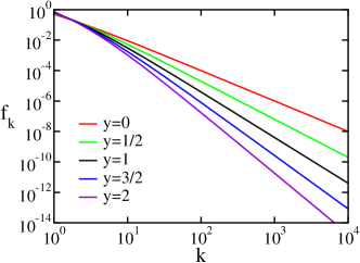
Figure 3: The degree distribution at different depths. Shown is the closed form expression (14) for five, equally-spaced, values of the normalized depth $y$ defined in (6).

The equation governing $F_{k}^{(n)}$, the average number of nodes with degree $k$ at the $n$th layer, is given by a straightforward generalization of (8),

$$\frac{dF_{k}^{(n)}}{dN}=\frac{(k-1)F_{k-1}^{(n)}-kF_{k}^{(n)}}{2N}+\frac{M_{n-1}+M_{n}}{2N}\,\delta_{k,1}.$$ (12)

Following the steps leading to (10), the degree distribution, $f_{k}^{(n)}$, defined as in (9), $F_{k}^{(n)}=M_{n}f_{k}^{(n)}$, obeys the recursion equation

$$(k+1+y)f_{k}^{(n)}=(k-1)f_{k-1}^{(n)}+(1+y)\delta_{k,1}$$ (13)

with the shorthand notation $y=M_{n-1}/M_{n}$. The parameter $y$ is equivalent to the normalized depth defined in (6). The degree distribution follows immediately from the recursion equation (13). First, the fraction of leafs is $f_{1}^{(n)}=(1+y)(2+y)$. Second, using the ratio $f_{k}^{(n)}/f_{k-1}^{(n)}=(k-1)(k+1+y)$ and the following property of the Gamma function, $\Gamma(x+1)/\Gamma(x)=x$, we express the degree distribution in a closed form in terms of the Gamma function,

$$f_{k}^{(n)}=(1+y)\frac{\Gamma(2+y)\Gamma(k)}{\Gamma(k+2+y)}.$$ (14)

Therefore, there is a family of degree distributions, parameterized by the normalized depth $y$. From the well-known asymptotic behavior of the ratio of Gamma functions, $\lim_{x\to\infty}[x^{a}\Gamma(x)/\Gamma(x+a)]=1$, we find that the degree distribution has a power-law tail,

$$f_{k}^{(n)}\simeq A\,k^{-\gamma(n)}$$ (15)

for $k\gg 1$. The characteristic exponent $\gamma=2+y$ grows linearly with depth

$$\gamma(n)=2+\frac{n-1}{\langle n-1\rangle},$$ (16)

and the prefactor is $A=(1+y)\,\Gamma(2+y)$. The power-law behavior (15) strictly holds only for infinitely large networks. The appendix describes the correction to this leading asymptotic behavior in large but finite networks.

As shown in figure 3, the degree distribution is not uniform across the network and the characteristic exponent $\gamma(n)$ increases linearly with depth $n$. Therefore, nodes that are closer to the root tend to have a larger number of connections. The tail of the degree distribution is overpopulated with respect to the total degree distribution below the average depth as $\gamma<3$ for $n<\langle n\rangle$. Similarly, the tail is underpopulated with respect to the total degree distribution above the average depth, $\gamma>3$ for $n>\langle n\rangle$. The degree distribution at the average depth equals the total degree distribution $f_{k}^{(\langle n\rangle)}=f_{k}^{\rm total}=4/[k(k+1)(k+2)]$ because the depth distribution (4) gradually narrows around the average depth (5) as the network grows. Nevertheless, there is still an appreciable number of nodes at depths other than the average, as indicated by the power-law growth in (7). Finally, we note that since the depth is bounded by the maximum value $y_{\rm max}=3.59112$, the characteristic exponent has a nontrivial upper bound, $2\leq\gamma\leq 5.59112$.

IV The in-component size distribution

Each node is in itself a root of the sub-tree that emanates from it. This sub-tree is termed the in-component of the node and we denote by $s$ the size of the in-component. We note that the size of the in-component is at least as large as the degree of the node: $s\geq k$. The minimal size $s=1$ corresponds to dangling nodes without descendants. Let $G_{s}^{(n)}$ be the average number of $n$th layer nodes with in-components of size $s$. This quantity satisfies the rate equation

$$\frac{dG_{s}^{(n)}}{dN}=\frac{\left(s-\frac{3}{2}\right)G_{s-1}^{(n)}-\left(s-\frac{1}{2}\right)G_{s}^{(n)}}{N}+\frac{M_{n-1}+M_{n}}{2N}\delta_{s,1}.$$

With probability $\frac{s}{N}$ a node in an in-component of size $s$ is selected at random following the addition of a new node, and all such events, with the exception of redirection away from the root of the sub-tree, result in attachment of an additional node to the in-component. Since redirection away from the root of the sub-tree occurs with probability $\frac{1}{2N}$, the probability of attaching an additional node to the in-component equals $\frac{s-1/2}{N}$. Hence, the first two terms on the right hand side. The last two terms are as in (12).

The normalized distribution $g_{s}^{(n)}$ of nodes with in-degree $s$ and depth $n$, defined by $G_{s}^{(n)}=M_{n}\,g_{s}^{(n)}$, obeys the recursion equation

$$\left(s+\frac{y}{2}\right)g_{s}^{(n)}=\left(s-\frac{3}{2}\right)g_{s-1}^{(n)}+\frac{1+y}{2}\delta_{s,1}~{}.$$ (17)

This equation is very similar in structure to the equation (13) governing the degree distribution. Dangling nodes have $s=k=1$ and therefore, $g_{1}^{(n)}=f_{1}^{(n)}=(1+y)(2+y)$. Using the ratio $g_{s}^{(n)}/g_{s-1}^{(n)}=(y-3/2)/(s+y/2)$, we obtain the in-component size distribution in closed form

$$g_{s}^{(n)}=\frac{1+y}{2+y}\frac{\Gamma\left(2+\frac{y}{2}\right)}{\Gamma\left(\frac{1}{2}\right)}\frac{\Gamma\left(s-\frac{1}{2}\right)}{\Gamma\left(s+1+\frac{y}{2}\right)}~{}.$$ (18)

Again, there is a family of distributions that is governed by $y$. Therefore, the in-component size distribution has a power-law tail

$$G_{s}^{(n)}\simeq B\,s^{-\beta(n)}$$ (19)

and the characteristic exponent varies continuously with depth, $\beta=(3+y)/2$ or

$$\beta(n)=\frac{3}{2}+\frac{1}{2}\frac{n-1}{\langle n-1\rangle}.$$ (20)

The prefactor in (19) is $B=(1+y)\Gamma(1+y/2)/\sqrt{4\pi}$.

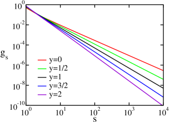
Figure 4: The in-component size distribution at different depths. Shown is the closed form expression (18) for $y=0,1/2,1,3/2,2$.

The in-component size distribution is very similar to the degree distribution (Figure 4). Nodes that are closer to the root tend to have larger in-components. The tail of the in-component size distribution is overpopulated below the average depth, $\beta<2$ when $n<\langle n\rangle$, while the tail is underpopulated above the average depth, $\beta>2$ for $n>\langle n\rangle$. The in-component size distribution matches the total distribution at the average depth, $G_{s}^{(\langle n\rangle)}=G_{s}^{{\rm total}}=2\,[4s^{2}-1]^{-1}$. Moreover, the in-component size distribution is steepest, $\beta_{\rm max}=4.29556$, at the maximal depth $y_{\rm max}=5.59112$.

For completeness, we also quote the in-component size distribution in the first layer,

$$g_{s}^{(1)}=\frac{1}{\sqrt{4\pi}}\frac{\Gamma\left(s-\frac{1}{2}\right)}{\Gamma(s+1)}~{},$$ (21)

and the corresponding tail, $g_{s}^{(1)}\sim s^{-3/2}$.

V Redirection networks

We briefly discuss the broader class of redirection networks kr01 . This family of networks is also grown by sequential addition of nodes. Subsequent to the addition of a new node, one existing node is selected at random. With the redirection probability $r$, the new node attaches to the parent of the randomly selected node while with the complementary probability $1-r$, the new nodes attaches to the randomly selected node itself. Redirection networks are therefore parameterized by the redirection probability $r$. The probability $P_{k}$ of attachment to a node of degree $k$ varies linearly with the degree, $P_{k}=(k-1)r+(1-r)$ or equivalently,

$$P_{k}=\frac{kr+1-2r}{N}.$$ (22)

As mentioned above, the special case $r=1/2$ yields the preferential attachment network. The limiting case $r=0$ corresponds to the random recursive tree where the attachment probability is uniform jmr ; bp ; ld ; pn ; hmm ; dek ; fsh .

The depth distribution obeys the following generalization of (3)

$$\frac{dM_{n}}{dN}=\frac{(1-r)M_{n-1}+rM_{n}}{N}.$$ (23)

Here, the first gain term accounts for direct links and the second term, for redirected links. The depth distribution is always Poissonian

$$M_{n}\sim N^{r}\frac{\left[(1-r)\ln N\right]^{n-1}}{(n-1)!}$$ (24)

and fully characterized by the average $\langle n-1\rangle\simeq(1-r)\ln N$.

The degree distribution is obtained by replacing the attachment probability $P_{k}=\frac{k}{2N}$ in (12) with (22). We skip the straightforward derivation of the degree distribution and merely quote the final result,

$$f_{k}^{(n)}=\frac{r+y-ry}{1+y-ry}\frac{\Gamma\left(\frac{1+r+y-ry}{r}\right)}{\Gamma\left(\frac{1-r}{r}\right)}\frac{\Gamma\left(k+\frac{1-2r}{r}\right)}{\Gamma\left(k+\frac{1+y-ry}{r}\right)}.$$ (25)

The parameter $y$ is the same normalized depth of (6) with the appropriate average $\langle n-1\rangle\simeq(1-r)\ln N$. Therefore, the degree distribution decays algebraically as in (15) with the exponent $\gamma=2+[(1-r)y]/r$ or equivalently

$$\gamma(n)=2+\frac{1-r}{r}\frac{n-1}{\langle n-1\rangle}.$$ (26)

The in-component size distribution

$$g_{s}^{(n)}=\frac{r+y-ry}{1+y-ry}\frac{\Gamma(2+y-ry)}{\Gamma(1-r)}\frac{\Gamma(s-r)}{\Gamma(s+1+y-ry)}$$ (27)

is obtained by replacing the attachment probability $\frac{s-1/2}{N}$ in (17) with $\frac{s-r}{N}$. As expected, this distribution decays algebraically as in (19) with the exponent

$$\beta(n)=1+r+(1-r)\frac{n-1}{\langle n-1\rangle}.$$ (28)

There is no substantive change in the behaviors of the degree distribution and the in-component size distribution. These distributions are characterized by power-law tails that become steeper with increasing depth, so that the further from the root a node is, the less likely that the node is highly connected. Generally, the degree distribution is non-uniform throughout the network.

VI conclusions

In conclusion, we studied how the degree distribution depends on depth, defined as the distance from the root, in the preferential attachment network and found that the network is strongly stratified. There is a family of degree distributions that is parameterized by the depth and the total degree distribution is a special case that corresponds to the behavior at the average depth. The degree distribution has a shallow power-law tail below the average depth and a steep tail above the average depth as the characteristic exponent grows linearly with depth. Interestingly, this exponent has a non-trivial upper bound. The in-component size distribution exhibits very similar qualitative behaviors.

The structure of the network changes considerably with the depth as nodes that are closer to the root tend to have a larger number of connections. Such stratification is empirically observed in complex networks including the internet chkss , and can be intuitively understood as follows. There are strong correlations between the depth of a node and its age because young nodes must be less connected. Since younger nodes are also further from the root, there are correlations between the degree and the depth. A natural complementary classification of the nodes is by their age, and we anticipate that similarly, the degree distribution exhibits age dependence.

The above results are not limited to trees. This is seen from a generalization of the preferential attachment process where new nodes attach to two nodes: one target node that is selected with probability proportional to its degree and one, randomly selected, parent of the target node. Thus, each new node adds a three-node cycle, and the network has at least as many cycles as there are nodes. Yet, the governing equations do not change and the behavior of the degree distribution and in-component size distribution are basically, the same bk .

One issue, open to further investigations, is the behavior in finite systems. The analysis in the appendix relies on on the continuum approximation. Yet, this approximation is asymptotically exact for degrees that are much smaller than the maximal one. A discrete approach with difference equations, rather than differential ones, is necessary kk ; dms2 ; kr02-a to determine the behavior for the degrees that are of the order of the maximal degree.

Appendix A Finite Networks

Throughout this investigation, we implicitly considered the leading asymptotic behavior for large networks. In particular, the sub-dominant dependence of the normalized degree distribution on the size of the network was ignored in (13). However, the logarithmic dependencies of the average depth and the variance suggest that extremely large networks may be needed to clearly observe the large-$N$ asymptotics (15).

To investigate how the degree distribution depends on the total number of nodes $N$, we rewrite the governing equation (12) in continuum form for large $k$,

$$\frac{\partial F}{\partial N}+\frac{1}{2N}\frac{\partial}{\partial k}\left(kF\right)=0.$$ (29)

In deriving this equation, we omitted the superscript and the subscript, $F\equiv F_{k}^{(n)}$. We now include the term $\partial f/\partial N$ describing how the degree distribution changes with system size in the evolution equation for the normalized distribution, defined by $F=Mf$,

$$2N\frac{\partial f}{\partial N}+k\frac{\partial f}{\partial k}+(2+y)f=0.$$ (30)

The normalized depth (6) is $y=2(n-1)/\ln N$ and therefore, $dy/dN=-y/\left(N\ln N\right)$. We now assume that the power-law tail (15) is modified by a correction, $f(k,N)\simeq A\,k^{-(2+y)}u(k,N)$. From (30), the correction function $u$ satisfies

$$\frac{\partial u}{\partial k}+2y\frac{\ln k}{k\ln N}u=0$$ (31)

Therefore, the correction function is log-normal, $u=\exp[-2y(\ln k)^{2}/\ln N]$, and the normalized distribution has the following tail

$$f_{k}^{(n)}\simeq A\,k^{-2-y}\,\exp\left[-2y\frac{(\ln k)^{2}}{\ln N}\right].$$ (32)

Indeed, the correction is irrelevant for infinitely large networks: $u\to 1$ when $N\to\infty$. For large but finite systems, there are two consequences. First, at moderate degrees, the correction is sub-dominant and the tail is power-law, although the exponent may appear slightly larger than the asymptotic value (16). Second, at large degrees, the correction is dominant and the tail is log-normal.

References

- (1) C. Kittel, Introduction to Solid State Physics, (Wiley, New York, 2004).
- (2) D. J. Watts and S. H. Strogatz, Nature 393, 440 (1998).
- (3) R. Albert and A. L. Barabasi, Rev. Mod. Phys. 74, 47 (2002).
- (4) S. N. Dorogovtsev and J. F. F. Mendes, Adv. in Phys. 51, 1079 (2002).
- (5) H. A. Simon, Biometrica 42, 425 (1955); Infor. Control 3, 80 (1960).
- (6) A. L. Barabasi and R. Albert, Science 286, 509 (1999).
- (7) P. L. Krapivsky, S. Redner, and F. Leyvraz, Phys. Rev. Lett. 85, 4629 (2000).
- (8) S. N. Dorogovtsev, J. F. F. Mendes, and A. N. Samukhin, Phys. Rev. Lett. 85, 4633 (2000).
- (9) P. L. Krapivsky and S. Redner, Phys. Rev. E 63, 066123 (2001).
- (10) T. Kalisky, R. Cohen, O. Mokryn, D. Dolev, Y. Shavitt, and S. Havlin, Phys. Rev. E 74, 06618 (2006).
- (11) P. L. Krapivsky and S. Redner, Phys. Rev. Lett. 89, 258703 (2002).
- (12) A. Meir and J. W. Moon, Math. Biosci. 21, 221 (1974).
- (13) B. Pittel, J. Math. Anal. Appl. 103, 461 (1984).
- (14) L. Devroye, J. ACM 33, 489 (1986).
- (15) P. Noguiera, Disc. Appl. Math. 109, 253 (2001).
- (16) H. M. Mahmoud, Evolution of Random Search Trees (John Wiley, New York, 1992).
- (17) D. E. Knuth, The Art of Computer Programming, vol. 3, Sorting and Searching (Addison-Wesley, Reading, 1998).
- (18) Q. Feng, C. Su, and Z. Hu, Sci. China Ser A 48, 769 (2005).
- (19) A. Carmi, S. Havlin, S. Kirkpatrick, Y. Shavitt, and E. Shir, Proc. Nat. Acad. Sci. 104, 11150 (2007).
- (20) E. Ben-Naim and P. L. Krapivsky, unpublished.
- (21) L. Kullmann and J. Kertész, Phys. Rev. E 63, 051112 (2001).
- (22) S. N. Dorogovtsev J. F. F. Mendes, and A. N. Samukhin, Phys. Rev. E 63, 062101 (2001).
- (23) P. L. Krapivsky and S. Redner, J. Phys. A 35, 9517 (2002).