Diffusion and localization for the Chirikov typical map

Abstract

We consider the classical and quantum properties of the ”Chirikov typical map”, proposed by Boris Chirikov in 1969. This map is obtained from the well known Chirikov standard map by introducing a finite number $T$ of random phase shift angles. These angles induce a random behavior for small time scales ($t<T$) and a $T$-periodic iterated map which is relevant for larger time scales ($t>T$). We identify the classical chaos border $k_{c}\sim T^{-3/2}\ll 1$ for the kick parameter $k$ and two regimes with diffusive behavior on short and long time scales. The quantum dynamics is characterized by the effect of Chirikov localization (or dynamical localization). We find that the localization length depends in a subtle way on the two classical diffusion constants in the two time-scale regime.

I Introduction

The dynamical chaos in Hamiltonian systems often leads to a relatively rapid phase mixing and a relatively slow diffusive spreading of particle density in an action space lichtenberg . A well known example of such a behavior is given by the Chirikov standard map chirikov1 ; chirikov2 . This simple area-preserving map appears in a description of dynamics of various physical systems showing also a generic behavior of chaotic Hamilton systems scholar . The quantum version of this map, known as the quantum Chirikov standard map or kicked rotator, shows a phenomenon of quantum localization of dynamical chaos which we will call the Chirikov localization, it is also known as the dynamical localization. This phenomenon had been first seen in numerical simulations kr1979 while the dependence of the localization length on the classical diffusion rate and the Planck constant was established in chi1981 ; chidls ; dls1986 . It was shown in prange that this localization is analogous to the Anderson localization of quantum waves in a random potential (see fishman for more Refs. and details). In this respect the Chirikov localization can be viewed as a dynamical version of the Anderson localization: in dynamical systems diffusion appears due to dynamical chaos while in a random potential diffusion appears due to disorder but in both cases the quantum interference leads to localization of this diffusion. The quantum Chirikov standard map has been built up experimentally with cold atoms in kicked optical lattices raizen . In one dimension all states remain localized. In systems with higher dimension (e.g. $d=3$) a transition from localized to delocalized behavior takes place as it has been demonstrated in recent experiments with cold atoms in kicked optical lattices garreau .

While the Chirikov standard map finds various applications it still corresponds to a regime of kicked systems which are not necessarily able to describe a continue flow behavior in time. To describe the properties of such a chaotic flow Chirikov introduced in 1969 chirikov1 a typical map which we will call the Chirikov typical map. It is obtained by $T$ iterations of the Chirikov standard map with random phases which are repeated after $T$ iterations. For small kick amplitude this model describes a continuous flow in time with the Kolmogorov-Sinai entropy being independent of $T$. In this way this model is well suited for description of chaotic continuous flow systems, e.g. dynamics of a particle in random magnetic fields rechester or ray dynamics in rough billiards frahm1 ; frahm1a . Till present only certain properties of the classical typical map have been considered in chirikov1 ; chi1981 .

In this work we study in detail the classical diffusion and quantum localization in the Chirikov typical map. Our results confirm the estimates presented by Chirikov chirikov1 for the classical diffusion $D_{0}$ and instability. For the quantum model we find that the localization length $\ell$ is determined by the classical diffusion rate per a period of the map $\ell\sim D_{0}T/\hbar^{2}$ in agreement with the theory chidls ; dls1986 .

The paper is constructed in the following way: Section II gives the model description, dynamics properties and chaos border are described in Section III, the properties of classical diffusion are described in Section IV, the Lyapunov exponent and instability properties are considered in Section V, the quantum evolution is analyzed in Section VI, the Chirikov localization is studied in Section VII and the discussion is presented in Section VIII.

II Model

The physical model describing the Chirikov typical map can be obtained in a following way. We consider a kicked rotator with a kick force rotating in time (see Fig. 1):

$$\vec{F}(t)=k\left(\begin{array}[]{r}-\cos\alpha(t)\\ \sin\alpha(t)\\ \end{array}\right)\,\sum_{n=-\infty}^{\infty}\delta(t-n)$$ (1)

where $k$ is a parameter characterizing the amplitude of the kick force. We measure the time in units of the elementary kick period and we assume that the angle $\alpha(t)$ is a $T$-periodic function $\alpha(t+T)=\alpha(T)$ with $T$ being integer (i. e. an integer multiple of the elementary kick period). The time dependent Hamiltonian associated to this type of kicked rotator reads:

$$H(t)=\frac{p^{2}}{2}+k\cos[\theta+\alpha(t)]\,\sum_{n=-\infty}^{\infty}\delta(t-n)\ .$$ (2)

Figure 1: Kicked rotator where the kick force rotates in time with a kick force angle $\alpha(t)$ that is a periodic function in time.

To study the classical dynamics of this Hamiltonian we consider the values of $p$ and $\theta$ slightly before the kick times:

$$p_{t}=\lim_{\varepsilon\searrow 0}p(t-\varepsilon)\quad,\quad\theta_{t}=\lim_{\varepsilon\searrow 0}\theta(t-\varepsilon)$$

where $t$ is the integer time variable. The time evolution is governed by the Chirikov typical map defined as:

$$p_{t+1}=p_{t}+k\,\sin(\theta_{t}+\alpha_{t})\quad,\quad\theta_{t+1}=\theta_{t}+p_{t+1}$$ (3)

with $\alpha_{t}=\alpha(t)$ at integer times. Since $\alpha_{t}=\alpha_{t\mod T}$ there are $T$ independent different phase shifts $\alpha_{t}$ for $t\in\{0,\,\ldots,\,T-1\}$. Following the approach of Chirikov chirikov1 we assume that these $T$ phase shifts are independent and uniformly distributed in the interval $[0,2\pi[$.

For the quantum dynamics we consider the quantum state slightly before the kick times:

$$|\psi_{t}\rangle=\lim_{\varepsilon\searrow 0}|\psi(t-\varepsilon)\rangle$$

whose time evolution is governed by the quantum map:

$$|\psi_{t+1}\rangle=\exp\left(-i\frac{\hat{p}^{2}}{2\hbar}\right)\,\exp\left(-i\frac{k}{\hbar}\,\cos(\hat{\theta}+\alpha_{t})\right)\,|\psi_{t}\rangle\quad,$$ (4)

with $\hat{p}=-i\hbar\partial/\partial\theta$ and the wave function $\psi(\theta+2\pi)=\psi(\theta)=\langle\theta|\psi\rangle$. In the following we refer to the map (3), (4) as the classical or quantum version of the Chirkov typical map as it was introduced by Chirikov chirikov1 . The Chirikov standard map chirikov2 corresponds to a particular choice of random phases all being equal to a constant.

III Classical dynamics and chaos border

It is well known that the Chirikov standard map exhibits a transition to global (diffusive) chaos at $k>k_{c}\approx 0.9716$ lichtenberg . For the Chirikov typical map (3) it is possible to observe the transition to global chaos at values $k_{c}\ll 1$ provided that $T\gg 1$. In order to determine $k_{c}$ quantitatively we apply the Chirikov criterion of overlapping resonances resonances (see also chirikov1 ; chirikov2 for more details). For this we develop the $T$-periodic kick potential in (2) in the Fourier series:

$$H(t)=\frac{p^{2}}{2}+\Re\left(\sum_{m=-\infty}^{\infty}f_{m}e^{i(\theta-m\omega t)}\right)$$ (5)

with:

$$\omega=\frac{2\pi}{T}\quad,\quad f_{m}=\frac{k}{T}\sum_{\nu=0}^{T-1}e^{im\omega\nu+i\alpha_{\nu}}\quad.$$ (6)

The resonances correspond to $\theta(t)=m\omega t$ with integer $m$ and positions in $p$-space: $p_{\rm res}=m\omega=2\pi m/T$. Therefore the distance between two neighboring resonances is $\Delta p=\omega=2\pi/T$ and the separatrix width of a resonance is $4\sqrt{|f_{m}|}\approx 4\langle|f_{m}|^{2}\rangle^{1/4}=4\left({k^{2}}/{T}\right)^{1/4}$ where the average is done with respect to $\alpha_{\nu}$. The transition to global chaos with diffusion in $p$ takes place when the resonances overlap, i. e. if their width is larger than their distance which corresponds to the chaos border

$$k>k_{c}=\pi^{2}/(4T^{3/2})$$ (7)

with $k_{c}\ll 1$ for $T\gg 1$.

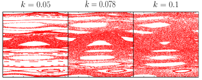
Figure 2: Classical Poincaré sections of 50 trajectories of length $t_{\rm max}=10000$ of the Chirikov typical map for one particular realization of the random phase shifts with $T=10$ and three values: $k=0.05$, $k=0.078$, $k=0.1$. The positions $(\theta_{t},p_{t})\in[0,2\pi[\times[0,2\pi[$ are shown after applications of the full map, i. e. $T$-times iterated typical map with: $t\mod T=0$. The value of the middle figure corresponds to the critical value $k_{c}\approx 0.078$ of (7) for the transition to global diffusive chaos.

It is well known lichtenberg ; chirikov1 ; chirikov2 that the Chirikov criterion of overlapping resonances gives for the Chirikov standard map a numerical value $\pi^{2}/4\approx 2.47$ which is larger than the real critical value $\approx 0.9716$ that is due to a combination of various reasons (effect of second order resonances, finite width of the chaotic layer etc.). However, for the Chirikov typical map these effects appear to be less important, probably due of the random phases in the amplitudes $f_{m}$ and phase shifts of resonance positions. Thus, the expression (7) for the chaos border works quite well including the numerical prefactor, even though the exact value $k_{c}$ depends also on a particular realization of random phases. In Fig. 2 we show the Poincaré sections of the Chirikov typical map for a particular random phase realization for $T=10$ and three different values of $k\in\{0.05,0.078,0.1\}$ where the critical value at $T=10$ is $k_{c}=(\frac{\pi}{2})^{2}\,10^{-3/2}\approx 0.078$. Fig. 2 confirms quite well that the transition to global chaos happens at that value. Actually choosing one particular initial condition $\theta_{0}=0.8\cdot 2\pi$ and $p_{0}=0.25\cdot 2\pi$ one clearly sees that at $k=0.05$ only one invariant curve at $p\approx p_{0}$ is filled and that at $k=0.1$ nearly the full elementary cell is filled diffusively. At the critical value $k=0.078$ only a part of the region $p>p_{0}$ is diffusively filled during a given number of map iterations.

IV Classical diffusion

For $k>k_{c}$ the classical dynamics becomes diffusive in $p_{t}$ and for $k\gg k_{c}$ we can easily evaluate the diffusion constant assuming that the angles $\theta_{t}$ are completely random and uncorrelated. In order to discuss this in more detail we iterate the classical map (3) up to times $t$:

$$p_{t}=p_{0}+k\sum_{\nu=0}^{t-1}\sin(\theta_{\nu}+\alpha_{\nu})$$ (8)

and

$$\theta_{t}=\theta_{0}+\sum_{\mu=1}^{t}p_{\mu}=\theta_{0}+p_{0}\,t+k\sum_{\nu=0}^{t-1}(t-\nu)\,\sin(\theta_{\nu}+\alpha_{\nu})\ .$$ (9)

Using the assumption of random and uncorrelated angles we find that the quantities $\delta p_{t}=p_{t}-p_{0}$ and $\delta\theta_{t}=\theta_{t}-\theta_{0}-p_{0}\,t$ are random gaussian variables (for $t\gg 1$) with average and variance:

$$\langle\delta p_{t}\rangle=\langle\delta\theta_{t}\rangle=0\ ,$$ (10)

$$\langle\delta p_{t}^{2}\rangle=\frac{k^{2}}{2}\,t\quad,\quad\langle\delta\theta_{t}^{2}\rangle=\frac{k^{2}}{12}t(t+1)(2t+1)\approx\frac{k^{2}}{6}\,t^{3}\ ,$$ (11)

implying a diffusive behavior in $p$-space with diffusion constant $D_{0}=(\Delta p)^{2}/\Delta t=k^{2}/2$ which is valid for $k\gg k_{c}$. For $k>k_{c}$ but close to $k_{c}$ we expect the dynamics also to be diffusive but with a reduced diffusion constant $D<D_{0}$ due to correlations of $\theta_{t}$ for different times $t$ and for $k\leq k_{c}$ we have $D=0$. However, we insist that this behavior is expected for long times scales, in particular $t\gg T$ with $T$ being the period of the random phases $\alpha_{\nu}=\alpha_{T+\nu}$. For small times $t\leq T$ there is always, for arbitrary values of $k$ (including the case $k<k_{c}$), a simple short time diffusion with the diffusion constant $D_{0}$ and in this regime Eq. (11) is actually exact (if the average is understood as the average with respect to $\alpha_{\nu}$).

It is interesting to note that Eq. (11) provides an additional way to derive the chaos border $k_{c}$. Actually, we expect the long term dynamics to be diffusive if at the end of the first period $t=T$ the short time diffusion allows to cross at least one resonance in $p$ space : $\delta p_{T}\sim k\sqrt{T}>\Delta p=2\pi/T$ or if the dynamics becomes ergodic in $\theta$ space : $\delta\theta_{T}\sim kT^{3/2}>2\pi$. Both conditions provide the same chaos border $k>k_{c}\sim T^{-3/2}$ exactly confirming the finding of the previous section by the Chirikov criterion of overlapping resonances.

We note that the behavior $\delta\theta_{t}\sim k\,t^{3/2}$ is a direct consequence that $\delta\theta_{t}$ is a sum (integral) over $\delta p_{\mu}$ for $\mu\leq t$ and that $p_{\mu}$ itself is submitted to a diffusive dynamics with $\delta p_{\mu}\sim\mu^{1/2}$. The same type of phase fluctuations also happens in other situations, notably in quantum dynamics where the quantum phase is submitted to some kind of noise with diffusion in energy or in frequency space (with diffusion constant $D_{0}$) implying a dephasing time $t_{\phi}\sim D_{0}^{-1/3}$. For example, a similar situation appears for dephasing time in disordered conductors altshuler where the diffusive energy fluctuations for one-particle states are caused by electron-electron interactions and where the same type of parametric dependence (in terms of the energy diffusion constant) is known to hold. Another example is the adiabatic destruction of Anderson localization discussed in borgonovi where a small noise in the hopping matrix elements of the one-dimensional Anderson model leads to a destruction of localization and diffusion in lattice space because the quantum phase coherence is limited by the same kind of mechanism.

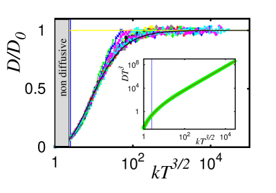
Figure 3: (Color online) The ratio $D/D_{0}$ of the classical diffusion constant $D$ of the Chirikov typical map over the theoretical diffusion constant $D_{0}=k^{2}/2$, assuming perfectly uncorrelated phases $\theta_{t}$, as a function of the scaling parameter $x=kT^{3/2}$ for $10\leq T\leq 1000$ and $T^{-3/2}\leq k\leq 1$. The classical diffusion constant $D$ has been obtained from a linear fit of the average variance $<\delta p_{t}^{2}>$ in the time interval $10\,T\leq t\leq 100\,T$. The average variance has been calculated for 400 different realizations of the random phase shifts and 25 different random initial conditions $(\theta_{0},p_{0})\in[0,2\pi[\times[0,2\pi[$ for each realization. The vertical full (blue) line represents the classical chaos border at $k_{c}T^{3/2}=\pi^{2}/4\approx 2.47$ (compare Fig. 2) and the grey rectangle at the left shadows the non-diffusive regime where the numerical procedure (incorrectly) yields small positive values of $D$ (see text). The full curved (black) line represents the scaling function $D/D_{0}=f(x)$ as given by Eq. (13). The inset shows $DT^{3}$ as a function of the scaling parameter $x=kT^{3/2}$ and the full (red) line represents the scaling function $x^{2}f(x)/2$. The full vertical (blue) line again represents the classical chaos border.

We now turn to the discussion of our numerical study of the classical diffusion in the Chirikov typical map. We have numerically determined the classical diffusion constant for values of $10\leq T\leq 1000$ and $T^{-3/2}\leq k\leq 1$. For this we have simulated the classical map up to times $t\leq 100\,T$ and calculated the long time diffusion constant $D$ as the slope from the linear fit of the variance $\langle\delta p_{t}^{2}\rangle$ for $10\,T\leq t\leq 100\,T$ (in order to exclude artificial effects due to the obvious short time diffusion with $D_{0}=k^{2}/2$). According to Fig. 3 the ratio $D/D_{0}$ can be quite well expressed as a scaling function of the quantity : $kT^{3/2}\sim k/k_{c}$:

$$D\approx D_{0}f\left(kT^{3/2}\right)$$ (12)

where the scaling function $f(x)$ can be approximated by the fit :

$$f(x)=\exp\left(1-\sqrt{1+\frac{18.8}{x}+\frac{23.1}{x^{2}}}\right)\ .$$ (13)

This fit has been obtained from a plot of $\ln(D/D_{0})$ versus $y\equiv x^{-1}$ where the numerical data gives a linear behavior $\ln(D/D_{0})\approx-A_{1}y$ for $y\ll 1$ and $\ln(D/D_{0})\approx-A_{2}y$+const. for $y\gg 1$ with different slopes $A_{1}$ and $A_{2}$ which can be fitted by the ansatz $\ln(D/D_{0})=1-\sqrt{1+C_{1}\,y+C_{2}\,y^{2}}$. The problem to obtain an analytical theory for this scaling function is highly non-trivial and subject to future research. However, we note that the numerical scaling function (13) shows the correct behavior in the limits $x\to\infty$ and $x\to 0$. For $x=k\,T^{3/2}\geq 100$ we have $f(x)\approx 1$ implying $D\approx D_{0}$ for the strongly diffusive regime where phase correlations in $\theta_{t}$ can be neglected. For intermediate values $k_{c}T^{3/2}\approx 2.47<x<100$ there is a two scale diffusive regime with a short time diffusion constant $D_{0}$ for $t\leq T$ and a reduced longer time diffusion constant $D<D_{0}$ for $t\gg T$.

For $k<k_{c}$ ($x<2.47$) the long time diffusion constant is expected to be zero but the numerical fit procedure still results in small positive values (note that the scaling function vanishes very quickly in a non-analytical way $f(x)\sim\exp(-4.8/x)$ as $x\to 0$) simply because here the chosen fit interval $10\,T<t<100\,T$ is too small. In order to numerically identify the absence of diffusion it would be necessary to consider much longer iteration times. We also note that the variance $\langle\delta p_{t}^{2}\rangle$ shows a quite oscillatory behavior for $k<k_{c}$ and $t>T$ indicating the non-diffusive character of the dynamics despite the small positive slope which is obtained from a numerical fit (in a limited time interval). Therefore, we have shadowed in Fig. 3 the regime $x<2.47$ by a grey rectangle in order to clarify that this regime is non-diffusive.

The important conclusion of Fig. 3 is that it clearly confirms the transition to chaotic diffusive dynamics at values $k>k_{c}\sim T^{-3/2}$ and that in addition there is even an approximate scaling behavior in the parameter $x=kT^{3/2}\sim k/k_{c}$.

V Lyapunov exponent and ergodic dephasing time scale

We consider the chaotic regime $k_{c}<k<1$ where the diffusion rate is quite slow and where we expect that the Lyapunov exponent is much smaller than unity implying that the exponential instability of the trajectories develops only after several iterations of the classical map. In order to study this in more detail, we rewrite the map as :

$$p_{t+1}=p_{t}+f_{t}(\theta_{t})\quad,\quad\theta_{t+1}=\theta_{t}+p_{t+1}$$ (14)

where for the Chirikov typical map we have $f_{t}(\theta)=k\cos(\theta+\alpha_{t})$ but in this section we would like to allow for more general periodic kick functions $f_{t}(\theta)$ with vanishing average (over $\theta$). In order to determine the Lyapunov exponent of this map we need to consider two trajectories $(\theta_{t},p_{t})$ and $(\tilde{\theta}_{t},\tilde{p}_{t})$ both being solutions of (14) with very close initial conditions at $t=0$. The differences $\Delta p_{t}=p_{t}-\tilde{p}_{t}$ and $\Delta\theta_{t}=\theta_{t}-\tilde{\theta}_{t}$ are iterated by the following linear map:

$$\Delta p_{t+1}\approx\Delta p_{t}+f_{t}^{\prime}(\theta_{t})\Delta\theta_{t}\quad,\quad\Delta\theta_{t+1}=\Delta\theta_{t}+\Delta p_{t+1}$$ (15)

as long as $|\Delta\theta_{t}|\ll 1$. In a similar way as with the Eqs. (8) and (9) in the last section, we may iterate the linear map up to times $t$ :

$$\Delta p_{t} = \Delta p_{0}+\sum_{\nu=0}^{t-1}f_{\nu}^{\prime}(\theta_{\nu})\Delta\theta_{\nu}\ ,$$ (16)

$$\Delta\theta_{t} = \Delta\theta_{0}+\sum_{\mu=1}^{t}\Delta p_{\mu}$$ (17)

$$= \Delta\theta_{0}+t\,\Delta p_{0}+\sum_{\nu=0}^{t-1}(t-\nu)\,f_{\nu}^{\prime}(\theta_{\nu})\,\Delta\theta_{\nu}\ .$$

We now assume that in the chaotic regime the phases $\theta_{\nu}$ are random and uncorrelated, and that the average of the squared phase difference behaves as :

$$\langle\Delta\theta_{t}^{2}\rangle=\Theta(t)\,\Delta\theta_{0}^{2}$$ (18)

with a smooth function $\Theta(t)$ we want to determine. From Eq. (17) we obtain in the continuum limit the following integral equation for the function $\Theta(t)$ :

$$\Theta(t)=1+2A\,t+A^{2}\,t^{2}+\kappa\int_{0}^{t}(t-\nu)^{2}\Theta(\nu)\,d\nu$$ (19)

where $\kappa=\langle f_{\nu}^{\prime}(\theta)^{2}\rangle_{\theta}$ and $A=\Delta p_{0}/\Delta\theta_{0}$. For the map (3) we have $\kappa=k^{2}/2$. This integral equation implies the differential equation

$$\Theta^{\prime\prime\prime}(t)=2\kappa\,\Theta(t)$$ (20)

with the general solution :

$$\Theta(t)=\sum_{j=1}^{3}C_{j}\,e^{2\lambda_{j}\,t}$$ (21)

where the constants $C_{j}$ are determined by the initial conditions at $t=0$ and $2\lambda_{j}$ are the three solutions of $(2\lambda_{j})^{3}=2\kappa$ :

$$\lambda_{1}=(2\kappa)^{1/3}/2\quad,\quad\lambda_{2}=e^{2\pi i/3}\lambda_{1}\quad,\quad\lambda_{3}=\lambda_{2}^{*}\ .$$ (22)

Since only $\lambda_{1}$ has a positive real part, we have in the long time limit :

$$\Theta(t)\approx C_{1}\,e^{2\lambda_{1}\,t}$$ (23)

and therefore by Eq. (18) $\lambda_{1}$ represents approximately the Lyapunov exponent of the map (14).

We note that this calculation of the Lyapunov exponent is not exact, essentially because we evaluate the direct average $\langle\Delta\theta_{t}^{2}\rangle$ instead of $\exp(\langle\ln(\Delta\theta_{t}^{2})\rangle)$. A proper and more careful evaluation of the Lyapunov exponent for this kind of maps (in the regime $\kappa\ll 1$, assuming chaotic behavior with uncorrelated phases) has been done by Rechester et al. rechester in the context of a motion along a stochastic magnetic field. Their result reads in our notations :

$$\lambda=\frac{3^{1/3}\,\Gamma(\frac{5}{3})}{4\,\Gamma(\frac{4}{3})}\,\kappa^{1/3}\approx 0.36\,\kappa^{1/3}\approx 0.29k^{2/3}$$ (24)

while from Eq. (22) we have $\lambda_{1}\approx 0.63\,\kappa^{1/3}$ with the same parametric dependence but with a different numerical prefactor. The dependence (24) has been confirmed in numerical simulations chi1981 for the model (3) and we do not perform numerical simulations for $\lambda$ here. We note that in the map (3) the Lyapunov exponent $\lambda$ gives the Kolmogorov-Sinai entropy lichtenberg .

The inverse of the Lyapunov exponent defines the Lyapunov time scale $t_{\rm Lyap}\sim\kappa^{-1/3}$ which is the time necessary to develop the exponential instability of the chaotic motion. According to Eq. (11) we also have : $\langle\delta\theta_{t}^{2}\rangle=D_{0}\,t^{3}/3$ with $D_{0}=\langle f_{\nu}(\theta)^{2}\rangle_{\theta}$ implying an ergodic dephasing time $t_{\Phi}\sim D_{0}^{-1/3}$ being the time necessary for a complete dephasing where there is no correlation of the actual phase $\theta_{t}$ with respect to the ballistic phase $\theta_{\rm ball.}=\theta_{0}+p_{0}\,t$. For the Chirikov typical map with $f_{\nu}(\theta)=k\,\sin(\theta+\alpha_{\nu})$ the averages of $f_{\nu}^{\prime}(\theta)^{2}$ and $f_{\nu}(\theta)^{2}$ are identical, implying $\kappa=D_{0}=k^{2}/2$, and these two time scales coincide : $t_{\rm Lyap}=t_{\Phi}\sim k^{-2/3}$. Furthermore, the condition for global chaos, $k>k_{c}\sim T^{-3/2}$, reads $t_{\rm Lyap}=t_{\Phi}<T$ implying that the exponential instability and complete dephasing must happen before the period $T$.

We mention that for other type of maps, in particular if $f_{\nu}(\theta)$ contains higher harmonics such as $\ \sin(M\theta)\$ we may have : $\kappa\sim M^{2}D_{0}$, and therefore parametrically different times scales $t_{\rm Lyap}\sim M^{-2}\,t_{\Phi}$. Examples of these type of maps have been studied in Ref. rechester and also in Refs. frahm1 ; frahm1a in the context of angular momentum diffusion and localization in rough billiards.

For the Chirikov typical map there is a further time scale $t_{\rm Res}$ which is the time necessary to cross one resonance of width $\Delta p=2\pi/T$ by the diffusive motion $\langle\delta p_{t}^{2}\rangle=k^{2}\,t/2$ :

$$t_{\rm Res}\sim\frac{1}{(kT)^{2}}\sim k^{-2/3}\,\left(\frac{k}{k_{c}}\right)^{-4/3}\sim t_{\Phi}\,\left(\frac{k}{k_{c}}\right)^{-4/3}\quad.$$ (25)

In the chaotic regime $k>k_{c}$ this time scale is parametrically smaller than the dephasing time and the Lyapunov time scale.

VI Quantum evolution

We now study the quantum evolution which is described by the quantum map (4) (see section II). Typically in the literature studying the quantum version of Chirikov standard map the value of $\hbar$ is absorbed in a modification of the elementary kick period and the kick parameter $k$. Here we prefer to keep $\hbar$ as an independent parameter (also for the numerical simulations) and to keep the notation $T$ of the (integer) period of the time dependent kick-angle $\alpha(t)$. In this way we clearly identify two independent classical parameters $k$ and $T$, one quantum parameter $\hbar$ and a numerical parameter $N\gg 1$ being the finite dimension of the Hilbert space for the numerical quantum simulations. For the physical understanding and discussion it is quite useful to well separate the different roles of these parameters and we furthermore avoid the need to translate between “classical” and “quantum” versions of the kick strength $k$.

We choose the Hilbert space dimension to be a power of 2 : $N=2^{L}$ allowing an efficient use of the discrete fast Fourier transform (FFT) in order to switch between momentum and position (phase) representation. A state $|\psi\rangle$ is represented by a complex vector with $N$ elements $\psi(j)$, $j=0,\ldots,N-1$ where $p_{j}=\hbar j$ are the discrete eigenvalues of the momentum operator $\hat{p}$. In order to apply the map (4) to the state $|\psi\rangle$ we first use an inverse FFT to transform to the phase representation in which the operator $\hat{\theta}$ is diagonal with eigenvalues $\theta_{j}=2\pi j/N$, $j=0,\ldots,N-1$, then we apply the first unitary matrix factor in (4) which is diagonal in this base, we apply an FFT to go back to the momentum representation and finally the second unitary matrix factor, diagonal in the momentum representation, is applied. This procedure can be done with ${\cal O}(N\log_{2}(N))$ operations (for the FFT and its inverse) plus ${\cal O}(N)$ operations for the application of the diagonal unitary operators.

We have also to choose a numerical value of $\hbar$ and this depends on which kind of regime (semiclassical regime or strong quantum regime) we want to investigate. We note that due to the dimensional cut off we obtain a quantum periodic boundary condition : $\psi(0)=\psi(N)$, i. e. the quantum dynamics provides in $p$ representation always a momentum period of $\hbar N$. Furthermore the classical map is also periodic in momentum with period $2\pi$ and it is possible to restrict the classical momentum to one elementary cell where the momentum is taken modulo $2\pi$. Therefore one plausible choice of $\hbar$ amounts to choose the quantum period $\hbar N$ to be equal to the classical period $2\pi$, i. e.: $\hbar=2\pi/N$. In this case the quantum state covers exactly one elementary cell in phase space. Since $\hbar\to 0$ for $N\to\infty$, we refer to this choice as the semiclassical value of $\hbar$.

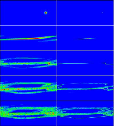
Figure 4: (Color online) Quantum evolution of the Chirikov typical map at $k=0.1$ and $T=10$ in the semiclassical limit with $\hbar=2\pi/N$ and with the Hilbert space dimension $N=2^{12}$ (left column) and $N=2^{16}$ (right column) at times $t=0$ (first row), $t=20$ (second row), $t=60$ (third row), $t=100$ (fourth row) and $t=150$ (fifth row). Shown are Husimi functions with maximum values at red (grey), intermediate values at green (light grey) and minimum values at blue (black) at the lower half of one elementary cell $\theta\in[0,2\pi[$, $p\in[0,\pi[$. The initial condition is a coherent gaussian state centered at $\theta_{0}=0.8\cdot 2\pi$ and $p_{0}=0.25\cdot 2\pi$ with a variance (in $p$-representation) of $\Delta p=2\pi/\sqrt{12N}$. The resolution corresponds to $\sqrt{N}$ (64 or 256) squares in one line. The realization of the random phase shifts is identical to that of Fig. 2. Note that at the considered value $k=0.1$ the global classical dynamic is diffusive but requires iteration times of $t\sim 10000$ to fill one elementary cell (see Fig. 5).

In this section, we present some numerical results of the quantum dynamics using the semiclassical value of $\hbar$. In Fig. 4, we show the Husimi functions for the case $T=10$, $k=0.1$ with an initial state being a minimal gaussian wave packet centered at $\theta_{0}=0.8\cdot 2\pi$ and $p_{0}=0.25\cdot 2\pi$ with a variance (in $p$-representation) of $\Delta p=2\pi/\sqrt{12N}$. This position is well inside a classically chaotic region (see Fig. 2). The Hilbert space dimensions $N$ are $2^{12}$ and $2^{16}$ and the iteration times are $t\in\,\{0,\,20,\,60,\,100,\,150\}$. We see that at these time scales the motion extends to two classical resonances with two stable and quite large islands. For $N=2^{12}$ the classical phase space structure is quite visible but the finite “resolution” in phase space due to quantum effects is quite strong while for $N=2^{16}$ the Husimi function allows to resolve much better smaller details of the classical motion. We note that the Husimi function is obtained by smoothing of the Wigner function over a phase space cell of $\hbar$ size (see e.g. more detailed definitions and Refs. in frahm2 ).

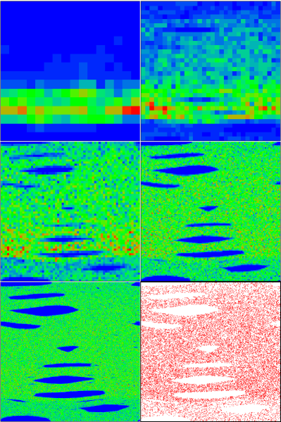
Figure 5: (Color online) Quantum evolution of the Chirikov typical map as in Fig. 4 with the same coherent gaussian state as initial condition, same values $k=0.1$ and $T=10$, $\hbar=2\pi/N$ but at the iteration time $t=20000$ and at different values of $N=2^{8}$, $N=2^{10}$ (first row), $N=2^{12}$, $N=2^{14}$ (second row), $N=2^{16}$ and classical simulation (third row). For the classical map 20000 trajectories have been iterated up to the same time $t=20000$ with random initials conditions very close to the initial position at $\theta_{0}=0.8\cdot 2\pi\pm 0.002$ and $p_{0}=0.25\cdot 2\pi\pm 0.002$. Colors are as in Fig. 4.

We note that for $T=10$ the value of the kick strength $k=0.1$ is only slightly above the chaos border $0.078$ with global diffusion but there are still large stable islands that occupy a significant fraction of the phase space. At this value the numerically computed diffusion constant is $D=0.1D_{0}\approx 1/2000$ (see section III and Fig. 3). In Fig. 5 we compare the Husimi functions for various Hilbert space dimensions at time $t=20000$. This time is sufficiently long so that a diffusive spreading in $p$-space gives $\delta p_{t}=\sqrt{Dt}\approx 3.162$ thus roughly covering one elementary cell (but not absolutely uniformly).

For the smallest value of $N=2^{8}$ we observe a very strong influence of quantum effects with a Husimi function extended to half an elementary cell which is significantly stronger localized (in the momentum direction) than the diffusive classical spreading would suggest. Furthermore we cannot identify any classical phase space structure. This is quite normal due to the very limited resolution of $\sqrt{N}=16$ “quantum-pixels” in both directions of $\theta$ and $p$. For $N=2^{10}$ the quantum effects are still strong but the Husimi function already extends to $~{}85$% of the elementary cell and we can identify first very slight traces of at least three large stable islands. For $N=2^{12}$ the Husimi function fills the elementary cell as suggested by the classical spreading but the distribution is less uniform than for larger values of $N$ or for the classical case. We can also quite well identify the large scale structure of the phase space with the main stable islands associated to each resonance. However, the fine structure of phase space is not visible due to quantum effects. For $N=2^{14}$ and even more for $N=2^{16}$, the resolution of the Husimi function increases and approaches the classical distribution which is also shown in Fig. 5 for comparison. For $N=2^{16}$, we even see first traces of small secondary islands that are not associated to the main resonances. We note that the classical distribution in Fig. 5 is not a full phase portrait (showing “all” iteration times) but it only contains the classical positions after $t=20000$ iterations with random initial positions : $\theta_{0}=0.8\cdot 2\pi\pm 0.002$, $p_{0}=0.25\cdot 2\pi\pm 0.002$ close to the gaussian wave packet used as initial state in Figs. 4, 5.

Finally we note that a wave packet with initial size $\delta\theta_{0}\approx\sqrt{\hbar}$ grows exponentially with time and spreads over the whole phase interval $2\pi$ after the Ehrenfest time scale chi1981 ; zasl ; chi1988

$$t_{\rm E}\approx\ln(2\pi/\sqrt{\hbar})/\lambda.$$ (26)

For the parameters of Fig. 4, e.g. $\hbar=2\pi/2^{16}$, this gives $t_{\rm E}\approx 103$ that is in agreement with the numerical data showing that the spearing in phase reaches $2\pi$ approximately at $t=100$.

In summary the quantum simulation of the Chirikov typical map using the semiclassical value $\hbar=2\pi/N$ reproduces quite well the classical phase space structure for sufficiently large $N$ while for smaller values of the Hilbert space dimension ($N\leq 2^{8}$) the nature of motion remains strongly quantum and the diffusive spreading over the cell is stopped by quantum localization.

VII Chirikov Localization

It is well established chidls ; dls1986 that, in general, quantum maps on one-dimensional lattices, whose classical counterpart is diffusive with diffusion constant $D_{\rm cl}$, show dynamical exponential localization of the eigenstates of the unitary map operator with the localization length $\ell_{0}=D_{\rm cl.}/\hbar^{2}$ measured in number of lattice sites (that corresponds to the quantum number $n$ associated to the momentum by $p=\hbar n$). Here $D_{\rm cl.}$ is the diffusion rate in action per period of the map. This expression for $\ell_{0}$ is valid for the unitary symmetry class which applies to the Chirikov typical map which is not symmetric with respect to the transformation $\theta\to-\theta$. We have furthermore to take into account that the map (4) depends on time due to the random phases $\alpha_{\nu}$ and in order to determine the localization length we have to use the diffusion constant for the full $T$-times iterated map (which does not depend on time) : $D_{\rm cl.}=D_{0}\,T$ assuming we are in the regime where $D=D_{0}$ for $k\gg k_{c}$. In this case we expect a localization length

$$\ell_{0}=\frac{D_{0}\,T}{\hbar^{2}}=\frac{k^{2}\,T}{2\hbar^{2}}\ .$$ (27)

This localization length is obtained as the exponential localization length from the eigenvectors of the full ($T$-times iterated) unitary map operator. In numerical studies of the Chirikov typical map it is very difficult and costly to access to these eigenvectors and we prefer to simply iterate the quantum map with an initial state localized at one momentum value in $p$-representation and to measure the exponential spreading of $|\psi(t)\rangle$ at sufficiently large times (using time and ensemble average). This procedure is known dls1986 to provide a localization length $\ell$ artificially enhanced by a factor of two: $\ell=2\ell_{0}$.

Let us note that the relation (27) assumes that the classical dynamics is chaotic and is characterized by the diffusion $D_{0}$. It also assumes that the eigenvalues of the unitary evolution operator are homogeneously distributed on the unitary circle. For certain dynamical chaotic systems the second condition can be violated giving rise to a multifractal spectrum and delocalized eigenstates (this is e.g. the case of the kicked Harper model lima ; prosen ). The analytical derivation of (27) using supersymmetry field theory assumes directly frahm1a or indirectly zirnb that the above second condition is satisfied. We also assume that this condition is satisfied due to randomness of $\alpha_{t}$ phases in the map (3).

Before we discuss our numerical results for the localization length we would like to remind the phenomenological argument coined in chi1981 which allows to determine the above expression relating localization length to the diffusion constant and which we will below refine in order to take into account the two-scale diffusion with different diffusion constants at short and long time scales.

Suppose that the classical spreading in $p$-space is given by a known function :

$$P_{2}(t)=\langle\delta p_{t}^{2}\rangle$$ (28)

where $P_{2}(t)$ is a linear function for simple diffusion but it may be more general in the context of this argumentation (but still below the ballistic behavior $t^{2}$ for $t\to\infty$). For the quantum dynamics we choose an initial state localized at one momentum value. This state can be expanded using $\ell$ eigenstates of the full map operator with a typical eigenphase spacing $2\pi/\ell$. The iteration time $t$ (with $t$ being an integer multiple of $T$) corresponds to $t/T$ applications of the full map operator. We expect the quantum dynamics to follow the classical spreading law (28) for short time scales such that we cannot resolve individual eigenstates of the full map operator, i. e. for $2\pi t/(T\ell)<2\pi$. Therefore at the critical time scale $t^{*}=\ell T$ we expect the effect of quantum localization to set in and to saturate the classical spreading at the value $\delta p_{\rm loc.}^{2}\sim\hbar^{2}\ell^{2}$ due to the finite localization length $\ell$ (measured in integer units of momentum quantum numbers). This provides an implicit equation for $t^{*}$ :

$$\left(\frac{t^{*}}{T}\right)^{2}=\ell^{2}=C\frac{P_{2}(t^{*})}{\hbar^{2}}$$ (29)

where $C$ is a numerical constant of order unity. Let us first consider the case of simple diffusion with constant $D_{0}$ for which we have $P_{2}(t)=D_{0}\,t$. In this case we obtain :

$$\ell=\frac{t^{*}}{T}=C\frac{D_{0}\,T}{\hbar^{2}}=C\ell_{0}$$ (30)

with $\ell_{0}$ given by Eq. (27). This result provides the numerically measured value $\ell=2\ell_{0}$ by the exponential spreading of $|\psi(t)\rangle$ if we choose $C=2$. Below we will also apply Eq. (29) to the case of two scale diffusion with different diffusion constants at short and long time scales providing a modified expression for the localization length.

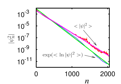
Figure 6: (Color online) Illustration of the Chirikov localization for the quantum Chirikov typical map. Shown is the (averaged) absolute squared wave function in $p$-representation as a function of the integer quantum number $n$ associated to $p=\hbar n$. The initial state at $t=0$ is localized at $n=0$ and the quantum typical map has been applied up to times $t=t_{\rm max}$ with $t_{\rm max}$ chosen such that the initial classical diffusion is well saturated at $t_{\rm max}/4$ due to quantum effects (see Fig. 7). In order to determine numerically the localization length, first $|\psi_{n}|^{2}$ has been time-averaged for the time interval $t_{\rm max}/4\leq t\leq t_{\rm max}$ and then a further ensemble average (over 100 realizations of the random phase shifts) of $|\psi_{n}|^{2}$ (upper red/gray curve) or of $\ln(|\psi_{n}|^{2})$ (lower blue/black curve) has been applied. The localization lengths are obtained as the (double) inverse slopes of a linear fit (with relative weights $w_{n}\sim|\psi_{n}|^{2}$) of $\ln(|\psi_{n}|^{2})$ versus $n$. Here the parameters are: $N=2^{12}$, $k=0.5$, $T=100$, $t_{\rm max}=546132$, $\hbar=2\pi/(17+\gamma)\approx 0.357$ with the golden number $\gamma=(\sqrt{5}-1)/2\approx 0.618$. The fits are given by the thick straight lines. The theoretical localization length is $\ell_{0}=k^{2}T/(2\hbar^{2})\approx 98.3$ while the numerical fits provide $\ell_{\psi}\approx 231.7$ (upper curve) and $\ell_{\ln\psi}\approx 187.5$ (lower curve).

First we want to present our numerical results for the localization length of the quantum Chirikov typical map. Since the localization length scales as $\hbar^{-2}$ we cannot use the semiclassical value $\hbar=2\pi/N$ since in the limit $N\to\infty$ the localization length would always be larger than $N$ and in addition we would only cover one elementary classical cell of phase space which is not very suitable to study the effects of diffusion and localization in momentum space. Therefore we choose a finite and fixed value $\hbar=2\pi/(\tilde{N}+\gamma)$ where $\tilde{N}$ is some fixed integer in the range $1\ll\tilde{N}\ll N$ and $\gamma=(\sqrt{5}-1)/2\approx 0.618$ is the golden number because we want to avoid artificial resonance effects between the classical momentum period $2\pi$ and the quantum period $\hbar N$ (due to the finite dimensional Hilbert space). The ratio of these two periods, $N/(\tilde{N}+\gamma)\gg 1$, is roughly the number of elementary classical cells covered by the quantum simulation. For most simulations we have chosen $\tilde{N}=17$ and varied the classical parameters $k$ and $T$ but we also provide the data for a case where the values of $k$ and $T$ are fixed and $\tilde{N}$ varies.

For the numerical quantum simulation we choose the initial state $|\psi(0)\rangle=|0\rangle$ being perfectly localized in momentum space and we apply the quantum Chirikov typical map up to a sufficiently large time scale $t_{\rm max}$ chosen such that the initial diffusion is well saturated at $t_{\rm max}/4$ and we perform a time average of $|\psi_{n}|^{2}=|\langle n|\psi\rangle|^{2}$ for the time interval $t_{\rm max}/4\leq t\leq t_{\rm max}$. The resulting time average is furthermore averaged with respect to different realizations of the $T$ random phases $\alpha_{\nu}$ and here we consider two cases where we average either $|\psi_{n}|^{2}$ or $\ln(|\psi_{n}|^{2})$. We then determine two numerical values $\ell_{\psi}$ and $\ell_{\ln\psi}$ by a linear fit of $\ln(|\psi_{n}|^{2})=2n/\ell+$const. with relative weight factors $w_{n}\sim|\psi_{n}|^{2}$ in order to emphasize the initial exponential decay and to avoid problems at large values of $n$ where the finite numerical precision ($\sim 10^{-15}$) or the finite value of $N$ may create an artificial saturation of the exponential decay. This procedure is illustrated in Fig. 6 for the parameters $k=0.5$, $T=100$, $\hbar=2\pi/(17+\gamma)$ and $N=2^{12}$. We see that the two numerical values $\ell_{\psi}$ and $\ell_{\ln\psi}$ are roughly $2\ell_{0}$ as expected but may differ among themselves by a modest numerical factor.

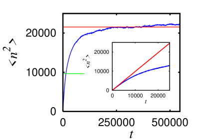
Figure 7: (Color online) The ensemble averaged variance of the expectation value of $n^{2}$ as a function of $t$ for the same parameters (and the same realizations of the random phase shifts) as in Fig. 6. The upper horizontal (red) line corresponds to the saturation value $\ell_{\rm diff}^{2}$ (obtained from a time average of $<n^{2}>$ in the interval $t_{\rm max}/4\leq t\leq t_{\rm max}$) with $\ell_{\rm diff}\approx 146.8$ being the localization due to saturation of diffusion. The short lower horizontal (green) line corresponds to $\ell_{0}^{2}$ with the theoretical localization length $\ell_{0}\approx 98.3$ (see also Fig. 6). The inset shows the initial diffusive regime at shorter time scales. The straight (red/grey) line shows the value $D_{0}/\hbar^{2}\approx 0.983$ associated to the initial diffusion: $\hbar^{2}\langle n^{2}\rangle=\langle p^{2}\rangle\approx D_{0}\,t$ and with the theoretical diffusion constant $D_{0}=k^{2}/2$.

The localization length can also be determined from the saturation of the diffusive spreading which gives a localization length $\ell_{\rm diff}$ where $\ell_{\rm diff}^{2}$ is the time average of the quantum expectation value $\langle n^{2}\rangle$ for the interval $t_{\rm max}/4\leq t\leq t_{\rm max}$ (see Fig. 7). Typically $\ell_{\rm diff}$ is comparable to $\ell_{\psi}$ and $\ell_{\ln\psi}$ up to a modest numerical factor.

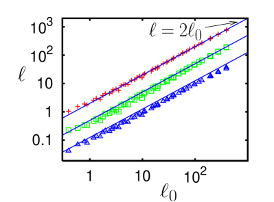
Figure 8: (Color online) Localization length determined by three different numerical methods as a function of the theoretical value $\ell_{0}=k^{2}T/(2\hbar^{2})$ in a double logarithmic representation. The data points correspond to $\ell_{\psi}$ (red crosses) obtained from a linear fit of $\ln\langle|\psi_{n}|^{2}\rangle$ versus $n$ (see Fig. 6), $\ell_{\ln\psi}$ (green squares) obtained from a linear fit of $\langle\ln|\psi_{n}|^{2}\rangle$ versus $n$, $\ell_{\rm diff}$ (blue triangles) obtained from the saturation of quantum diffusion (see Fig. 7). The straight full (blue) line represents $\ell=2\ell_{0}$. For clarity the data points for $\ell_{\ln\psi}$ (or $\ell_{\rm diff}$) have been shifted down by a factor of 4 (or 16). The value $\hbar=2\pi/(17+\gamma)\approx 0.357$ is exactly as in Fig. 6 while $k\in\{0.1,0.15,0.2,0.3,0.5,0.7,1.0\}$ and $T\in\{10,15,20,30,50,70,100\}$. The Hilbert space dimension is mostly $N=2^{12}$ except for a few data points with the largest values of $\ell_{0}$ where we have chosen $N=2^{14}$. The ensemble averages have been performed over 100 different realizations of the random phase shifts.

In Fig. 8, we compare the three numerically calculated values of the localization $\ell_{\psi}$, $\ell_{\ln\psi}$ and $\ell_{\rm diff}$ with the theoretical expression $\ell_{0}=D_{0}\,T/\hbar^{2}$ for various values of the classical parameters : $k\in\{0.1,0.15,0.2,0.3,0.5,0.7,1.0\}$ and $T\in\{10,15,20,30,50,70,100\}$ and for the fixed value $\hbar=2\pi/(17+\gamma)\approx 0.357$. We see that $\ell_{\psi}$ agrees actually very well with $2\ell_{0}$ for a wide range of parameters and three orders of magnitude variation. For $\ell_{\ln\psi}$ and $\ell_{\rm diff}$ the values are somewhat below $2\ell_{0}$ with a modest numerical factor (about 1.5 or smaller) but the overall dependence on the parameters is still correct on all scales.

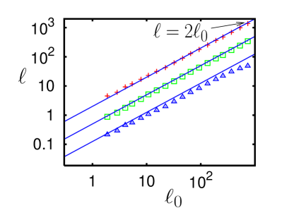
Figure 9: (Color online) Same as in Fig. 8 but with fixed values for the classical parameters $k=0.2$ and $T=50$ while $\hbar=2\pi/(\tilde{N}+\gamma)$ varies with the integer variable $\tilde{N}$ in the interval $8\leq\tilde{N}\leq 200$ (i. e.: $0.03132\leq\hbar\leq 0.7291$). The number of realizations of the random phase shifts is 20.

In Fig. 9, we present a similar comparison as in Fig. 8, but here we have fixed the classical parameters to $k=0.2$ and $T=50$ and we vary $\hbar=2\pi/(\tilde{N}+\gamma)$ with $8\leq\tilde{N}\leq 200$ i. e.: $0.03132\leq\hbar\leq 0.7291$. Again there is very good agreement of $\ell_{\psi}$ and $\ell_{\ln\psi}$ with $2\ell_{0}$ for nearly three orders of magnitude while for $\ell_{\rm diff}$ there is slight decrease for larger values of $\ell_{0}$.

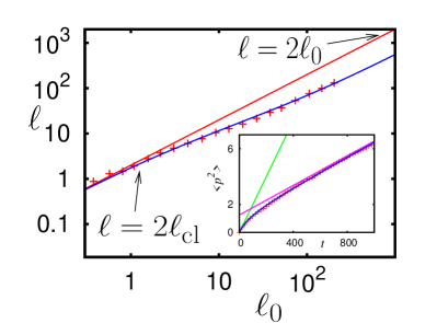
Figure 10: (Color online) The localization length $\ell=\ell_{\psi}$ versus the theoretical value $\ell_{0}=k^{2}T/(2\hbar^{2})$ for $k=0.2$, $T=10$ and the same values of $\hbar$ as in Fig. 9. The straight full (red) upper line corresponds to $\ell=2\ell_{0}$. The lower full (blue) curve corresponds to the corrected expression $\ell=2\ell_{\rm cl}(\ell_{0})=2\ell_{0}/\left[h(\ell_{0})+\sqrt{h(\ell_{0})^{2}+2B\ell_{0}}\right]$, $h(\ell_{0})=(1-2A\ell_{0})/2$, $A\approx 0.03121$, and $B\approx 0.1177$ due to a modified classical dynamics (see text for explanation). The number of random phase realizations is 50. The inset shows the classical diffusion for the same classical parameters $k=0.2$, $T=10$. The data points (red crosses) are (selected) numerical data and the full (blue/black) curve represents the numerical fit: $\langle p^{2}\rangle=D_{0}\,t\,(T+At)/(T+Bt)$ providing the two parameters $A$ and $B$ for the corrected localization length $\ell_{\rm cl}$ in the main figure. The two straight lines correspond to the initial diffusion at short time scales with diffusion constant $D_{0}=k^{2}/2$ and the final diffusion at long time scales with $D=D_{0}\,(A/B)\approx 0.2652\,D_{0}$. This value of $D$ coincides quite well with the value of the scaling curve in Fig. 3 at $x=kT^{3/2}\approx 6.32$.

The agreement $\ell_{\psi}\approx 2\ell_{0}=2D_{0}\,T/\hbar^{2}$ in Fig. 8 for a very large set of classical parameters is actually too perfect because some of the data points fall in the regime where the scaling parameter $x=kT^{3/2}$ is relatively small (between 2.47 and 30) with a classical diffusion constant $D$ well below its theoretical value $D_{0}=k^{2}/2$ (see Fig. 3). Therefore one should expect that the localization length is reduced as well according to $\ell\approx 2D\,T/\hbar^{2}<2\ell_{0}$ but the numerical data in Fig. 8 do not at all confirm this reduction of the localization length we would expect from a classically reduced diffusion constant. One possible explanation is that the classical mechanism of relatively strongly correlated phases which induces the reduction of the diffusion constant depends on the fine structure of the classical dynamics of the Chirikov typical map in phase space, a fine structure which the quantum dynamics may not resolve if the value of $\hbar$ is not sufficiently low. Therefore the classical phase correlations are destroyed in the quantum simulation and we indeed observe the localization length $\ell=2\ell_{0}$ using the theoretical value of the diffusion constant $D_{0}$ and not the reduced diffusion constant $D$.

In order to investigate this point more thoroughly one should therefore vary $\hbar$ in order to see if it is possible to see this reduction of the diffusion constant also in the localization length provided that $\hbar$ is small enough. In Fig. 9, we have indeed data points with smaller values of $\hbar$ but here the classical parameters $k=0.2$ and $T=50$ still provide a large scaling parameter $k\,T^{3/2}\approx 70.7$ with a diffusion constant $D\approx 0.9\,D_{0}$ already quite close to $D_{0}$. In Fig. 10, we therefore study the same values of $\hbar$ (as in Fig. 9) but with modified classical parameters $k=0.2$ and $T=10$ such that $k\,T^{3/2}\approx 6.32$ resulting in a diffusion constant $D=0.2859\,D_{0}$ well below $D_{0}$. In Fig. 10, we indeed observe that the localization length $\ell_{\psi}$ is significantly below $2\ell_{0}$ for larger values of $\ell_{0}$ (small values of $\hbar$).

We can actually refine the theoretical expression of the localization length in order to take into account the reduction of the diffusion constant. For this, we remind that for short time scales $t\leq T$ the initial diffusion is always with $D_{0}$ and that only for $t\gg T$ we observe the reduced diffusion constant $D$. We have therefore applied the following fit :

$$P_{2}(t)=D_{0}\,t\,\frac{T+A\,t}{T+B\,t}$$ (31)

to the classical spreading where $A$ and $B$ are two fit parameters. This expression fits actually very well the classical two scale diffusion with $D_{0}$ for short time diffusion and with $D=D_{0}(A/B)$ for the long time diffusion. For $k=0.2$ and $T=10$ we obtain (see inset of Fig. 10) the values $A\approx 0.03121$ and $B\approx 0.1177$ implying $D=D_{0}\,(A/B)\approx 0.2652\,D_{0}$ which is only slightly below the above value $D=0.2859\,D_{0}$ (obtained from the linear fit of the classical spreading for the interval $10\,T<t<100\,T$). We can now determine a refined expression of the localization length using the two scale diffusion fit (31) together with the implicit equation (29) for the critical time scale $t^{*}$ which results in the following equation for $\ell$ :

$$\ell^{2}=2\frac{P_{2}(\ell T)}{\hbar^{2}}=2\,\ell_{0}\,\ell\frac{1+A\ell}{1+B\ell}\ .$$ (32)

This is simply a quadratic equation in $\ell$ whose positive solution can be written in the form :

$$\ell=2\ell_{cl}(\ell_{0})=\frac{2\ell_{0}}{h(\ell_{0})+\sqrt{h(\ell_{0})^{2}+2B\ell_{0}}}$$ (33)

with $h(\ell_{0})=(1-2\,A\ell_{0})/2$. One easily verifies that the limit $D=D_{0}$, which corresponds to $A=B$, immediately reproduces $\ell_{\rm cl}(\ell_{0})=\ell_{0}$ as it should be. Furthermore, the limit $\ell_{0}A\gg 1$ (i.e. : $\hbar\ll\sqrt{D_{0}\,T/A}$) provides $\ell_{\rm cl}(\ell_{0})\approx\ell_{0}(A/B)$ while for $\ell_{0}A\ll 1$ we have $\ell_{\rm cl}(\ell_{0})\approx\ell_{0}$ (even for $A\neq B$).

The data points of $\ell_{\psi}$ in Fig. 10 coincide very well with the refined expression (33) thus clearly confirming the influence of the classical two scale diffusion on the value of the localization length as described by Eq. (33). Depending on the values of $\hbar$ the refined localization length $\ell_{\rm cl}(\ell)$ is either given by $\ell_{0}$ if $\hbar\gg\sqrt{D_{0}\,T/A}$ or by the reduced value $\ell_{0}(A/B)$ if $\hbar\ll\sqrt{D_{0}\,T/A}$. In the first case we do not see the effect of the reduced diffusion constant because the value of $\hbar$ is too large to resolve the subtle fine structure of the classical dynamics. Furthermore the critical time scale $t^{*}$, where the localization sets in, is below $T$ and the momentum spreading saturates already in the regime of the initial short time diffusion with $D_{0}$. In the second case $\hbar$ is small enough to resolve the fine structure of the classical dynamics and the time scale $t^{*}$ is above $T$ such that we may see the reduced diffusion constant $D=D_{0}(A/B)$ leading to the reduced localization length $\ell_{\rm cl}(\ell_{0})=\ell_{0}(A/B)$.

VIII Discussion

In this work we analyzed the properties of classical and quantum Chirikov typical map. This map is well suited to describe systems with continuous chaotic flow. For the classical dynamics our studies established the dependence of diffusion and instability on system parameters being generally in agreement with the first studies presented in chirikov1 ; rechester ; chi1981 . In the quantum case we showed that the chaotic diffusion is localized by quantum interference effects giving rise to the Chirikov localization of quantum chaos. We demonstrated that the localization length is determined by the diffusion rate in agreement with the general theory of Chirikov localization developed in chi1981 ; prange ; chidls ; dls1986 . The Chirikov typical map has more rich properties compared to the Chirikov standard map and we think that it will find interesting applications in future.

References

- (1) A. Lichtenberg and M. Lieberman, Regular and Chaotic Dynamics, Springer, N.Y. (1992).
- (2) B.V. Chirikov, “Research concerning the theory of nonlinear resonance and stochasticity”, Preprint N 267, Institute of Nuclear Physics, Novosibirsk (1969) [translation: CERN Trans. 71 - 40, Geneva, October (1971)].
- (3) B. V. Chirikov, Phys. Rep. 52, 263 (1979).
- (4) B. Chirikov and D. Shepelyansky, Scholarpedia 3(3):3550 (2008).
- (5) G.Casati, B.V.Chirikov, J.Ford and F.M.Izrailev, Lect. Notes Phys. (Springer) 93, 334 (1979).
- (6) B. V. Chirikov, F. M. Izrailev and D. L. Shepelyansky, Sov. Scient. Rev. C 2, 209 (1981).
- (7) B. V. Chirikov and D. L. Shepelyansky, Izv. Vyss. Ucheb. Zav. Radiofizika 29, 1041 (1986).
- (8) D. L. Shepelyansky, Phys. Rev. Lett. 56, 677 (1986); Physica D 28, 103 (1987).
- (9) S. Fishman, D.R. Grempel and R.E Prange, Phys. Rev. Lett. 49, 509 (1982).
- (10) S. Fishman, in Quantum Chaos: E.Fermi School Course CXIX, G. Casati, I. Guarneri and U. Smilansky (Eds.), North-Holland, Amsterdam, p.187 (1993).
- (11) F. L. Moore, J. C. Robinson, C. F. Bharucha, B. Sundaram and M. G. Raizen, Phys. Rev. Lett. 75, 4598 (1995).
- (12) J. Chabé, G. Lemarié, B. Grémaud, D. Delande, P. Szriftgiser and J.C. Garreau, Phys. Rev. Lett. 101, 255702 (2008).
- (13) A.B. Rechester, M.N. Rosenbluth and R.B. White, Phys. Rev. Lett. 42, 1247 (1979).
- (14) K.M. Frahm and D. L. Shepelyansky, Phys. Rev. Lett. 78, 1440 (1997); ibid. 79, 1833 (1997).
- (15) K. M. Frahm, Phys. Rev. B. 55, R8626 (1997).
- (16) B.V.Chirikov, At. Energ. 6, 630 (1959) [translation J. Nucl. Energy Part C: Plasma Phys. 1, 253 (1960)].
- (17) B.L. Altshuler and A.G. Aronov, Electron-Electron interaction in disordered conductors, in Modern Problems in condensed matter sciences, 10, Eds. A. L. Efros and M. Pollak, (North-Holland, Amsterdam, 1985).
- (18) F. Borgonovi, D.L. Shepelyansky, Phys. Rev. E 51, 1026 (1995).
- (19) K.M. Frahm, R. Fleckinger and D.L. Shepelyansky, Eur. Phys. J. D 29, 139 (2004).
- (20) G.P. Berman and G.M. Zaslavsky, Physica A 91, 450 (1978).
- (21) B. V. Chirikov, F. M. Izrailev and D. L. Shepelyansky, Physica D 33, 77 (1988).
- (22) R. Lima and D.L. Shepelyansky, Phys. Rev. Lett. 67, 1377 (1991).
- (23) T. Prosen, I.I. Satija and N. Shah, Phys. Rev. Lett. 87, 066601 (2001).
- (24) A. Altland and M.R. Zirnbauer, Phys. Rev. Lett. 77, 4536 (1996).