OPTION PRICING UNDER ORNSTEIN-UHLENBECK
STOCHASTIC VOLATILITY: A LINEAR MODEL

Abstract

We consider the problem of option pricing under stochastic volatility models, focusing on the linear approximation of the two processes known as exponential Ornstein-Uhlenbeck and Stein-Stein. Indeed, we show they admit the same limit dynamics in the regime of low fluctuations of the volatility process, under which we derive the exact expression of the characteristic function associated to the risk neutral probability density. This expression allows us to compute option prices exploiting a formula derived by Lewis and Lipton. We analyze in detail the case of Plain Vanilla calls, being liquid instruments for which reliable implied volatility surfaces are available. We also compute the analytical expressions of the first four cumulants, that are crucial to implement a simple two steps calibration procedure. It has been tested against a data set of options traded on the Milan Stock Exchange. The data analysis that we present reveals a good fit with the market implied surfaces and corroborates the accuracy of the linear approximation.

1 Introduction

The recent financial crisis has emphasized the need for reliable quantitative analysis of market data, able to guide the formulation of realistic theoretical models for the dynamics of the traded assets. The Black-Scholes (B&S) and Merton approach to option pricing [1, 2] assumes a Gaussian dynamics for the underlying assets and therefore it fails to reproduce the well known stylized facts exhibiting clear evidence of deviations from the normality assumption. This is why, in recent years, more realistic alternative models have been proposed in the literature. In particular, to capture the time varying nature of the volatility, assumed to be constant in the B&S approach, the stochastic volatility models (SVMs) represent a theoretical framework used both in the research and the financial practice. Among the most popular SVMs include the Heston [3], Stein-Stein (S2) [4], Schöble-Zhu [5], Hull-White [6] and Scott [7] models. For reviews of SVMs we refer to [8, 9, 10]. More recently, the model known in the econophysics literature as exponential Ornstein-Uhlenbeck (ExpOU) has drawn particular attention because of its ability to reproduce a log-normal distribution for the volatility, the so called leverage effect as well as the evidence of multiple time scales in the decaying of the volatility auto-correlation function [11]. In [12], the statistical characterization of the process under the objective probability measure has been carried out from both the analytical and numerical points of view.

As far as the pricing problem is concerned, semi closed-form expressions for the price of European options are available for the Heston and the S2 models. For the ExpOU model the problem was addressed in the original paper by Scott, who worked out a quasi closed-form pricing formula in the spirit of [6]. However, it eventually relies on the Monte Carlo (MC) simulation of the history of the volatility, while prices under Heston and S2 can be efficiently computed exploiting Fast Fourier Transform (FFT) numerical techniques [13, 14, 15, 16]. Recently, based on the Edgeworth expansion of the risk neutral density, an analytical expression of the pricing function for ExpOU has been derived [17, 18]. The accuracy of their approach has been tested numerically, and, at least for the considered regime, the approximate probability density function (PDF) they provide is unable to fit the one reconstructed via MC [12]. In conclusion, a satisfactory solution to the pricing problem under the ExpOU model is still lacking and it deserves further investigation. Indeed, the aim of the present paper is to discuss, under a risk neutral framework, its linear approximation for which a complete analytical characterization of the characteristic function (CF) can be provided. This allows to employ the Lewis and Lipton formula to efficiently solve for derivatives prices and to test the accuracy of the approximation in reproducing market observed volatility smiles.

The paper is organized as follows. In Section 2 we review the risk neutral formulation of a SVM when the dynamics of the stochastic variable driving the volatility is described by the Ornstein-Uhlenbeck process, as for the ExpOU and the S2 models. We show how, under the regime of low fluctuations of the volatility process, the returns dynamics reduces to a linear one and we derive the exact analytical expression of the corresponding CF. As presented in A, the explicit expressions of the first four cumulants, whose knowledge allows for an efficient calibration procedure, has been computed. In Section 3 we perform a cross-sectional fitting of the Linear, ExpOU and S2 models, evaluating the parameters from a data set of Plain Vanilla call options and detailing the steps of the adopted calibration methodology. The ability of the Linear model to reproduce the data and the accuracy of the approximation are evaluated comparing the volatility smiles reconstructed after calibration with the original market ones and with those exhibited by the ExpOU and the S2 models. The final Section draws the relevant conclusions and suggests some possible applications of the analytical results in the field of market risk management, such as Value-at-Risk and Expected Shortfall evaluation.

2 The Linear Model

The class of SVMs we consider is described by the following system of stochastic differential equations (SDEs)

$$\mathrm{d}S(t) =\mu S(t)\mathrm{d}t+\sigma(Y,t)S(t)\mathrm{d}W_{1}(t)\,,~{}S(t_{0})=S_{0};$$

$$\mathrm{d}Y(t) =\alpha(\gamma-Y(t))\mathrm{d}t+k\rho\mathrm{d}W_{1}(t)+k\sqrt{1-\rho^{2}}~{}\mathrm{d}W_{2}(t)\,,~{}Y(t_{0})=Y_{0},$$ (1)

where $\mathrm{d}W_{1}$ and $\mathrm{d}W_{2}$ are two independent Wiener processes, while $S_{0}$, $\mu$, $Y_{0}$, $\alpha$, $\gamma$, $k$ and $\rho$ are constant parameters. The dynamics of $Y(t)$ corresponds to an Ornstein-Uhlenbeck process, whose stationary mean and variance are given by $\gamma$ and $\beta=k^{2}/(2\alpha)$. The rate of convergence to the steady state is given by $1/\alpha$, while the correlation parameter $\rho$ takes value in $[-1,1]$. The volatility $\sigma(Y,t)$ is a smooth function of $Y$ and $t$ and defining $\sigma(Y,t)=m\mathrm{e}^{Y(t)}$ we obtain the ExpOU model [7, 11], while for $\sigma(Y,t)=mY(t)$ the S2 model [4, 5] is recovered.

Given the market model specified by Eq. (2), the standard approach to option pricing consists of passing to an equivalent risk neutral measure $\mathbb{P}^{*}$ under which the discounted price process $\tilde{S}(t)\doteq\mathrm{e}^{-rt}S(t)$, with $r$ the risk-free interest rate, is a martingale. Indicating with $\mathbb{E}^{*}[\cdot]$ the expected value under $\mathbb{P}^{*}$, this martingale property simply reads $\mathbb{E}^{*}[\tilde{S}(t)|S(t_{0})]=S(t_{0})$ and the risk neutral dynamics of the model becomes

$$\mathrm{d}S(t) =rS(t)\mathrm{d}t+\sigma(Y,t)S(t)\mathrm{d}W_{1}^{*}(t),$$

$$\mathrm{d}Y(t) =\left[\alpha(\gamma-Y(t))-k\eta(S,Y,t)\right]\mathrm{d}t+k\rho\mathrm{d}W_{1}^{*}(t)+k\sqrt{1-\rho^{2}}\mathrm{d}W_{2}^{*}(t).$$ (2)

In the above equation, $W_{1}^{*}(t)$ and $W_{2}^{*}(t)$ are independent standard Brownian motions under the measure $\mathbb{P}^{*}$ and the function $\eta(S,Y,t)$ correcting the drift term of $Y(t)$ is called the market price of volatility risk, see [19]. The function $\eta$ depends on the variables $t,S,Y$ and not on the contract parameters. It takes the same form for different derivative contracts stipulated on the same underlying $S(t)$, parametrizes the space of risk neutral measures and defines $\alpha(\gamma-Y)-k\eta(S,Y,t)$ which is the risk neutral drift of $Y$.

$S$ and $Y$ being Markovian processes, $\eta$ is a function of the processes at time $t$, $\eta=\eta(t,S(t),Y(t))$; apart from suitable integrability conditions, from a mathematical point of view $\eta$ is an arbitrary function and we assume it to be a linear function of the process $Y(t)$

$$\eta(Y)=\eta_{0}+\eta_{1}Y(t).$$

In the light of its arbitrariness, our choice of a linear $\eta$ is eventually dictated by the opportunity to preserve the mean reverting Ornstein-Uhlenbeck dynamics for $Y$ in the following, and not by any financial intuition. It is worth noticing that this choice applies to the whole class of models (2), independently on the explicit functional form of $\sigma(Y,t)$. It is coherent with the assumption done in [18] and generalizes the one made by Stein and Stein in their original work [4] corresponding to $\eta_{1}=0$. We can redefine the parameters $\alpha$ and $\gamma$ as

$$\alpha\rightarrow\tilde{\alpha}=\alpha+k\eta_{1},\quad\mathrm{and}\quad\gamma\rightarrow\tilde{\gamma}=\frac{\alpha\gamma-k\eta_{0}}{\tilde{\alpha}},$$

and, after applying Itô’s Lemma to the centred logarithmic return $X(t)=\ln{S(t)}-\ln{S(t_{0})}-r(t-t_{0})$, finally the risk neutral dynamics reads

$$\mathrm{d}X(t) =-\frac{1}{2}\sigma^{2}(Y,t)\mathrm{d}t+\sigma(Y,t)\,\mathrm{d}W_{1}^{*}(t);$$

$$\mathrm{d}Y(t) =\tilde{\alpha}(\tilde{\gamma}-Y(t))\mathrm{d}t+k\rho\mathrm{d}W_{1}^{*}(t)+k\sqrt{1-\rho^{2}}\mathrm{d}W_{2}^{*}(t),$$ (3)

with initial conditions $X(t_{0})=0$ and $Y(t_{0})=Y_{0}$, and $\tilde{\alpha}>0$ that ensures the stationarity of the $Y$ process.

When the stationary variance of $Y$ is small, $\tilde{\beta}\doteq k^{2}/(2\tilde{\alpha})\ll 1$, we can perform a first order Taylor expansion of $\sigma$ and $\sigma^{2}$ around $Y=\tilde{\gamma}$. Defining the process $Z=Y+1-\tilde{\gamma}$, and the parameters $\tilde{m}=m\mathrm{e}^{\tilde{\gamma}},~{}\tilde{k}=k$ for the ExpOU model, and $Z=Y/\tilde{\gamma}$, $\tilde{m}=m\tilde{\gamma},~{}\tilde{k}=k/\tilde{\gamma}$ for the S2, the processes in (2) reduce to

$$\mathrm{d}X(t) =-\frac{\tilde{m}^{2}}{2}(2Z(t)-1)\mathrm{d}t+\tilde{m}Z(t)\mathrm{d}W_{1}^{*}~{},~{}X(t_{0})=X_{0}=0,$$ (4)

$$\mathrm{d}Z(t) =\tilde{\alpha}(1-Z(t))\mathrm{d}t+\tilde{k}\rho\mathrm{d}W_{1}^{*}(t)+\tilde{k}\sqrt{1-\rho^{2}}\mathrm{d}W_{2}^{*}(t),Z(t_{0})=Z_{0}.$$ (5)

The accuracy of the approximation has been discussed in detail for the ExpOU model in [12]. In particular, a numerical analysis based on MC simulation for $\tilde{\beta}\lesssim 10\%$ supports the linearisation leading to previous equations. However, the linear approximation does not preserve the martingality of $\tilde{S}(t)$, which is a crucial point for pricing purposes. From the definition $\tilde{S}(t)=S(t_{0})\mathrm{e}^{X(t)}$, the violation of this property is readily assessed by computing the deviation of $\mathbb{E}^{*}[\mathrm{e}^{X(t)}|X_{0}]$ from 1. In order to obtain a martingale dynamics we modify the drift term driving $X(t)$ by means of a deterministic time dependent function $\mathcal{M}(t-t_{0})$. The corrected SDE reads

$$\mathrm{d}X(t) =-\frac{\tilde{m}^{2}}{2}(2Z(t)-1+\mathcal{M}(t-t_{0}))\mathrm{d}t+\tilde{m}Z(t)\mathrm{d}W_{1}^{*}~{}.$$ (6)

The returns transition probability distribution $p_{x}(x,\tau|X_{0},Z_{0})$, with $\tau=t-t_{0}$, can be expressed in terms of the CF $f(\phi,\tau;X_{0},Z_{0})$, implicitly defined by

$$p_{x}(x,\tau|X_{0},Z_{0})=\frac{1}{2\pi}\int_{-\infty}^{+\infty}\mathrm{e}^{-i\phi x}f(\phi,\tau;X_{0},Z_{0})\mathrm{d}\phi~{}.$$ (7)

The CF satisfies the Fokker-Planck backward equation in the Fourier space associated to the two-dimensional process described by Eqs. (5) and (6) . This equation can be solved exactly, following a standard technique (see [3, 20]), by guessing a solution of the form

$$f(\phi,\tau;X_{0},Z_{0})=\exp\left\{-i\phi\frac{m^{2}}{2}\int_{0}^{\tau}\mathcal{M}(\tau^{\prime})\mathrm{d}\tau^{\prime}+A(\phi,\tau)+B(\phi,\tau)Z_{0}+C(\phi,\tau)Z_{0}^{2}+i\phi X_{0}\right\}~{}.$$ (8)

The explicit expressions for the three functions $A$, $B$ and $C$ represent the main analytical result of the paper and read

$$A(\phi,\tau) =\left[\frac{h}{2}+2\alpha\frac{n-h}{d}+2k^{2}\left(\frac{n-h}{d}\right)^{2}+\frac{b-d}{4}\right]\tau$$

$$-\frac{1}{2}\left[\ln\left(1-ge^{-d\tau}\right)-\ln\left(1-g\right)\right]$$

$$-2k^{2}\frac{e^{-d\tau}-1}{\left(1-g\right)\left(1-ge^{-d\tau}\right)}\left\{\frac{g}{d^{3}}\left[\frac{\alpha}{2k^{2}}(b+d)-h\right]^{2}\right.$$

$$\left.+\frac{((g+1)h-2n)^{2}+2(n-gh)(n-h)}{d^{3}}+\frac{g}{d^{3}}(n-h)^{2}\right\}$$

$$-4k^{2}\,\frac{(g+1)h-2n}{d^{3}}\left(\frac{\alpha}{k^{2}}b-2h\right)\frac{\left(1+ge^{-\frac{d}{2}\tau}\right)\left(e^{-\frac{d}{2}\tau}-1\right)}{\left(1-g\right)\left(1-ge^{-d\tau}\right)},$$ (9)

$$B(\phi,\tau) =2~{}\frac{e^{-\frac{d}{2}\tau}\left[(g+1)h-2n\right]+n+e^{-d\tau}(n-gh)-h}{d(1-ge^{-d\tau})},$$ (10)

$$C(\phi,\tau) =\frac{b-d}{4k^{2}}\frac{1-e^{-d\tau}}{1-ge^{-d\tau}},$$ (11)

where we have introduced the auxiliary functions $b\doteq 2\alpha(1-i\rho\Phi)$, $d\doteq\sqrt{2\alpha^{2}\Phi^{2}+b^{2}}$, $g\doteq(b-d)/(b+d)$, $h\doteq i\alpha m\Phi/k$, $n\doteq\alpha(b-d)/(2k^{2})$, and $\Phi\doteq km\phi/\alpha$. It is relevant noting that the difference between principal logarithms in the second line has not been contracted into the logarithm of the ratio. Indeed, this operation can be performed only by taking into account a suitable correction (see Eq. (2.4) in [21]). In order to assign the function $\mathcal{M}$, we impose $\mathbb{E}^{*}[\mathrm{e}^{X(t)}|X_{0}]\equiv f(-i,\tau;X_{0},Z_{0})=1$ thus finding

$$\mathcal{M}(\tau)=\frac{2}{m^{2}}\frac{\mathrm{d}}{\mathrm{d}\tau}\left[A(-i,\tau)+B(-i,\tau)Z_{0}+C(-i,\tau)Z_{0}^{2}+X_{0}\right]~{}.$$ (12)

Previous expression a posteriori justifies the choice of $\mathcal{M}$ as an homogeneous function of time in Eq. (6).

3 Numerical Results

3.1 Cross-sectional fitting

In the financial practice, SVMs are first calibrated on market data and then used for pricing. The calibration of the model parameters could be performed following different approaches and this problem has been widely addressed in the literature. Several procedures have been proposed in different contexts, see e.g. [9, 22, 23] and a discussion concerning asymptotic formulae for the implied volatility smile can be found in [24], which also provides an overview of asymptotic methods. In this work, we exploit the relationship between implied volatility smiles and the variance $\sigma_{\tau}^{2}$, skewness $\zeta_{\tau}$ and kurtosis $\kappa_{\tau}$ of the risk neutral PDF, as provided by the expression given in [25] (see also [26, 27])

$$\sigma_{\mathrm{imp},\tau}(d_{1})\simeq\frac{\sigma_{\tau}}{\sqrt{\tau}}\left[1-\frac{\zeta_{\tau}}{3!}d_{1}-\frac{\kappa_{\tau}}{4!}(1-d_{1}^{2})\right],$$ (13)

where $\sigma_{\mathrm{imp},\tau}$ is the B&S implied volatility for the time to maturity $\tau$ and

$$d_{1}(\tau,K)\doteq\frac{\ln(S_{0}/K)+r_{\tau}\tau+\sigma_{\tau}^{2}/2}{\sigma_{\tau}}.$$

The expression (13) is based on the approximation of the risk neutral PDF for fixed $\tau$ by means of a Gram Charlier expansion and it does not rely on the choice of any specific underlying dynamics. Its range of applicability is discussed in detail in [25], where it is shown that Eq. (13) is effective for $d_{1}\sim 0$ and $\sigma_{\tau}\ll 1$, which is realized in practice (for $\tau\simeq 1$ year, typically $\sigma_{\tau}$ ranges from $.2$ to $.3$).

Implied volatilities market data. $\tau$ (yr) $r_{\tau}$ ($\mathrm{yr}^{-1}$) $\log(S_{0}/K)$ $\sigma_{\mathrm{imp},\tau}$ ($\mathrm{yr}^{-1/2}$) 0.0795 0.0425 -0.0626 0.3354 -0.0218 0.3089 -0.0175 0.2839 -0.0552 0.2599 -0.0657 0.2822 0.1562 0.0465 -0.1496 0.3427 -0.0626 0.3114 -0.0218 0.2823 -0.0175 0.2700 -0.0552 0.2566 -0.0916 0.2592 -0.1267 0.2630 -0.1606 0.2686 0.2329 0.0474 -0.0626 0.3347 -0.0218 0.2874 -0.0175 0.2704 -0.0552 0.2726 -0.0916 0.2681 -0.1267 0.2593 -0.1606 0.2643 0.3260 0.0471 0.1496 0.4210 0.0626 0.4626 -0.0218 0.2729 -0.0175 0.2718 -0.0552 0.2669 -0.0916 0.2616 -0.1267 0.2603 -0.1606 0.2578 0.5781 0.0469 -0.0218 0.2992 -0.0175 0.2949 -0.0552 0.2898 -0.0916 0.2817 -0.1267 0.2801 -0.1606 0.2799 0.8274 0.0468 -0.0552 0.2966 -0.0916 0.2919 -0.1267 0.2865 -0.1606 0.2823

We can compute the cumulants for the Linear model exploiting the analytical formulae provided by Eq. (8)-(11), to which they are related through

$$k_{n,\tau}=\left(-i\right)^{n}\frac{\partial^{n}\ln f(\phi,\tau;X_{0},Z_{0})}{\partial\phi^{n}}\Bigg{|}_{\phi=0}~{}.$$ (14)

To obtain the analytical expressions, using MATHEMATICA^® we approximate the logarithm of $f$ by means of a 4-th order Taylor expansion around $\phi=0$ and then we extract the four coefficients of the expansion and multiply them by the appropriate constant factor, finally finding the results reported in A. After identifying $\sigma^{2}_{\tau}$ with $k_{2,\tau}$, then the skewness and kurtosis read $\zeta_{\tau}=k_{3,\tau}/\sigma_{\tau}^{3}$, and $\kappa_{\tau}=k_{4,\tau}/\sigma_{\tau}^{4}$, respectively. The exact analytical CF is also available for the S2 model (see [4, 5]) and following the same approach it is possible to compute explicitly the related expressions for the cumulants.

We limit our analysis to Plain Vanilla call options, whose implied volatilities $\sigma_{\mathrm{imp},\tau}$ are available from market data providers for different maturities $\tau$ and strike prices $K$. The underlying spot price $S_{0}$ and the term structure of risk-free rates $r_{\tau}$ can be retrieved from the market as well. Table 1 sums up the complete data set available, corresponding to options written on the Intesa San Paolo S.p.A. asset with spot price $S_{0}=5.16$ EUR, as of 22nd November 2007 on the Milan Stock Exchange. Annualized implied volatilities values are quoted, with the corresponding log-moneyness, time to maturities and risk-free rates retrieved from the EUR yield curve. The complete list of parameters to calibrate is given by $m$, $Y_{0}$ (equivalently $Z_{0}$), $k$, $\alpha$, $\gamma$, and $\rho$, see Eq. (2). Under the hypothesis that the process $Y(t)$ driving the volatility has reached the stationary state, we fix $Y_{0}=\gamma$ with $\gamma=0$ for the Linear and ExpOU models, and $\gamma=1$ for S2, see also [12]. In order to fit the remaining four free parameters, we adopt the calibration procedure detailed below.

Fit $\sigma_{\tau}$, $\zeta_{\tau}$ and $\kappa_{\tau}$ from market smiles. Exploiting Eq. (13), which provides an approximation of the smiles in a suitable region around $d=0$, we fit the empirical data with a Marquard-Levenberg algorithm [28] retrieving the optimal values $\sigma_{\tau}^{Mk}$, $\zeta_{\tau}^{Mk}$, and $\kappa_{\tau}^{Mk}$. These values and the associated standard errors $\epsilon_{\sigma_{\tau}}^{Mk}$, $\epsilon_{\zeta_{\tau}}^{Mk}$, and $\epsilon_{\kappa_{\tau}}^{Mk}$, are summarized in Table 2. The last column shows that smiles made of fewer points, like the one corresponding to $\tau=0.8274$ (4 points), result in a greater estimation error, but we expect this effect to be greatly reduced for larger data sets, if available.

Market calibrated normalized cumulants and their standard errors.    $\tau$ (yr) $\sigma_{\tau}^{Mk}\pm\epsilon_{\sigma_{\tau}}^{Mk}$ $\zeta_{\tau}^{Mk}\pm\epsilon_{\zeta_{\tau}}^{Mk}$ $\kappa_{\tau}^{Mk}\pm\epsilon_{\kappa_{\tau}}^{Mk}$ 0.0795 0.0885 0.0063 -0.800 0.200 2.00 2.10 0.1562 0.1145 0.0012 -0.578 0.064 1.44 0.31 0.2329 0.1640 0.0130 -1.110 0.160 4.60 1.80 0.3260 0.2100 0.0710 -1.820 0.920 5.30 7.80 0.5781 0.2350 0.0110 -0.587 0.066 1.70 1.20 0.8274 0.2690 0.0110 -0.760 0.068 0.20 1.00 In Fig. 1 we present the market data and the parabolic approximation Eq. (13) with parameters fixed as in

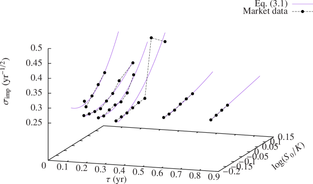
Figure 1: Implied volatilities for Intesa San Paolo: market data (dark points) and parabolic approximation, see Eq. (13).

Table 2. Individual smiles are very well reproduced and for long time to maturities the curves flatten, as expected, while the highest implied kurtosis corresponds to the shortest $\tau$. For $\tau=0.3260$ yr we notice that the volatilities for extreme positive log-moneyness are suspiciously out of scale. We calibrate on the entire data set, but we expect that this large fluctuations will not be reproduced by the models under investigation.

Find optimal $\alpha$, $k$, $m$, and $\rho$ from the time scaling of $\sigma_{\tau}$, $\zeta_{\tau}$ and $\kappa_{\tau}$. The calibration can be done by fitting the values reported in Table 2 with those computed from the models. The scaling of $\sigma_{\tau}$, $\zeta_{\tau}$ and $\kappa_{\tau}$ with $\tau$ is known analytically for the Linear and S2 models, while it can be estimated numerically for ExpOU. For the latter case, we sample $N_{MC}=10^{5}$ paths and we obtain the MC estimators $\sigma_{\tau}^{MC}$, $\zeta_{\tau}^{MC}$, $\kappa_{\tau}^{MC}$ with associated standard errors $\epsilon_{\sigma_{\tau}}^{MC}$, $\epsilon_{\zeta_{\tau}}^{MC}$ and $\epsilon_{\kappa_{\tau}}^{MC}$. The set of optimal values satisfies the equation

$$\alpha^{*},k^{*},m^{*},\rho^{*}=\mathop{\mathrm{argmin}}_{\alpha,k,m>0,~{}\rho\in[-1,1]}\sum_{\tau}\left[\frac{(\sigma_{\tau}^{Mk}-\sigma_{\tau})^{2}}{{\epsilon^{2}_{\sigma_{\tau}}}}+\frac{(\zeta_{\tau}^{Mk}-\zeta_{\tau})^{2}}{{\epsilon^{2}_{\zeta_{\tau}}}}+\frac{(\kappa_{\tau}^{Mk}-\kappa_{\tau})^{2}}{{\epsilon^{2}_{\kappa_{\tau}}}}\right]~{},$$

where $\epsilon^{2}_{\sigma_{\tau}}={\epsilon_{\sigma_{\tau}}^{Mk}}^{2}+{\epsilon_{\sigma_{\tau}}^{MC}}^{2}$, and analogously for $\epsilon^{2}_{\zeta_{\tau}}$ and $\epsilon^{2}_{\kappa_{\tau}}$, the MC error being zero for the Linear and S2 models since their cumulants are known analytically and no MC simulation is required. The optimization problem is solved by means of MINUIT routines [29] and the final results are contained in Table 3. The value of $\beta$ of order $10\%$ from the calibration of the ExpOU dynamics supports the accuracy of the linear approximation, while no statistically significant differences are observed between the Linear and the S2 models.

Optimal parameters for the three models.

Figure 2: Comparison between market implied volatility smiles for Intesa San Paolo and those obtained from the Linear model. Parameters values as in the third row of Table 3, as obtained from the calibration of the Linear model.

Figure 3: Comparison between market implied volatility smiles for Intesa San Paolo and those obtained from the ExpOU and Linear models. Parameters values as in the first row of Table 3, as obtained from the calibration of the ExpOU model.

In Fig. 3.1 we present the smiles for the set of parameters corresponding to the ExpOU calibration and we plot both the curves obtained from MC simulation ($N_{MC}=10^{5}$) of the exponential model and those computed integrating Eq.(LABEL:eq:lewisprice) for the Linear model with the same parameters values (curves corresponding to the linear case have been shifted rightward). In Fig. 4 we plot the PDF of the Linear model against the one for the ExpOU model computed with trapezoidal integration and MC simulation, respectively. Both panels confirm the analysis performed in [12], showing fatter tails and a lower central peak for the histogram of the ExpOU with respect to the PDF of the Linear model.

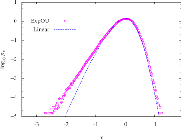
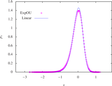
Figure 4: Comparison between $p_{x}(x,\tau|X_{0},Z_{0})$ with $\tau=1$ for the Linear and ExpOU models in log-linear (left panel) and linear (right panel) scales. Parameters values as in the first row of Table 3.

Even though the value $\beta\sim 13\%$ (see Table 3) is at the edge of the regime allowing the linearisation, as far as the volatility smiles obtained from the two models are concerned, we conclude that they are in a good statistical agreement. In Fig. 3.1 a comparison analogous to the one in Fig. 3.1 for the S2 parameters is reported, revealing again the statistical agreement. With respect to Fig. 3.1, the narrower error bars reflect the fact that parameters fitting has been performed exploiting the available analytical information. Actually, the MC simulation involved both in the calibration and the price computation for ExpOU introduces an additional statistical uncertainty.

Figure 5: Comparison between market implied volatility smiles for Intesa San Paolo and those obtained from the S2 and Linear models. Parameters values as in the second row of Table 3, as obtained from the calibration of the S2 model.

4 Conclusions and Perspectives

This paper deals with the problem of option pricing under stochastic volatility and calibration to market smiles. The main focus is on a specific SVM where the dynamics of financial log-returns is driven by linear drift and diffusion coefficients, which we show to be the limit case of the exponential Ornstein-Uhlenbeck and the Stein-Stein models under the low volatility fluctuation regime. The analytical contribution we provide is the exact characterization of the characteristic function of the Linear model under risk neutrality. Following the market practice, we calibrate the model on a sample of implied volatilities by means of the two step calibration procedure detailed in Section 3. In this regard, the knowledge of the analytical expressions of the cumulants substantially reduces the computational effort required to fix the parameters values. For the considered data, we are able to quantitatively asses the capability of the model to reproduce the market volatility smiles, finding a statistically significant agreement with the empirical curves. By means of the same procedure, we also compute the implied volatility values under the ExpOU and S2 models after calibration to evaluate the accuracy of the linear approximation. In both cases, the propagation of the statistical uncertainty results in an error band which clearly reveals that the three models are all in full agreement. In particular, the measured value of $\beta$ for the ExpOU model justifies its linearisation, whose degree of analytical tractability makes it more desirable in view of option pricing.

In this work, we exploited the Greeks to evaluate the statistical uncertainty of the reconstructed volatility smiles; as a future perspective, it would be interesting to analyze the sensitivity with respect to movements of market volatility curves, which is what is done in financial practice by traders to hedge option positions. We also aim at applying the Linear model considered here in the context of market risk measures, like Value-at-Risk and Expected Shortfall, exploiting the knowledge of the analytical CF following the guidelines traced by [30]. For risk management purposes, it would be interesting to analytically characterize the PDF tails. Indeed, the numerical convergence of the integral in Eq. (LABEL:eq:lewisprice) excludes a power law decay, but an explicit analytical result such as for the Heston [31] and the ExpOU models [32] discerning between exponential, Gaussian or different scalings is still lacking.

Acknowledgments

We wish to acknowledge the anonymous referee for fruitful comments and for giving us the opportunity, through his criticism, of improving the paper in several respects. We also thank Enrico Melchioni, Guido Montagna, Oreste Nicrosini, Andrea Pallavicini and Fulvio Piccinini for their suggestions. We are grateful to FMR Consulting for having provided the market data.

Appendix A Linear model cumulants

In the following we report the analytical expressions of the cumulants of the Linear model.

$$k_{1,\tau}=-\frac{m^{2}}{2}\int_{0}^{\tau}\mathcal{M}(\tau^{\prime})\mathrm{d}\tau^{\prime}+\frac{m^{2}}{\alpha}(Z_{0}-1)(e^{-\alpha\tau}-1)-\frac{m^{2}}{2\alpha}\alpha\tau+X_{0},$$

$$k_{2,\tau}=\frac{1}{4}\frac{m^{2}}{\alpha} \bigg{\{}-2\left(\frac{km}{\alpha}\right)^{2}\left[e^{-2\alpha\tau}-4e^{-\alpha\tau}-2\alpha\tau+3\right]+\frac{k^{2}}{\alpha}\left[e^{-2\alpha\tau}+2\alpha\tau-1\right]$$

$$-2(Z_{0}-1)^{2}\left[e^{-2\alpha\tau}-1\right]-8(Z_{0}-1)\left[e^{-\alpha\tau}-1\right]+4\alpha\tau\bigg{\}}$$

$$+2~{}\frac{km^{3}}{\alpha^{2}}\rho~{} \bigg{\{}(Z_{0}-1)\left[e^{-\alpha\tau}+\alpha\tau e^{-\alpha\tau}-1\right]-\left[e^{-\alpha\tau}+\alpha\tau-1\right]\bigg{\}},$$

$$k_{3,\tau}=\frac{3}{2}\frac{k^{2}m^{3}}{\alpha^{3}} \bigg{\{}(Z_{0}-1)\left[e^{-3\alpha\tau}-2e^{-2\alpha\tau}+e^{-\alpha\tau}(3+2\alpha\tau)-2\right]+2\left[e^{-2\alpha\tau}-4e^{-\alpha\tau}-2\alpha\tau+3\right]\bigg{\}}$$

$$+\frac{3}{2}\frac{km^{3}}{\alpha^{2}}\rho~{} \bigg{\{}\left(\frac{km}{\alpha}\right)^{2}\left[-e^{-2\alpha\tau}(3+2\alpha\tau)+4e^{-\alpha\tau}(3+\alpha\tau)+4\alpha\tau-9\right]+\frac{k^{2}}{\alpha}\left[e^{-2\alpha\tau}(1+\alpha\tau)+\alpha\tau-1\right]$$

$$- (Z_{0}-1)^{2}\left[e^{-2\alpha\tau}(1+2\alpha\tau)-1\right]+2(Z_{0}-1)\left[e^{-2\alpha\tau}-2e^{-\alpha\tau}(2+\alpha\tau)+3\right]+4\left[e^{-\alpha\tau}+\alpha\tau-1\right]\bigg{\}}$$

$$+3~{}\frac{k^{2}m^{4}}{\alpha^{3}}\rho^{2} \bigg{\{}(Z_{0}-1)\left[e^{-\alpha\tau}(2+2\alpha\tau+\alpha^{2}\tau^{2})-2\right]-2\left[e^{-\alpha\tau}(2+\alpha\tau)+\alpha\tau-2\right]\bigg{\}},$$

$$k_{4,\tau}=3~{}\frac{k^{2}m^{4}}{\alpha^{3}} \bigg{\{}\frac{1}{2}\left(\frac{km}{\alpha}\right)^{2}\left[-e^{-4\alpha\tau}+4e^{-3\alpha\tau}-4e^{-2\alpha\tau}(3+\alpha\tau)+4e^{-\alpha\tau}(7+2\alpha\tau)+8\alpha\tau-19\right]$$

$$+\frac{k^{2}}{8\alpha}\left[e^{-4\alpha\tau}+4e^{-2\alpha\tau}(1+2\alpha\tau)+4\alpha\tau-5\right]-\frac{1}{2}(Z_{0}-1)^{2}\left[e^{-4\alpha\tau}+4\alpha\tau e^{-2\alpha\tau}-1\right]$$

$$+2(Z_{0}-1)\left[-e^{-3\alpha\tau}+2e^{-2\alpha\tau}-e^{-\alpha\tau}(3+2\alpha\tau)+2\right]+2\left[-e^{-2\alpha\tau}+4e^{-\alpha\tau}+2\alpha\tau-3\right]\bigg{\}}$$

$$+6~{}\frac{k^{3}m^{5}}{\alpha^{4}}\rho~{} \bigg{\{}(Z_{0}-1)\left[3e^{-3\alpha\tau}(1+\alpha\tau)-2e^{-2\alpha\tau}(3+2\alpha\tau)+e^{-\alpha\tau}(9+7\alpha\tau+2\alpha^{2}\tau^{2})-6\right]$$

$$+\left[-e^{-3\alpha\tau}+2e^{-2\alpha\tau}(5+2\alpha\tau)-e^{-\alpha\tau}(35+10\alpha\tau)-12\alpha\tau+26\right]\bigg{\}}$$

$$+3~{}\frac{k^{2}m^{4}}{\alpha^{3}}\rho^{2} \bigg{\{}4\left(\frac{km}{\alpha}\right)^{2}\left[-e^{-2\alpha\tau}(3+3\alpha\tau+\alpha^{2}\tau^{2})+e^{-\alpha\tau}(12+6\alpha\tau+\alpha^{2}\tau^{2})+3\alpha\tau-9\right]$$

$$+\frac{k^{2}}{\alpha}\left[e^{-2\alpha\tau}(3+4\alpha\tau+2\alpha^{2}\tau^{2})+2\alpha\tau-3\right]-2(Z_{0}-1)^{2}\left[e^{-2\alpha\tau}(1+2\alpha\tau+2\alpha^{2}\tau^{2})-1\right]$$

$$+4(Z_{0}-1)\left[2e^{-2\alpha\tau}(1+\alpha\tau)-e^{-\alpha\tau}(6+4\alpha\tau+\alpha^{2}\tau^{2})+4\right]$$

$$-2\left[e^{-2\alpha\tau}-4e^{-\alpha\tau}(3+\alpha\tau)-6\alpha\tau+11\right]\bigg{\}}$$

$$4~{}\frac{k^{3}m^{5}}{\alpha^{4}}\rho^{3} \bigg{\{}(Z_{0}-1)\left[e^{-\alpha\tau}(6+6\alpha\tau+3\alpha^{2}\tau^{2}+\alpha^{3}\tau^{3})-6\right]-3\left[e^{-\alpha\tau}(6+4\alpha\tau+\alpha^{2}\tau^{2})+2\alpha\tau-6\right]\bigg{\}}~{}.$$

From the asymptotic expansions $k_{2,\tau}\sim-m^{2}(2Z_{0}-1)\tau/2$, $k_{3,\tau}\sim 3km^{3}Z_{0}^{2}\rho\tau^{2}$, and $k_{4,\tau}\sim 4k^{2}m^{4}(1+2\rho^{2})Z_{0}^{2}\tau^{3}$ when $\tau\rightarrow 0^{+}$, we can infer the leading behaviour of skewness and kurtosis at the origin

$$\zeta_{\tau}\sim 3\frac{k\rho}{Z_{0}}\sqrt{\tau}\quad\text{and}\quad\kappa_{\tau}\sim 4\frac{k^{2}(1+2\rho^{2})}{Z_{0}^{2}}\tau.$$

References

- [1] F. Black and M. Scholes, The pricing of options and corporate liabilities, J. Polit. Economy 81 (1973) 637.
- [2] R. Merton, Theory of rational option pricing, Bell J. Econ. Management Sci. 4 (1973) 141.
- [3] S. Heston, A closed-form solution for options with stochastic volatility with applications to bond and currency options, Rev. Finan. Stud. 6 (1993) 327.
- [4] E.M. Stein and J.C. Stein, Stock price distributions with stochastic volatility: An analytic approach, Rev. Finan. Stud. 4 (1991) 727.
- [5] R. Schöbel and J. Zhu, Stochastic volatility with an Ornstein Uhlenbeck process: An extension, Europ. Finance Rev. 4 (1999) 23.
- [6] J. Hull and A. White, The pricing of options on asset with stochastic volatilities, J. Finance 42 (1987) 281.
- [7] L. Scott, Option pricing when the variance changes randomly: Theory, estimators and applications, J. Finan. Quant. Anal. 22 (1987) 419.
- [8] S. Miccichè, G. Bonanno, F. Lillo and R. N. Mantegna, Volatility in financial markets: Stochastic models and empirical results. Physica A 314 (2002) 756.
- [9] A. Lipton and A. Seppt, Stochastic volatility models and Kelvin waves, J. Phys. A 41 (2008) 344012.
- [10] S. Mitra, A review of volatility and option pricing. Preprint available at: http://arxiv.org/pdf/0904.1292.
- [11] J. Masoliver and J. Perelló, Multiple time scales and the exponential Ornstein-Uhlenbeck stochastic volatility model, Quant. Finance 6 (2006) 423.
- [12] G. Bormetti, V. Cazzola, G. Montagna and O. Nicrosini, The probability distribution of returns in the exponential Ornstein - Uhlenbeck model, J. Stat. Mech. (2008) P11013.
- [13] P. Carr and D.B. Madan, Option valuation using the Fast Fourier Transform, J. Comp. Finance 2 (1999) 61.
- [14] A. L. Lewis, A simple option formula for general jump - diffusion and other exponential Lévy processes, Envision Financial Systems and OptionCity.net Technical Report (2001). Available at http://www.optioncity.net.
- [15] A. Lipton, Mathematical Methods For Foreign Exchange: A Financial Engineer’s Approach, World Scientific Publishing (2001).
- [16] R. Lord and C. Kahl, Complex logarithms in Heston-like models. Available at http://ssrn.com/abstract=1105998.
- [17] J. Perelló, Market memory and fat tail consequences in option pricing on the expOU stochastic volatility, Physica A 382 (2007) 213.
- [18] J. Perelló, R. Sircar and J. Masoliver, Option pricing under stochastic volatility: The exponential Ornstein-Uhlenbeck model, J. Stat. Mech. (2008) P06010.
- [19] J. P. Fouque, G. Papanicolau and K. R. Sircar, Derivatives in financial markets with stochastic volatility, Cambridge University Press (2006).
- [20] J. Masoliver and J. Perelló, A correlated stochastic volatility model measuring leverage and other stylized facts, Int. J. Theoretical Appl. Finance 5 (2002) 541.
- [21] G. ’t Hooft and M. Veltman, Scalar one-loop integrals, Nucl. Phys. B 153 (1979) 365.
- [22] S. Mikhailov and U. Nögel, Heston’s stochastic volatility model: Implementation, calibration and some extensions, in The Best of Wilmott 1: Incorporating the Quantitative Finance Review, P. Wilmott (ed.), John Wiley and Sons (2004).
- [23] S. Galluccio and Y. Le Cam, Implied calibration of stochastic volatility jump diffusion models, (2005). Available at http://129.3.20.41/eps/fin/papers/0510/0510028.pdf.
- [24] M. Forde, A. Jaquier and A. Mijatovic, Asymptotic formulae for implied volatility in the Heston model, arXiv0911.2992 (2009).
- [25] D. K. Backus, S. Foresi and L. Wu, Accounting for biases in Black-Scholes, Technical report (2004). Available at SSRN: http://ssrn.com/abstract=585623.
- [26] J. P. Bouchaud and M. Potters, Theory of Financial Risk and Derivative Pricing: From Statistical Physics to Risk Management, Cambridge University Press (2000).
- [27] S. Ciliberti, J. P. Bouchaud and M. Potters, Smile dynamics: A theory of the implied leverage effect. Preprint available at http://lanl.arxiv.org/abs/0809.3375.
- [28] W. H. Press, B. P. Flannery, S. A. Teukolsky and W. T. Vetterling, Numerical recipes – The art of scientific computing, Cambridge University Press, New York (1989).
- [29] F. James, MINUIT Function Minimization and Error Analysis Reference Manual, CERN Geneva, Switzerland (1998). Available at: http://wwwasdoc.web.cern.ch/wwwasdoc/minuit/minmain.html.
- [30] G. Bormetti, V. Cazzola, G. Livan, G. Montagna and O. Nicrosini, A generalized Fourier transform approach to risk measures, J. Stat. Mech. (2010) P01005.
- [31] A. A. Dragŭlescu and V. M. Yakovenko, Probability distribution of returns in the Heston model with stochastic volatility, Quant. Finance 2 (2002) 443.
- [32] B. Jourdain, Loss of martingality in asset price models with lognormal stochastic volatility, Preprint CERMICS 2004-267 available at http://cermics.enpc.fr/ jourdain/publications.html.