Low-order models of 2D fluid flow in annulus

The two-dimensional flow of viscous incompressible fluid in the domain between two concentric circles is investigated numerically. To solve the problem, the low-order Galerkin models are used. When the inner circle rotates fast enough, two axially asymmetric flow regimes are observed. Both regimes are the stationary flows precessing in azimuthal direction. First flow represents the region of concentrated vorticity. Another flow is the jet-like structure similar to one discovered earlier in experiments [1, 2].

Introduction

The interest to the problem considered is stimulated by the strange flow regimes induced in the thin fluid layer by the rotating cylinder, experimentally discovered by V. A. Vladimirov [1, 2] in 1994. The flow in a thin annular gap restricted in axial direction by rigid walls was considered. When the inner cylinder rotates fast enough, axially asymmetric, slow-precessing, stable jet-like pattern appears. These jets represent the sectors with the strong radial outflow which precesses in azimuthal direction.

The flow regimes observed in experiments are not deeply investigated and the mechanism of their onset is not clear. The flow observed is not the Moffatt vortex that appears in the domain with corners [3]. It is not the Hammel flow with the azimuthal jets, investigated and classified by M. A. Goldshtik, V. N. Shtern et al. (see for example [4, 5, 6] where the flow regimes without the inner cylinder but with the source are considered). It is not the spiral structure described in works by M. V. Nezlin and E. N. Snezhkin [7, 8] that appears in the thin layer of rotating fluid with a free surface with differentially rotating parabolic-shape bottom. We notice that in spite of visual similarity with regimes from [7, 8], flows in [1, 2] are totally different. In [7, 8] the reason for the spiral structure onset is the parabolic bottom profile that models the gravity field in the radial direction, so that the phenomenon could be described with the use of shallow water theory. In other words the jet-like structures in [7, 8] are similar to waves on the free surface. Here it is worth mentioning works by V. Yu. Liapidevsky (see for example [9]) on the two-dimensional vortical shallow water flows in a gap between two rigid boundaries.

There is a number of works on the similar problems. These works are mainly devoted to study the axially symmetric regimes in the Couette-Taylor flow between short cylinders. These problems were intensively investigated numerically after T. B. Benjamin and T. Mullin [10]. The axially symmetric flows in the annular gap with comparable radial and axial sizes, governed by the two-dimensional Navier-Stokes equations were studied with the help of the finite-difference methods (particularly the methods of markers and cells, and their modifications) and of the Galerkin method (see for example [10, 11, 12, 13, 14]). The base axially symmetric flow regime in the domain with two rigid end-walls represents two Taylor vortices. The bifurcation of this flow to the regime with one major vortex and one minor vortex is described.

In works [15, 16, 17, 18] the asymptotic model describing the base axially symmetric regime in the thin in axial direction annular domain between two cylinders is constructed and compared with experiment. This asymptotic model describes two Taylor vortices in the case of rigid end-walls and one Taylor vortex in the case when one of the end-walls is the non-deformable free surface. Particularly, the analytic formula has been obtained for the azimuthal velocity (it was earlier defined numerically in [11, 12, 13, 14]). The azimuthal velocity calculated with the help of this analytic formula is in a good agreement with the experimental data [15, 16, 17, 18].

In the work presented we attempt to model some of the experimental results from [1, 2] with the use of the low-order Galerkin model, applied to the viscous flow in the two-dimensional annular strip. When the base flow similar to the Couette flow loses stability for the low-order model, the stationary asymmetric flow (the soliton-like vortex) appears. This vortex slowly precesses in the azimuthal direction. Furthermore, numerical experiments with the low-order models allowed to discover another axially asymmetric stationary flow regime: slow precessing in the azimuthal direction jet-like structure. This axially asymmetric solution (apart from the first one) does not bifurcate from the base flow but appears ’from the sky-blue’. The jet-like regimes appear to be similar to ones observed in experiments presented in [1, 2]. It is rather surprising because, according to [1, 2, 15, 16, 17, 18], the jet-like flows observed in the narrow (in axial direction) gap are substantially three-dimensional. Another surprise is that the Reynolds numbers for which asymmetric structures appear are of the same order as in the experiments. Comparison of the other parameters is impossible since the numerically solved problem is two-dimensional while the experimental facility is essentially three-dimensional.

The certain uneasiness is caused by dependence of the results of numerical modeling on the number of radial basis functions for Galerkin model. With the increase of the number of this functions, increase of the critical Reynolds numbers is observed (note that the results weakly depend on the number of azimuthal basis functions). In other words, results obtained (existence of the precessing stationary flows in the form of the soliton-like jet or the soliton-like vortex) could be specific for the low-order Galerkin models only, while the base flow could be stable for the high-order models. However, good qualitative agreement with the experiments described in [1, 2] make us hope that the low-order models are useful to improve the understanding of the mechanism of jet-like structures onset in the gaps narrow in the axial direction.

1 Basic equations

Let the annular strip domain bounded by the circles of radii $r_{1}$ и $r_{2}$ ($r_{1}<r_{2}$) is filled by the viscous incompressible fluid. The inner boundary $r=r_{1}$ is rotating with the constant azimuthal velocity $\Omega$, and the outer boundary $r=r_{2}$ is fixed. The Navier-Stokes equations in the polar coordinates $(r,\theta)$ in the dimensionless form are:

$$u_{t}+uu_{r}+\frac{1}{r}\,\,vu_{\theta}-\frac{v^{2}}{r}=-p_{r}+\operatorname{Re}^{-1}\left(\Delta u-\frac{u}{r^{2}}-\frac{2}{r^{2}}\,\,v_{\theta}\right),$$

$$v_{t}+uv_{r}+\frac{1}{r}\,\,vv_{\theta}+\frac{uv}{r}=-\frac{1}{r}\,\,p_{\theta}+\operatorname{Re}^{-1}\left(\Delta v-\frac{v}{r^{2}}+\frac{2}{r^{2}}\,\,u_{\theta}\right),$$ (1.1)

$$(ru)_{r}+v_{\theta}=0,$$

$$\Delta(\quad)=(\quad)_{rr}+\frac{1}{r}\,\,(\quad)_{r}+\frac{1}{r^{2}}\,\,(\quad)_{\theta\theta}.$$

Here $u$ is the radial velocity, $v$ is the azimuthal velocity, $p$ is the pressure, $\operatorname{Re}$ is the Reynolds number.

Boundary conditions at $r=1$ and $r=b$ have the form:

$$\left.u\right|_{r=1}=0,\quad\left.v\right|_{r=1}=1,\quad\left.u\right|_{r=b}=0,\quad\left.v\right|_{r=b}=0.$$ (1.2)

Dimensionless variables $t$, $r$, $u$, $v$, $p$ correspond to dimensional variables $t^{\prime}$, $r^{\prime}$, $u^{\prime}$, $v^{\prime}$, $p^{\prime}$:

$$t^{\prime}=\frac{t}{\Omega},\quad r^{\prime}=rr_{1},\quad(u^{\prime},v^{\prime})=\Omega r_{1}(u,v),\quad p^{\prime}=p\rho\Omega^{2}r_{1}^{2},$$

$$\operatorname{Re}=\frac{\Omega r_{1}^{2}}{\nu},\quad\varepsilon=\operatorname{Re}^{-1},\quad b=\frac{r_{2}}{r_{1}}.$$ (1.3)

where $\nu$ is the kinematic viscosity, $r_{1}$ is the radius of the inner circle, $r_{2}$ is the radius of the outer circle, $\Omega$ is the azimuthal velocity of the inner circle rotation, $\rho$ is the constant fluid density.

The problem (1.1)–(1.2) has the stationary axially symmetric solution (Couette flow):

$$u=0,\quad v=V_{0}(r),\quad V_{0}(r)=\frac{\alpha}{r}+\beta r,\quad\alpha=\frac{b^{2}}{b^{2}-1},\quad\beta=-\frac{1}{b^{2}-1}.$$ (1.4)

Let $\Psi(t,r,\theta)$ be a stream function and $\psi(t,r,\theta)$ be a perturbation of the stream function:

$$u=-\frac{1}{r}\psi_{\theta}=-\frac{1}{r}\Psi_{\theta},\quad v=\psi_{r}+V_{0}=\Psi_{r}.$$ (1.5)

If we substitute (1.5) to (1.1)–(1.2), we obtain:

$$\Delta\psi_{t}+\frac{1}{r}\bigl{(}\psi_{r}(\Delta\psi)_{\theta}-\psi_{\theta}(\Delta\psi)_{r}\bigr{)}=\varepsilon\Delta^{2}\psi-\frac{V_{0}}{r}(\Delta\psi)_{\theta},$$ (1.6)

$$\left.\psi\right|_{r=1}=0,\quad\left.\psi_{r}\right|_{r=1}=0,\quad\left.\psi\right|_{r=b}=0,\quad\left.\psi_{r}\right|_{r=b}=0.\quad$$ (1.7)

2 Galerkin approximations

To obtain the approximate solution of the problem (1.6)–(1.7), Galerkin method is used. We approximate the stream function perturbation $\psi$ as follows:

$$\psi=2\sum_{m=1}^{L}\sum_{n=1}^{N}\left\{(x_{mn}(t)\cos(n\theta)-y_{mn}(t)\sin(n\theta)\right\}f_{mn}(r).$$ (2.1)

Here, the functions $f_{mn}(r)$ satisfy the boundary conditions:

$$f_{mn}(1)=0,\quad f^{\prime}_{mn}(1)=0,\quad f_{mn}(b)=0,\quad f^{\prime}_{mn}(b)=0,\quad$$ (2.2)

The standard Galerkin procedure reduces the problem (1.6)–(1.7) to the system of the ordinary differential equations for Galerkin coefficients $x_{mn}(t)$, $y_{mn}(t)$. We also assume that the functions $f_{mn}(r)$ satisfy the following conditions:

$$\int\limits_{1}^{b}f_{mn}(r)\Delta_{n}f_{jn}(r)r\,dr=-\delta_{jm}$$ (2.3)

$$\Delta_{n}(\,\,)=(\ )_{rr}+\frac{1}{r}(\ )_{r}-\frac{n^{2}}{r^{2}}(\ ).$$ (2.4)

In the work [19] the two-dimensional flow in the annular strip (driven by the azimuthal force changing the sign with radius) is studied. Analogously to the work [19] the functions $f_{mn}(r)$ for fixed $n$ are taken as the eigenfunctions of the following boundary value problem:

$$\Delta_{n}^{2}f+h^{2}\Delta_{n}f=0,$$ (2.5)

$$f(1)=0,\quad f^{\prime}(1)=0,\quad f(b)=0,\quad f^{\prime}(b)=0$$ (2.6)

Calculation of the eigenvalues $h_{mn}$ for the problem (2.5)–(2.6) and of the corresponding eigenfunctions $f_{mn}(r)$ is a tiresome procedure. That is why we also use the polynomial basis to construct functions $f_{mn}(r)$.

To determine Galerkin coefficients $x_{mn}(t)$, $y_{mn}(t)$, the following system of the ordinary differential equations is obtained:

$$\frac{dx_{mn}}{dt}=-\varepsilon\sum_{j=1}^{L}\delta_{mjn}x_{jn}-\sum_{j=1}^{L}\gamma_{mjn}y_{jn}-\sum_{j=1}^{L}\sum_{p=1}^{L}\sum_{k=1}^{N}\sum_{q=1}^{N}(\alpha_{kqn}x_{jk}y_{pq}-\beta_{kqn}y_{jk}x_{pq})K_{jkpqmn},$$ (2.7)

$$\frac{dy_{mn}}{dt}=-\varepsilon\sum_{j=1}^{L}\delta_{mjn}y_{jn}+\sum_{j=1}^{L}\gamma_{mjn}x_{jn}+\sum_{j=1}^{L}\sum_{p=1}^{L}\sum_{k=1}^{N}\sum_{q=1}^{N}(\beta_{qnk}x_{jk}x_{pq}-\beta_{knq}y_{jk}y_{pq})K_{jkpqmn}.$$

Here

$$\alpha_{kqn}=1,\ \text{if\ }\ n=|k-q|\ \ \text{or\ }\ n=k+q;\ \ \alpha_{kqn}=0,\ \text{otherwise};$$

$$\beta_{kqn}=1,\ \text{if\ }\ n=|k-q|;\ \ \beta_{kqn}=-1,\ \text{if\ }\ n=k+q;\ \ \beta_{kqn}=0,\ \text{otherwise}.$$

The coefficients $\delta_{mjn}$, $\gamma_{mjn}$ and $K_{jkpqmn}$ are defined by the following relations:

$$\delta_{mjn}=\int\limits_{1}^{b}f_{mn}\Delta_{n}g_{jn}r\,dr,\quad\gamma_{mjn}=n\int\limits_{1}^{b}V_{0}f_{mn}g_{jn}\,dr,$$ (2.8)

$$K_{jkpqmn}=q\int\limits_{1}^{b}(f^{\prime}_{jk}g_{pq}-g^{\prime}_{jk}f_{pq})f_{mn}\,dr,\quad g_{jn}=\Delta_{n}f_{jn}.$$

3 Numerical experiments

Solutions of the system of equations (2.7) depend on the two dimensionless parameters: the Reynolds number $\operatorname{Re}$ (or $\varepsilon=\operatorname{Re}^{-1}$) and on the ratio of the outer and inner radii $b$. Note that the parameter $\varepsilon$ is included to the system (2.7) explicitly whereas the coefficients $\delta_{mjn}$, $\gamma_{mjn}$ и $K_{jkpqmn}$ depend on the parameter $b$.

3.1 Basis functions

Two sets of the basis functions are in use: the set of solutions of the problem (2.5)–(2.6), and the linear combinations of the polynomials $P_{m}(r)=(r-1)^{2}(b-r)^{2}r^{m-1}$ which satisfy the conditions (2.2)–(2.4).

Solutions of the problem (2.5)–(2.6) have the form [19]:

$$f_{mn}(r)=\bigl{[}A_{mn}J_{n}(\rho)+B_{mn}Y_{n}(\rho)+C_{mn}\rho^{n}+D_{mn}\rho^{-n}\bigr{]}/h_{mn}^{2},\,\,\rho=h_{mn}r$$

where $J_{n}$ is the Bessel function of the first kind, $Y_{n}$ is the Neumann function.

The eigenvalues $h_{mn}$ and coefficients $A_{mn}$, $B_{mn}$, $C_{mn}$, $D_{mn}$ are defined by the boundary conditions:

$$f_{mn}(1)=0,\quad f^{\prime}_{mn}(1)=0,\quad f_{mn}(b)=0,\quad f^{\prime}_{mn}(b)=0$$ (3.1)

Values $h_{mn}$, ($m=1,2,\dots,L$) are the roots of the determinant of the system (3.1). The nontrivial solution $(A_{mn},B_{mn},C_{mnl},D_{mn})$ of the system (3.1) must satisfy the condition (2.3). The function $g_{mn}$ has the form:

$$g_{mn}=\Delta_{n}f_{mn}=A_{mn}J_{n}(\rho)+B_{mn}Y_{n}(\rho).$$

The system of functions $P_{m}(r)=(r-1)^{2}(b-r)^{2}r^{m-1}$ is used to construct the polynomial basis. Functions $f_{mn}(r)$ for fixed $n$ are constructed with the help of Gramm-Shchmidt orthogonalization with the scalar product:

$$(u,v)=-\int_{1}^{b}u(r)\Delta_{n}v(r)r\,dr,\quad(f_{mn},f_{mn})=1.$$

Chosen sets of basis functions are almost identical. Indeed, as the numerical experiment showed, properties of the solution of (1.6)–(1.7) obtained by Galerkin method weakly depend on the choice of system of the basis functions $f_{mn}(r)$. The number $L$ of the radial basis functions is chosen to be 2 or 3, and the number $N$ of the azimuthal basis functions is not more then 9.

3.2 Dependence of the critical Reynolds numbers on the number of basis functions

Equations (2.7) have the solution which corresponds to the base regime (Couette flow). For the small Reynolds numbers this flow is stable, however, it can become unstable when the Reynolds number increases. The neutral curve $\operatorname{Re}=\operatorname{Re}_{0}(b)$ for $N=9$, $L=3$ is shown in Fig. 1 (left). The neutral curve corresponds to the oscillatory instability with the azimuthal wave number $n=1$. Neutral curves with the azimuthal wave numbers $n=2,\,3$ have similar form.

Figure 1: Left: the neutral curve $\operatorname{Re}=\operatorname{Re}_{0}(b)$ of the Couette flow instability, corresponding to the azimuthal wave number $n=1$ ($L=3$, $N=9$, polynomial basis). Right: dependence of the critical Reynolds numbers on the number of basis functions $L$ at $b=5$. Continuous line corresponds to computation with polynomial basis; circles correspond to basis composed of the eigenfunctions of (2.5)–(2.6); azimuthal wave number $n=1$.

When the parameter $b$ is fixed, the critical Reynolds numbers $\operatorname{Re}_{0}(b)$ are strongly dependent on $L$ (the number of radial basis functions). Numerical investigation of the linear stability of the solution $x_{mn}=0$, $y_{mn}=0$ of equations (2.7) shows that the critical Reynolds numbers are monotonously increasing with the increase of $L$ when $L\geqslant 6$. Results of calculation at $b=5$ are presented in Fig. 1 (right). Continuous line corresponds to the polynomial basis, and circles represent basis composed from the eigenfunctions of the problem (2.5)–(2.6).

3.3 Flow regimes

Two different stable stationary regimes (traveling waves) are found apart from the base Couette flow in numerical experiments performed. Galerkin coefficients $x_{mn}(t)$ and $y_{mn}(t)$ are periodic functions of time $t$, while the amplitudes $d_{mn}=(x_{mn}^{2}+y_{mn}^{2})^{1/2}$ are constant for these regimes. One of them appears as a result of instability of the base Couette flow. Nature of the second regime is still not clear. Both flows have a number of typical features that are independent of the outer radius $b$, the choice of the basis functions $f_{mn}(r)$ and the number of these functions $L$ (for small enough $L$) provided that a number of the azimuthal basis functions is chosen to be large enough.

Figure 2: Dependence of the amplitude $d_{11}$ on the Reynolds number: continuous line corresponds to regime with precessing vortex; circles correspond to regime with the jet. Left picture correspond to $b=5$, right picture corresponds to $b=7$, polynomial basis is used in both cases. Regime J is stable at $110\,<\operatorname{Re}<\,290$ for $b=7$, and at $175\,<\operatorname{Re}<\,480$ for $b=5$.

In the wide interval of parameters regimes observed are stable. The onset of one or another of these regimes depends on the initial conditions. One regime is the stationary flow with the single precessing vortex spot. We call it ’regime V’. Main feature of the second flow regime is the region of intensive flow in the form of the radial jet, precessing in the azimuthal direction. We call it ’regime J’.

In the models constructed with the use of polynomial basis by $r$, the system loses stability smoothly in the sense that the periodical motion branches to the supercritical area $\operatorname{Re}>\operatorname{Re}_{0}$ and is stable. If we use the basis composed from the eigenfunctions of the problem (2.5)–(2.6), we observe the rough loss of stability: the unstable limiting cycle branches to the subcritical area.

Figure 3: Dependence of precession speed on the Reynolds number: upper points correspond to regime with precessing vortex, lower points correspond to regime with the jet. Left picture corresponds to $b=5$, right picture corresponds to $b=7$. Polynomial basis is used in both cases.

We emphasize again that there is a certain range of parameters where both stationary flow regimes are stable. The onset of one or another flow regime depends on initial conditions. Regime V typically appears when the initial values of $|\,\bf{v}|$ are small. Regime J is usually observed when the initial values of $\,|\bf{v}|$ are large. Note that the values of $\,d_{mn}$ that correspond to regime J are significantly larger than ones for the flow of V type. The amplitude curves $\,d_{11}=d_{11}(\operatorname{Re})$ are presented in Fig. 2. Note that regime V branches from the base Couette flow whereas regime J appears ’from the sky-blue’. When the Reynolds number increases, the oscillatory instability of flow regime J is observed.

Another characteristic of the flow regimes V and J is the precession speed in the azimuthal direction $w\,=\,\omega/(2\pi)$. Dependence of precession speed on the Reynolds number for two values of $b$ is presented in Fig. 3.

3.4 Flow with a precessing vortex (regime V)

One of the flows observed in numerical experiments is the regime V: periodic flow of the type of a traveling wave with the single vortex that slowly precesses in the azimuthal direction (the direction of the vortex precession coincides with the direction of the inner circle rotation). Onset of this regime is linked to the loss of stability of the base Couette flow. Regime V appears for both sets of basis functions: a set of the eigenfunctions of the problem (2.5)–(2.6) and a set of the polynomials. Typical results of numerical experiment for the flow of the type V are presented in Figs. 4–8. Computation is performed at $L=3$, $N=9$, basis composed of the eigenfunctions of (2.5)–(2.6) is used.

1 2 3 4

Figure 4: Regime V, streamlines (1, 2) and level lines of the stream function perturbation $\psi(r,\theta)$ (3, 4); 1 and 3 correspond to $b=5$, $\operatorname{Re}=320$; 2 and 4 correspond to $b=7$, $\operatorname{Re}=200$.

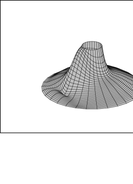
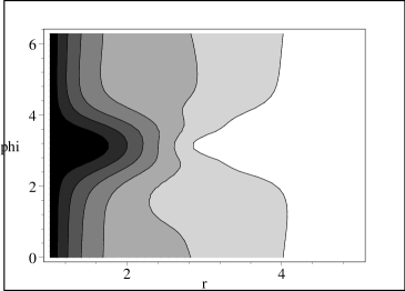
Figure 5: Regime V, $b=5$, $\operatorname{Re}=320$. Left: graph of the absolute velocity $|{\bf{v}}(r,\theta)|$. Right: contour plot of the absolute velocity.

The streamlines and the level lines of the stream function perturbation are plotted in Fig. 4 (location of the soliton-like vortex is clearly visible). Graph of the absolute velocity $|{\bf{v}}(r,\theta)|$ for the flow with the single vortex (regime V) is exposed in Fig. 5 (left). Contour plot of the absolute velocity in the rectangle $r\in[1,b]$, $\theta\in[0,2\pi]$ is shown in Fig. 5 (right). Regions of the different flow intensity are painted with different colors. The value $|\bf{v}|$ is taken as the measure of the flow intensity. The highest flow intensity is observed in the area close to the inner boundary (black color). Note that the values of fluid velocity at the inner and outer boundaries are $|{\bf{v}}|=1$ and $|{\bf{v}}|=0$ correspondingly, and $|{\bf{v}}|=k/7$ $(k=1,2,...,6)$ for level lines in Fig.5 (right). The contour plots of radial velocity $u(r,\theta)$ and azimuthal velocity $v(r,\theta)$ are presented in Fig. 6.

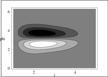
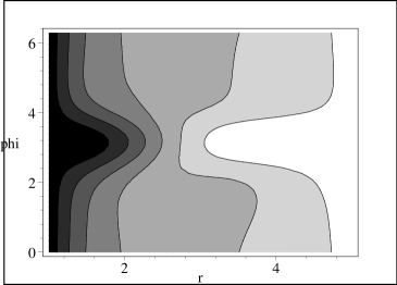
Figure 6: Contour plots of the radial and azimuthal velocity $u(r,\theta)$, $v(r,\theta)$. Flow with precessing vortex; $b=5$, $\operatorname{Re}=320$

Figure 7: Dependence of radial velocity $u(r,\theta)$ and of azimuthal velocity $v(r,\theta)$ on $\theta$ at $r=1+(3k-1)(b-1)/20$, where $k$ is the number of the line. Flow with precessing vortex.

Figure 8: Dependence of vorticity $\Delta\psi(r,\theta)$ and of stream function perturbation $\psi(r,\theta)$ on $\theta$ at $r=1+(3k-1)(b-1)/20$, where $k$ is the number of the line. Flow with precessing vortex.

In Figs. 7–8 radial and azimuthal velocity profiles, vorticity profiles, and stream function perturbation profiles in the cross-sections $r=const$ are presented. Note that zeros of the radial velocity $u(r,\theta)$ almost coincide with the extreme points of the azimuthal velocity $v(r,\theta)$, and zeros of $\Delta\psi(r,\theta)$ almost coincide with zeros of $\psi(r,\theta)$. Extreme points of $\Delta\psi(r,\theta)$ and extreme points of $\psi(r,\theta)$ also almost coincide.

3.5 Flow with a precessing jet (regime J)

Apart from the regime with precessing vortex, another type of stationary flow is observed in numerical experiments. It is the slowly precessing in azimuthal direction stationary structure, whose main feature is existence of the jet-like area of intensive fluid motion.

Results of numerical experiments for regime J are presented in Figs. 9–14. The streamlines and the level lines of the stream function perturbation are plotted in Fig. 9. There is also the precessing vortex, but its shape is more complicated than that for the regime V. The vortex is stretched in the azimuthal direction.

1 2 3 4

Figure 9: Regime J, streamlines (1, 2) and level lines of the stream function perturbation $\psi(r,\theta)$ (3, 4); 1 and 3 correspond to $b=5$, $\operatorname{Re}=320$; 2 and 4 correspond to $b=7$, $\operatorname{Re}=200$. Basis composed of the eigenfunctions of (2.5)–(2.6) is used in both cases.

Graph of the absolute velocity $|{\bf{v}}(r,\theta)|$ for the flow with precessing jet (regime J) and contour plot of the absolute velocity in the rectangle $r\in[1,b]$, $\theta\in[0,2\pi]$ are shown in Fig. 10 (as before, $|\bf{v}|$ is taken as the measure of the flow intensity). The most intensive flow is observed in the certain region close to the inner boundary. Comparison with Fig. 5 shows that the boundary layer near the inner boundary have qualitatively different form for regimes V and J.

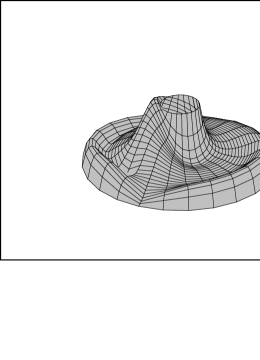
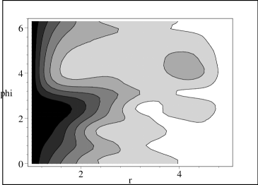
Figure 10: Regime J, $b=5$, $\operatorname{Re}=320$. Left: graph of the absolute velocity $|{\bf{v}}(r,\theta)|$. Right: contour plot of the absolute velocity.

In Figs. 10–14 various features of the flow regime J are illustrated ($b=5$, $\operatorname{Re}=320$). The contour plots of radial velocity $u(r,\theta)$ and azimuthal velocity $v(r,\theta)$ are presented in Fig. 11. The jet-like area of intensive fluid motion is clearly visible in Fig. 11 (left).

Radial profiles of the absolute velocity $|{\bf{v}}(r,\theta)|$ for fixed $r$ are plotted in Fig. 12 (left), azimuthal profiles of the absolute velocity for fixed $\theta$ are presented in Fig. 12 (right). Azimuthal profiles of velocities $u(r,\theta)$ and $v(r,\theta)$, profiles of vorticity $\Delta\psi(r,\theta)$ and profiles of the stream function perturbation $\psi(r,\theta)$ for $r\,=\,const$ are plotted in Figs. 13–14.

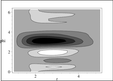
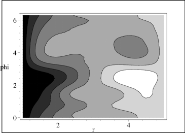
Figure 11: Contour plot of the radial velocity $u(r,\theta)$ and of the azimuthal velocity $v(r,\theta)$. Flow with precessing jet; $b=5$, $\operatorname{Re}=320$.

Profiles of azimuthal velocity for constant $r$ chosen near to the inner or outer circle have the shock-wave type. The jump from larger to smaller values of azimuthal velocity in the direction of precession is observed near the inner circle while the jump from smaller to larger azimuthal velocities is observed near the outer circle. Profiles of radial velocity have the soliton-like shape for all fixed values of $r$. Note that zeros of the radial velocity $u(r,\theta)$ almost coincide with extreme points of the azimuthal velocity $v(r,\theta)$.

Figure 12: Left: radial profiles of the absolute velocity $|{\bf{v}}(r,\theta)|$ at $\theta=(k-1)\pi/3$, where $k$ is the number of the line. Right: azimuthal profiles of $|{\bf{v}}(r,\theta)|$ at $r=1+(3k-1)(b-1)/20$, where $k$ is the number of the line. Flow with precessing jet.

Figure 13: Dependence of radial velocity $u(r,\theta)$ and of azimuthal velocity $v(r,\theta)$ on $\theta$ at $r=1+(3k-1)(b-1)/20$, where $k$ is the number of the line. Flow with precessing jet.

Figure 14: Dependence of vorticity $\Delta\psi(r,\theta)$ and of stream function perturbation $\psi(r,\theta)$ on $\theta$ at $r=1+(3k-1)(b-1)/20$, where $k$ is the number of the line. Flow with precessing jet.

It is interesting to compare results of computation with results of the experiments in which the jet-like flow regimes are observed. In Fig. 15 (published with permission of V. A. Vladimirov and P. V. Denissenko), visualization of the experiment with the jet-like structure is presented ($\operatorname{Re}\sim 56$). The qualitative similarity of the experimental results (Fig. 15, left) and of the numerical results (Fig. 15, right) is obvious. We repeat once again that the quantitative comparison can not be performed because the physical experiment is essentially three-dimensional while the computation considered in this paper is two-dimensional.

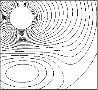
Figure 15: Left: experiment. Free upper surface. Water-glycerol mixture, axial gap thickness $16\cdot 10^{-3}\,m$, radius of the cylinder $10^{-2}\,m$, outer radius of domain $23.2\cdot 10^{-2}\,m$, kinematic viscosity $0.43\cdot 10^{-4}\,m^{2}/s$, rotation speed of the inner cylinder $230\,rpm$, $\operatorname{Re}\sim 56$. Right: Regime J, streamlines, $b=5$, $\operatorname{Re}=320$.

Acknowledgements

This research is partially supported by the Russian Ministry of Education (programme ’Development of the research potential of the high school’, grant 2.1.1/554), by Russian Foundation for Basic Research (grants 07-01-00389, 08-01-00895, and 07-01-92213 NCNIL), and by SRDF grant RUM1-2842-RO-06. This work was done in the framework of European Research Group ’Regular and Chaotic Hydrodynamics’.

References

- [1] V. A. Vladimirov. Proceedings of the First International Conference on Flow Interaction, Hong Kong, 1994. P. 366-369.
- [2] V. A. Vladimirov. Proc. 6th Asian Congress of Fluid Mechanics, Singapore,1995. P. 1584-1587.
- [3] H. K. Moffatt. The asymptotic behavior of solutions of the Navier-Stokes equations near sharp corners. In: Approximate Methods for Navier-Stokes Problems. Lecture Notes in Math., 771, 1980. P. 371-380.
- [4] M. A. Goldshtik. The Eddy Flows. Novosibirsk: Nauka, 1981.
- [5] M. A. Goldshtik, V. N. Shtern, N. I. Yavorskiy. Viscous Flows with Paradoxical Characteristics. Novosibirsk: Nauka, 1989.
- [6] V. Shtern, A. Borissov, F. Hussain. Vortex sinks with axial flow: Solution and applications. J. Phys. Fluids, 9 (10), 1997. P. 2941-2959.
- [7] M. V. Nezlin, E. N. Snezhkin. Rossby vortices and spiral patterns. M.: Nauka, 1990.
- [8] M. Nezlin. Rossby solitary vortices, on giant planets and in the laboratory. Chaos, 4 (2), 1994.
- [9] L. V. Ovsannikov, V. A. Vladimirov, V. Yu. Liapidevsky, N. I. Makarenko, V. N. Nalimov, etc. Nonlinear problems of the theory of surface and internal waves. M.: Nauka, 1985.
- [10] T. B. Benjamin, T. Mullin. Anomalous modes in the Taylor experiment. Proc. R. Soc. Lond. A., 1981. V. 377. P. 221-249.
- [11] K. A. Cliffe. Numerical calculations of two-cell and single-cell Taylor Flows. J. Fluid Mech., 1983. V. 135. P. 219-233.
- [12] M. Lucke, M. Mihelcic, K. Wingerath. Flow in a small annulus between concentric cylinders. J. Fluid Mech., 1984. V. 140. P. 343-353.
- [13] G. Pfister, H. Schmidt, K. A. Cliffe, T. Mullin. Bifurcation phenomena in Taylor-Couette flow in a very short annulus. J. Fluid Mech., 1988. V. 191. P. 1-18.
- [14] J. J. Kobine, T. Mullin. Low-dimensional bifurcation phenomena in Taylor-Couette flow with discrete azimutal symmetry. J. Fluid Mech., 1994. V. 275. P. 379-405.
- [15] V. A. Vladimirov, V. I. Yudovich, M. Yu. Zhukov, P. V. Denissenko. On asymmetric flow structure in a narrow gap between two plates // Proc. of the 13th US National Congress of Applied Mechanics, University of Florida, p. WB1 (1998).
- [16] V. A. Vladimirov, V. I. Yudovich, M. Yu. Zhukov, P. V. Denissenko. On vortex flow in a gap between two parallel plates // Environmental Mathematical Modelling and Numerical Analysis, Rostov-on-Don, 1999. no. 46.
- [17] V. A. Vladimirov, V. I. Yudovich, M. Yu. Zhukov, P. V. Denissenko. On vortex flows in a gap between two parallel plates // 11th Couette-Taylor Workshop ZARM, Univ. of Bremen, 1999.
- [18] V. A. Vladimirov, V. I. Yudovich, M. Yu. Zhukov, P. V. Denissenko. Asymmetric flows induced by a rotating body in a thin layer. Preprint No 3, 14 December, HIMSA, University of Hull. 2001.
- [19] V. M. Ponomarev. On instability of some class of axially symmetric flows of incompressible fluid. Izvestiya AN SSSR. Mekhanika Zhidkosti i Gaza. 1980, No 1. P. 3-9.