On computing the instability index of a non-selfadjoint differential operator associated with coating and rimming flows

Abstract

We study the problem of finding the instability index of certain non-selfadjoint fourth order differential operators that appear as linearizations of coating and rimming flows, where a thin layer of fluid coats a horizontal rotating cylinder. The main result reduces the computation of the instability index to a finite-dimensional space of trigonometric polynomials. The proof uses Lyapunov’s method to associate the differential operator with a quadratic form, whose maximal positive subspace has dimension equal to the instability index. The quadratic form is given by a solution of Lyapunov’s equation, which here takes the form of a fourth order linear PDE in two variables. Elliptic estimates for the solution of this PDE play a key role. We include some numerical examples.

1 Introduction

The stability of steady states is a basic question about the dynamics of any partial differential equation that models the evolution of a physical system. Frequently, the first step is to linearize the system about a given equilibrium. Linearized stability is determined by the spectrum of the resulting differential operator $A$. If $A$ has discrete spectrum, an important quantity is the instability index, $\kappa(A)$, which counts the number of eigenvalues in the right half plane (with multiplicity).

In order to numerically evaluate the instability index of a given differential operator, its computation should be reduced to a problem of linear algebra. Particularly for problems with periodic boundary conditions, it seems natural to restrict $A$ to a finite-dimensional space of trigonometric polynomials. Under what conditions can $\kappa(A)$ be computed from the resulting finite matrix? One difficulty is that the entries of the infinite matrix corresponding to the differential operator $A$ grow with the row and column index, so that any truncation is not a small perturbation.

If $A$ is a self-adjoint semi-bounded differential operator of even order, then the computation of its instability index is well-understood through the classical work of Morse [18] who solved this problem completely in the space of vector functions in one independent variable. The instability index of $A$ agrees with the dimension of the positive cone of the corresponding quadratic form. It is invariant under congruence transformations that replace $A$ with $T^{*}AT$. The instability index can be estimated by variational methods, or computed directly from the zeroes of the corresponding Evans function.

Understanding the spectrum of a non-selfadjoint operator is a much harder problem. It is not at all obvious how to restrict the computation of its instability index to a finite-dimensional subspace, or how to even estimate its dimension. Furthermore, the numerical calculation of eigenvalues can be extremely ill-conditioned even in finite dimensions. One impressive example is the matrix

$$A=\left(\begin{array}[]{ccc}10^{4}+1&10^{6}&10^{4}\\ 10^{6}&2&10^{6}\\ -(10^{4})&-(10^{6})&-(10^{4}-1)\\ \end{array}\right)$$

The Matlab function ${\tt eig}(A)$ gives for the eigenvalues the numerical results $\lambda_{1}=-0.8$, $\lambda_{2/3}=2.4\pm 1.7\,i$, which suggests an instability index of $\kappa(A)=2$. However, the accuracy of the computation is poor. Denoting by $V$ the matrix that contains the (numerically computed) eigenvectors in its columns, and by $E$ the diagonal matrix that contains the (numerically computed) eigenvalues, then

$$norm\,(A-VEV^{-1})=7.6\,.$$

On the other hand, $A$ is similar to an upper triangular matrix

$$A=T\left(\begin{array}[]{ccc}1&10^{6}&10^{4}\\ 0&2&10^{6}\\ 0&0&1\end{array}\right)T^{-1}\,,\quad\mbox{where}\ T=\left(\begin{array}[]{ccc}1&0&0\\ 0&1&0\\ 1&0&1\end{array}\right)\,,$$

and we see that actually $\lambda_{1}=\lambda_{2}=1$, $\lambda_{3}=2$ and $\kappa(A)=3$. In contrast, the eigenvalues of the symmetric matrix

$$B=\left(\begin{array}[]{ccc}10^{4}+1&10^{6}&10^{4}\\ 10^{6}&2&-(10^{6})\\ 10^{4}&-(10^{6})&-(10^{4}-1)\\ \end{array}\right)$$

can be determined with the much better computational accuracy

$$norm\,(B-VEV^{-1})=3.6*10^{-10}\,.$$

Note that $B$ differs from $A$ only in the signs of two off-diagonal entries. The chance of encountering a matrix with moderately-sized entries and a badly conditioned eigenvalue problem increases rapidly with the dimension of the matrix (see [14, 24]). Such examples demonstrate that the stability problem for a non-selfadjoint operator cannot be easily solved by direct computations of the spectrum.

In this paper, we examine the computation of the instability index for differential operators of the form

$$A[h]=-h{{}^{\prime\prime\prime\prime}}-\bigl{(}a(x)h\bigr{)}^{\prime\prime}+\bigl{(}b(x)h\bigr{)}^{\prime}-c(x)h\,,$$ (1.1)

acting on $2\pi$-periodic functions. Such operators appear as linearizations of models for thin liquid films moving on the surface of a horizontal rotating cylinder. The resulting flows are called coating, if the fluid is on the outside of the cylinder, and rimming, if the fluid is on the inside of a hollow cylinder. They appear in many applications, including coating of fluorescent light bulbs when a coating solvent is placed inside a spinning glass tube, different type of moulding processes and paper productions.

One would expect the flow to become unstable, if the fluid film is thick enough so that drops of fluid can form on the bottom of the cylinder (in case of a coating flow) or on its ceiling (in case of a rimming flow). In both cases, surface tension and higher rotation speeds should help to stabilize the fluid, but may also allow for more complicated steady states.

The operators in Eq.(1.1) appear as linearizations of the flows about steady states, when the dependence on the longitudinal variable in the cylinder is neglected. Benilov, O’Brien and Sazonov [5] studied the convection-diffusion equation

$$A[h]=\frac{d}{dx}\Bigl{(}h+\varepsilon\sin x\frac{dh}{dx}\Bigr{)}$$

with periodic boundary conditions on $[0,2\pi]$, which corresponds to a singular limit of a rimming flow where surface tension is neglected. This operator has remarkable properties: For $|\varepsilon|<2$, all its eigenmodes are neutrally stable, but the Cauchy problem

$$\frac{d}{dt}h=A[h],\ \ \ h(0)=h_{0}$$

is ill-posed in any Sobolev and Hölder space of $2\pi$-periodic functions. The underlying cause is the sign change of the diffusion coefficient as $x\to x+\pi$. This phenomenon of explosive instability of a system with purely imaginary spectrum was studied analytically by Chugunova, Karabash and Pyatkov [9], who explained it in terms of the absence of the Riesz basis property of the set of eigenfunctions. The spectral and asymptotic properties of $A$ are of interest in operator theory and were analyzed in [12, 26, 8, 10].

One should expect the explosive instability to disappear in complete models that includes the smoothing effect of surface tension. Such models have been proposed, for example, by [20, 21]. In [6, 7], the authors linearized this model about some approximation of a positive steady state solution to obtain

$$A[h](x)=-\frac{d}{dx}\left\{(1-\alpha_{1}\,\cos x)h+\alpha_{2}\,\sin x\frac{dh}{dx}+\alpha_{3}\,\left(\frac{dh}{dx}+\frac{d^{3}h}{dx^{3}}\right)\right\}$$ (1.2)

with periodic boundary conditions. Here, the parameter $\alpha_{1}$ is related to the gravitational drainage, $\alpha_{2}$ is related to the hydrostatic pressure (in lubrication approximation model this coefficient is very small), and the parameter $\alpha_{3}$ describes surface tension effect. They showed numerically that a sufficiently strong surface tension can stabilize the film provided that the other coefficients are not too small. For smaller values of $\alpha_{1}$ and $\alpha_{2}$, capillary effects destabilize the film. The number of unstable eigenvalues of $A$ grows if $\alpha_{3}$ is decreased.

We will consider operators given by Eq. (1.1) acting on $L^{2}[0,2\pi]$ with periodic boundary conditions. We assume that the coefficients $a(x)$, $b(x)$ and $c(x)$ are bounded smooth periodic functions. We will show that the instability index of $A$ is determined by its projection to a sufficiently large finite-dimensional subspace of $L^{2}$. The dimension of the space depends on a suitable norm of the distributional solution $U$ of the partial differential equation

$${\cal A^{*}}U(x,y)=\delta_{y-x}\,$$ (1.3)

with periodic boundary conditions on $[0,2\pi]\times[0,2\pi]$. Here, the differential operator ${\cal A}$ is defined by applying the single-variable differential operator $A$ to the functions $F(\cdot,y)$ and $F(x,\cdot)$ and adding the results; symbolically

$${\cal A}={\cal A}_{x}+{\cal A}_{y}\,.$$

We note that Eq. (1.3) has a unique solution if the spectra of $A$ and $-A^{*}$ are disjoint [2]. Let $U_{0}(x,y)$ be the solution of Eq. (1.3) with $a(x)=b(x)=0$ and $c(x)=1$. We will see below that $U_{0}$ is piecewise smooth, with a jump in the third derivative across the line $x=y$, and that $U(x,y)-U_{0}(x,y)\in{\cal H}^{4}$.

To describe our results, denote by $P_{N}$ the standard projection onto the space of trigonometric polynomials of order $N$,

$$P_{N}[\phi](x)=\sum_{|p|<N}\hat{\phi}(x)e^{ipx}\,.$$ (1.4)

In Proposition 7.1 we show that

$$\kappa(A)=\kappa\bigl{(}P_{N}U^{-1}P_{N}\bigr{)}\,,$$ (1.5)

provided that

$$N^{2}>2M\bigl{(}1+||U(x,y)-U_{0}(x,y)||_{{\cal H}^{4}}\bigr{)}\,.$$

The constant is given by

$$M=0.52\,\bigl{(}||a||_{H^{1}}+||b||_{H^{1}}+||c-1||_{H^{1}}\bigr{)}\,.$$ (1.6)

The significance of Eq. (1.5) is that it allows to compute the instability index of $A$ from the finite matrix that describes the restriction of $U$ to the finite-dimensional subspace

$$\bigl{(}\mbox{Range}\,(I-P)\bigr{)}^{\perp_{U}}=\mbox{Nullspace}\,(P_{N}U)\,.$$ (1.7)

The weakness of this result is that both the condition on $N$ and the computation of the subspace involve the unknown function $U$, which is defined as the solution of a partial differential equation. The existence of such a solution, and its norm, depend sensitively on the spectrum of $A$, which is exactly the unknown quantity we are concerned with.

It is tempting to consider instead the matrix obtained by truncating the Fourier representation of $A$ at a suitable high order $N$. Our main result, Proposition 7.4, guarantees that

$$\kappa(A)=\kappa\bigl{(}P_{N}AP_{N}\bigr{)}\,.$$ (1.8)

provided that

$$N^{2}>M(1+\sqrt{M+1})\bigl{(}1+||U(x,y)-U_{0}(x,y)||_{{\cal H}^{4}}\bigr{)}\,.$$

Note that only the norm of the unknown function enters into the condition on $N$, and that the identity in Eq. (1.8) does not involve $U$ at all.

The selection of $N$ and the problem of estimating this norm will be discussed at the end.

Let us add a few words about the proofs. Our analysis relies on the indefinite quadratic form defined by the self-adjoint operator $U$. Classical results, which will be discussed in the next section, state that

$$\kappa(A)=\kappa(U)\,,$$

and that the positive and negative cones of $U$ contain the invariant subspaces associated with the spectrum of $A$ in the right and left half planes, respectively. The key to Eq. (1.5) is that the quadratic form is negative on high Fourier modes, because the fourth order term in $A$ dominates the lower order derivatives. As part of the argument, we derive an addition formula for the instability index of a self-adjoint operator in terms of its restriction to suitable subspace. The proof of Eq. (1.8) combines Eq. (1.5) with estimates for the off-diagonal terms in the Fourier representation for $U$.

One of the possible extensions of our results could be an application of a similar method to obtain the estimations on the size of the finite dimensional truncation in the case of a more general forth order differential operator with the third order derivative term which is absent in 1.2.

2 Lyapunov’s equation

The partial differential equation (1.3) is an instance of Lyapunov’s equation

$$A^{*}U+UA=V\,,$$ (2.1)

which was first considered by Lyapunov in the case where $A$ and $U$ are $n\times n$ matrices, and $V$ is symmetric and positive definite. (In Eq. (1.3), $V=I$.) Assuming that a symmetric matrix $U$ solves Eq. (2.1), Lyapunov proved that all eigenvalues of $A$ have negative real part, if and only if $U$ is negative definite. The follwoing generalization is due to Taussky [22].

Theorem 2.1 (Taussky).

Let $A$ be an $n\times n$ complex matric with characteristic roots $\alpha_{i}$, with $\alpha_{i}+\bar{\alpha}_{k}\neq 0$ for all $i,k=1,\dots n$. Then the unique solution $U$ of Lyapunov’s equation with $V=I$ is nonsingular and satisfies $\kappa(U)=\kappa(A)$.

The problem of obtaining information about the sign of eigenvalues of $A$ in situations where both $V$ and $U$ may be indefinite and have non-trivial kernels remains an area of active research.

Lyapunov’s equation has many applications in stability theory and optimal control. In typical applications, $\kappa(A)=0$, so that the system is asymptotically stable, and $U$ is used to estimate the rate of convergence. Eq. (2.1) is a special case of Sylvester’s equation

$$AX-XB=C\,,$$

which has been studied extensively in Linear Algebra, Operator Theory, and Numerical Analysis. It is known to be uniquely solvable, if and only if the matrices $A$ and $B$ have no eigenvalues in common. In particular, Eq. (2.1) has a unique solution if the spectra of $A$ and $-A^{*}$ are disjoint. Since $V$ is self-adjoint, a unique solution $U$ is automatically self-adjoint as well. These results were extended to bounded operators on infinite-dimensional Hilbert spaces by Daleckii and Krein [11] and to unbounded operators by Belonosov [2, 3].

Before stating Belonosov’s result, we recall that a closed densely defined operator $A$ on a Banach space is sectorial, if the spectrum of $A$ is contained in an open sector

$$S=\bigl{\{}z\in\mathbb{C}\ \,\big{|}\,|\arg(\lambda_{0}-z)|<\theta\bigr{\}}$$

with vertex at $\lambda_{0}\in{\mathbb{R}}$ and opening angle $\theta<\pi/2$, and the resolvent $R_{\lambda}(A)=(A-\lambda I)^{-1}$ is uniformly bounded for $\lambda$ outside $S$. Sectorial operators are precisely the generators of analytic semigroups. The sector $S$ is invariant under similarity transformations, and does not change if the norm on the space is replaced by a equivalent norm.

Theorem 2.2 (Belonosov).

Let $A$ be a sectorial operator on a separable Hilbert space $H$. Assume that

$$\sigma(A)\cap\sigma(-A^{*})=\emptyset\,.$$

Then for any bounded operator $V$ on $H$, the Lyapunov equation (2.1) has a unique solution $U$ in the class of bounded operators on $H$. Then $U$ is invertible in the general sense, i.e. its inverse is densely defined but can be unbounded operator

$$\kappa(A)=\kappa(U)=\kappa(U^{-1})\,.$$

Belonosov actually proved more general existence and uniqueness results for the Sylvester’s equation in Banach spaces.

To explain the geometric meaning of Lyapunov’s equation, we introduce on $H$ the indefinite inner product

$$[\phi,\psi]=\langle U\phi,\psi\rangle\,.$$ (2.2)

If $U$ has trivial nullspace and $\kappa(U)<\infty$, then $H$ equipped with $[\cdot,\cdot]$ is called a Pontryagin space, and will be denoted by $\Pi$. The concepts of orthogonality and adjointness are defined on $\Pi$ in the natural way with respect to the indefinite inner product $[x,y]$. A subspace $X\subset\Pi$ is called positive if $[f,f]>0$ for for every non-zero vector $f\in X$, and negative if $[f,f]<0$ for every non-zero $f\in X$. Maximal positive subspaces have dimension $\kappa(U)$, while maximal negative subspaces have codimension $\kappa(U)$.

Let $\phi(t)=e^{tA}\phi_{0}$ be a solution of the evolution equation

$$\frac{d}{dt}\phi(t)=A\phi(t)\,,\quad\phi(0)=\phi_{0}\,.$$

Lyapunov’s equation guarantees that the value of the quadratic form $Q(\phi)=[\phi,\phi]$ strictly increases with $t$,

$$\frac{d}{dt}Q(\phi(t))=\bigl{\langle}(A^{*}U+UA^{*})\phi(t),\phi(t)\bigr{\rangle}=\bigl{\langle}V\phi(t),\phi(t)\bigr{\rangle}>0\,.$$

Denote by $M_{+}(A)$ the invariant subspace associated with the part of the spectrum of $A$ located in the right half plane. If $\phi\in M_{+}(A)$, then

$$Q(\phi)>\lim_{t\to-\infty}Q\bigl{(}e^{tA}\phi\bigr{)}=0\,,$$

which shows that $M_{+}(A)$ is a positive subspace of $\Pi$. A similar argument with $t\to\infty$ shows that the complementary subspace $M_{-}(A)$, which corresponds to the spectrum of $A$ in the left half plane, is a negative subspace of $\Pi$. Since Eq. (2.1) excludes purely imaginary eigenvalues, these subspaces are maximal, and consequently $\kappa(A)=\kappa(U)$.

One can also interpret Lyapunov’s equation as a dissipativity condition on $A$ with respect to the Pontryagin space $\Pi$. In general, a densely defined linear operator $A$ on $\Pi$ called dissipative if ${\bf Re\,}[Af,f]\leq 0$ for all $f\in{\rm Dom}(A)$. It is maximally dissipative if it has no proper dissipative extension in $\Pi$. Assuming Lyapunov’s equation, we compute for $\phi\neq 0$

$${\bf Re\,}[A\phi,\phi]={\bf Re\,}\langle UA\phi,\phi\rangle=\frac{1}{2}\bigl{\langle}(A^{*}U+UA)\phi,\phi\bigr{\rangle}=\frac{1}{2}\langle V\phi,\phi\rangle>0\,,$$

i.e., $-A$ is dissipative. In this framework, the analogue of Belonosov’s theorem was proven by Azizov [1] (but note that Azizov formulates the result in terms of ${\bf Im\,}$ rather than ${\bf Re\,}$):

Theorem 2.3 (Azizov).

Let $A$ be an operator on $\Pi$ such that $-A$ is maximally dissipative. Then there exist a maximal nonnegative subspace $\Pi_{+}$ and a maximal nonpositive subspace $\Pi_{-}$ of $\Pi$ such that

$${\bf Re\,}\sigma(A|_{\Pi_{+}})\geq 0\,,\quad{\bf Re\,}\sigma(A|_{\Pi_{-}})\leq 0\,.$$

Moreover, we can choose $\Pi_{+}$ and $\Pi_{-}$ to be invariant subspaces for $A$, and

$$\Pi_{+}\supset M_{+}(A)\,,\quad\Pi_{-}\supset M_{-}(A)\,.$$

If, additionally, ${\bf Re\,}[Af,f]>0$ for all nonzero $f\in{\rm Dom}(A)$, then $M_{+}(A)$ and $M_{-}(A)$ are themselves maximal positive and negative subspaces for $\Pi$, respectively, and

$$M_{+}(A)\dot{+}M_{-}(A)=\Pi\,.$$

The second part of Azizov’s theorem implies that $\kappa(A)=\kappa(U)$ provided that $V$ in Eq. (2.1) is positive definite. This agrees with the conclusion of Theorem 2.2, but note the difference in the hypotheses: Belonosov’s assumption that $A$ is sectorial provides resolvent estimates that allow to represent $U$ as a contour integral (thereby proving existence), and the analytic semigroup $e^{tA}$ appears in the proof that $\kappa(A)=\kappa(U)$, as sketched above. In contrast, Azizov’s theorem does not require $A$ to be sectorial, but starts instead from a given solution to Eq. (2.1). In the special case where $\kappa(U)=0$, Theorem 2.3 reduces to a theorem of Phillips that characterizes maximal dissipative operators as generators of strongly continuous contraction semigroups. In particular, the spectrum of $A$ lies in the closed left half plane (see  [25], Corollary 1 in Section IX.4).

In the case where $A$ is a sectorial differential operator of even order on an interval $[a,b]$ Belonosov proved that the solution of Lyapunov’s equation with $V=I$ is given by a self-adjoint bounded operator [4]. His results are formulated for “split” boundary conditions that do not couple the values at the two ends of the interval. Belonosov’s results were extended to second-order sectorial differential operators with non-split boundary conditions by Tersenov [23]. The operators we consider here are of fourth order with periodic boundary conditions.

It is an interesting open question how to take advantage of the freedom to choose an arbitrary positive definite self-adjoint bounded operator $V$ for the right hand side of Eq. (2.1). For instance, if $A$ is a sectorial non-selfadjoint differential operator, can $V$ be chosen in such a way that the solution $U$ is the inverse of a differential operator?

3 Spaces and norms

We start with some estimates for the differential operator in Eq. (1.1). We will work in $L^{2}=L^{2}\bigl{(}[0,2\pi]\bigr{)}$, and will use periodic boundary conditions throughout. The inner product and norm are denoted by

$$\langle f,g\rangle=\int_{0}^{2\pi}f(x)\bar{g}(x)\,dx\,,\quad||f||_{L^{2}}=\left(\int_{0}^{2\pi}|f(x)|^{2}\,dx\right)^{1/2}\,.$$

For the Fourier coefficients we use the conventions

$$\hat{f}(p)=\frac{1}{2\pi}\int_{0}^{2\pi}f(x)e^{-ipx}\,dx\,,\quad f(x)=\sum_{p=-\infty}^{\infty}\hat{f}(p)e^{ipx}\,.$$

In the hope of minimizing confusion, we will denote functions on $[0,2\pi]$ by lowercase letters such as ($f$, $\phi$, …), and functions on the square $[0,2\pi]\times[0,2\pi]$ by uppercase letters ($F$, $\Phi$, ….). Abusing notation, we will identify a function $F(x,y)\in{\cal L}^{2}$ with the corresponding integral operator $F$ on $L^{2}$. By Schwarz’ inequality,

$$|\langle F\phi,\psi\rangle|=\Bigl{|}\int_{0}^{2\pi}\int_{0}^{2\pi}F(x,y)\phi(y)\bar{\psi}(x)\,dydx\Bigr{|}\leq||F(x,y)||_{{\cal L}^{2}}||\phi||_{L^{2}}||\psi||_{L^{2}}\,,$$

and consequently

$$||F||_{L^{2}\to L^{2}}\leq||F(x,y)||_{{\cal L}^{2}}\,.$$ (3.1)

Operators on functions of two variables will be denoted by calligraphic letters $({\cal F},{\cal G},\dots)$. Given a single-variable operator $F$, we denote by ${\cal F}_{x}$ or ${\cal F}_{y}$ the operators that acts on the $x$- or $y$-variable of a function $\Phi(x,y)$ while keeping the other one fixed.

On the Sobolev spaces $H^{s}=H^{s}\bigl{(}[0,2\pi]\bigr{)}$ with periodic boundary conditions, we use the norms

$$||f||_{H^{s}}^{2}=2\pi\sum_{p=-\infty}^{\infty}(1+p^{4})^{s/2}\,|\hat{f}(p)|^{2}\,.$$

The corresponding Sobolev spaces of doubly periodic functions on $[0,2\pi]\times[0,2\pi]$ will be denoted by ${\cal H}^{s}$, and their norms are defined by

$$||F||_{{\cal H}^{s}}^{2}=4\pi^{2}\sum_{p,q=-\infty}^{\infty}(2+p^{4}+q^{4})^{s/2}\,|\hat{F}(p,q)|^{2}\,.$$

Note that for $s=0$, this agrees with the definition of the ${\cal L}^{2}$-norm as the square integral. The choice of the Fourier multipliers $(1+p^{4})^{s/2}$ and $(2+p^{4}+q^{4})^{s/2}$ in place of the standard $(1+p^{2})^{s}$ and $(1+p^{2}+q^{2})^{s}$ allows for an easier comparison between functions of one and two variables. Finally, we denote by $D$ the unique positive definite self-adjoint operator on $L^{2}$ such that

$$D^{4}\phi=\phi^{\prime\prime\prime\prime}+\phi\,.$$ (3.2)

This is a first-order pseudodifferential operator that provides an isometry from $H^{s+1}$ onto $H^{s}$ for every value of $s$.

The domain of the operator $A$ in Eq. (1.2) consists of periodic functions in $H^{4}[0,2\pi]$, and its adjoint is given by

$$A^{*}[f]=-f^{{}^{\prime\prime\prime\prime}}-a(x)f^{\prime\prime}-b(x)f^{\prime}-c(x)f\,.$$

In particular, $A$ is self-adjoint, if $b(x)=a^{\prime}(x)$.

Lemma 3.1.

For any $a\in H^{1}$ and every $\phi\in L^{2}$, we have

$$||a\phi||_{L^{2}}\leq 0.52\,||a||_{H^{1}}||\phi||_{L^{2}}\,.$$

In particular,

$$||A^{*}+D^{4}||_{H^{2}\to L^{2}}\leq M\,,$$

where $M$ is the constant from Eq. (1.6).

Proof.

Since

$$\sum_{p=-\infty}^{\infty}(1+p^{4})^{-1/2}\approx 1.68\,,$$

we have, for $a\in H^{1}$,

$$\sup_{||\phi||_{L^{2}}=1}||a\phi||_{L^{2}}\leq||a||_{L^{\infty}}\leq\Bigl{(}\frac{1}{2\pi}\sum_{p=-\infty}^{\infty}(1+p^{4})^{-1/2}\Bigr{)}^{1/2}||a||_{H^{1}}\leq 0.52\,||a||_{H^{1}}\,.$$

For the second claim, we use that for $\phi\in H^{2}$

$$||(A^{*}+D^{4})\phi||_{L^{2}} \leq ||a(x)\phi^{\prime\prime}||_{L^{2}}+||b(x)\phi^{\prime}||_{L^{2}}+||(c(x)-1)\phi||_{L^{2}}$$

$$\leq ||a||_{L^{\infty}}||\phi||_{H^{2}}+||b||_{L^{\infty}}||\phi||_{H^{1}}+||c-1||_{L^{\infty}}||\phi||_{L^{2}}$$

$$\leq M||\phi||_{H^{2}}\,.$$

∎

Lemma 3.2.

$A$ is sectorial.

Proof.

It suffices to show that the Hausdorff set $\bigl{\{}\langle f,Af\rangle\ \mid\ f\in{\rm Dom}(A),||f||=1\bigr{\}}$ is contained in a closed sector

$$S=\{\lambda_{0}\}\cup\{z\in C:|\arg(\lambda_{0}-z)|\leq\theta\}$$

with some vertex $\lambda_{0}$ and opening angle $\theta<\pi$, and that $A-\lambda_{0}I$ is invertible (see p. 280 of [17]).

Choose

$$\lambda_{0} = \frac{1}{2}\bigl{(}1+\max_{x}\{-a^{\prime\prime}(x)+b^{\prime}(x)-c(x)\}+(\max_{x}[a(x)]_{+})^{2}\bigr{)}$$

$$\theta = \tan^{-1}\bigl{(}\max_{x}|a^{\prime}(x)-b(x)|\bigr{)}\,.$$

We estimate, for $f\in H^{2}$

$${\bf Re\,}\langle f,(\lambda_{0}-A)f\rangle = \int_{0}^{2\pi}|f^{\prime\prime}|^{2}-a(x)|f^{\prime}|^{2}+\Bigl{(}\lambda_{0}+\frac{1}{2}a^{\prime\prime}(x)-\frac{1}{2}b^{\prime}(x)+c(x)\Bigr{)}|f|^{2}\,dx$$

$$\geq 2\pi\sum_{p=-\infty}^{\infty}\frac{1+p^{4}}{2}\,|\hat{f}(p)|^{2}$$

$$= \frac{1}{2}||f||_{H^{2}}^{2}\,.$$

This shows that the spectrum of $A$ lies in the half plane ${\bf Re\,}\,z<\lambda_{0}-\frac{1}{2}$. Similarly,

$$|{\bf Im\,}\langle f,(\lambda_{0}-A)f\rangle| \leq \int_{0}^{2\pi}|a^{\prime}(x)-b(x)|\,|{\bf Im\,}f^{\prime}\bar{f}|\,dx$$

$$\leq 2\pi\max_{x}|a^{\prime}(x)-b(x)|\sum_{p=-\infty}^{\infty}|p|\,|\hat{f}(p)|^{2}\,.$$

For $||f||=1$ it follows that

$$\frac{|{\bf Im\,}\,\left\langle f,(\lambda_{0}-A)f\right\rangle|}{{\bf Re\,}\left\langle f,(\lambda_{0}-A)f\right\rangle}\leq\bigl{(}\max_{x}|a^{\prime}(x)-b(x)|\bigr{)}\,\Bigl{(}\sup_{p\in\mathbb{Z}}\frac{2|p|}{1+p^{4}}\Bigr{)}=\max_{x}|a^{\prime}(x)-b(x)|\,,$$

which yields the claim. ∎

The lemma implies that the Cauchy problem for $A$ has a unique solution for every initial value $h_{0}\in L^{2}$. This solution is analytic in $t$ for $t>0$, and for any fixed $t>0$, the function $h(t,\cdot)\in{\rm Dom}(A)$. If the coefficients of $A$ are analytic, then $h$ is analytic in both variables for $t>0$. An application of the Lax-Milgram theorem similar to Lemma 4.1 below shows that $(\lambda_{0}-A)^{-1}$ maps $L^{2}$ into $H^{2}$. It follows that the resolvent is a compact operator of the Hilbert-Schmidt type, and that the spectrum of $A$ is discrete.

4 The integral kernel $U(x,y)$

Let $A$ be the differential operator from Eq. (1.1). Theorem 2.2 implies that Lyapunov’s equation has a unique solution $U$, provided that the spectra of $A$ and $A^{*}$ are disjoint. Our goal is to show that $U$ admits an integral representation

$$U(f)=\int_{0}^{2\pi}U(x,y)f(y)\,dy\,,$$

and to derive bounds on $U(x,y)$. Equation (2.1) requires that $\left\langle(A^{*}U+UA^{*})\phi,\psi\right\rangle=\langle\phi,\psi\rangle$ for all smooth periodic test functions functions $\phi,\psi$. This means that $U(x,y)$ is a distributional solution of the partial differential equation (1.3).

Let us solve Eq. (1.3) in the special case $A_{0}=-D^{4}$, given by

$$A_{0}[f]=-f^{{}^{\prime\prime\prime\prime}}-f\,.$$

By our choice of norms, $-A_{0}$ defines an isometry from $H^{4}$ onto $L^{2}$. Since $A_{0}$ has constant coefficients, the unique solution can be written as $U_{0}(x,y)=u_{0}(x-y)$, where

$$2A_{0}u_{0}=\delta_{0}\,,$$

in other words, $2U_{0}(x,y)$ is the Green’s function of $A_{0}$ on $[0,2\pi]$ with periodic boundary conditions. One can compute $u_{0}(x)$ explicitly as a linear combination

$$u_{0}(x)=C_{1}\cos\frac{x-\pi}{\sqrt{2}}\cosh\frac{x-\pi}{\sqrt{2}}+C_{2}\sin\frac{x-\pi}{\sqrt{2}}\sinh\frac{x-\pi}{\sqrt{2}}\,,$$

where the coefficients are adjusted so that $u_{0}$ is periodic and twice differentiable, and its third derivative jumps by $-1/2$ at $x=0$. From this representation, it is clear that $U_{0}$ is smooth away from the line $x=y$, and that $U_{0}\in{\cal C}^{2,1}\subset{\cal H}^{3}$. Alternately, we easily obtain from the Fourier representation of $A_{0}$ that $\hat{u}_{0}(p)=-\frac{1}{4\pi(1+p^{4})}$, and

$$U_{0}(x,y)=-\frac{1}{4\pi}\sum_{p=-\infty}^{\infty}\frac{1}{1+p^{4}}e^{ip(x-y)}\,.$$ (4.1)

In particular, $U_{0}(x,y)\in H^{s}$ for all $s<\frac{7}{2}$, and $||U_{0}||_{{\cal H}^{3}}\leq 1$.

It remains to analyze the difference

$$K(x,y):=U(x,y)-U_{0}(x,y)\,.$$

By definition, $K$ solves the partial differential equation

$${\cal A}^{*}K(x,y)=-\bigl{(}{\cal A}^{*}-{\cal A}_{0}\bigr{)}U_{0}(x,y)\,.$$ (4.2)

The second order differential operator ${\cal A}^{*}-{\cal A}_{0}$ maps maps $H^{2}$ into $L^{2}$, see Lemma 3.1. A weak solution of this equation is provided by the next lemma.

Lemma 4.1 (Construction of $K$).

The resolvent of ${\cal A}^{*}$ is compact and maps ${\cal L}^{2}$ into ${\cal H}^{2}$.

Proof.

Let $\lambda_{0}$ be the vertex of the sector computed in Lemma 3.2, and assume that $F(x,y)\in{\cal L}^{2}$. We verify that the equation

$$\bigl{(}2\lambda_{0}-{\cal A}^{*}\bigr{)}K(x,y)=F(x,y)$$

satisfies the assumptions of the Lax-Milgram theorem, as stated in [Evans, PDE, p. 297] [13].

Define a bilinear form on on smooth doubly periodic functions $\Phi,\Psi$

$$B(\Phi,\Psi)=\langle(\Phi,(2\lambda_{0}-{\cal A}^{*})\Psi\rangle_{{\cal L}^{2}}\,.$$

Then $B$ is extended continuously to ${\cal H}^{2}$ by

$$B(\Phi,\Psi)=\langle\Phi,\Psi\rangle_{{\cal H}^{2}}+2\lambda_{0}\langle\Phi,\Psi\rangle_{{\cal L}^{2}}-\left\langle\Phi,({\cal A}^{*}-{\cal A}_{0})\Psi\right\rangle_{{\cal L}^{2}}\,.$$

On the other hand, it follows from Eq. (3) that

$$B(\Phi,\Phi)\geq\frac{1}{2}||\Phi||_{{\cal H}^{2}}^{2}\,.$$

Finally, the map

$$\Phi\mapsto-\langle\Phi,F\rangle_{{\cal L}^{2}}$$

defines a continuous linear form on ${\cal H}^{2}$. The Lax-Milgram theorem asserts that there exists a unique function $K(x,y)\in{\cal H}^{2}$ such that

$$B(K,\Psi)=\left\langle F,\Psi\right\rangle_{{\cal L}^{2}}$$

for all $\Psi\in{\cal H}^{2}$. By the resolvent identity, the equation

$$\bigl{(}{\cal A}^{*}-\lambda\bigr{)}K(x,y)=F(x,y)$$

has a unique weak solution in ${\cal H}^{2}$ for every value of $\lambda$ that is not an eigenvalue of ${\cal A}^{*}$ and every $F(x,y)\in{\cal L}^{2}$. ∎

Lemma 4.2.

If $K(x,y)\in{\cal H}^{2}$ solves Eq. (4.2), then $K(x,y)\in{\cal H}^{4}$, and

$$||K(x,y)||_{{\cal H}^{4}}\leq 2M||U_{0}(x,y)+K(x,y)||_{{\cal H}^{2}}\,,$$

where the constant is given by Eq. (1.6).

Proof.

If $K(x,y)$ solves Eq. (4.2), then

$${\cal A}_{0}K=-({\cal A}^{*}-{\cal A}_{0})(U_{0}+K)\,,$$

and we conclude that

$$||K(x,y)||_{{\cal H}^{4}}\leq||{\cal A}^{*}-{\cal A}_{0}||_{{\cal H}^{2}\to{\cal L}^{2}}||U_{0}+K||_{{\cal H}^{2}}\leq 2||A^{*}-A_{0}||_{H^{2}\to L^{2}}||U_{0}+K||_{{\cal H}^{2}}\,.$$

The proof is completed with Lemma 3.1. ∎

5 Estimates for the operator $U$

In this section, we derive bounds for $U=U_{0}+K$ as an operator on $L^{2}$. Since $K(x,y)\in{\cal H}^{4}$, while $U_{0}(x,y)\in H^{s}$ only for $s<7/2$, the Fourier coefficients of $K(x,y)$ decay more quickly than the Fourier coefficients of $U_{0}(x,y)$. This in turn implies that the restriction of $U$ to high Fourier modes is dominated by $U_{0}$. In this section, we provide the relevant estimates.

As a consequence of the regularity result in Lemma 4.2 we see that $U$ defines a bounded linear operator from $L^{2}$ to $H^{4}$, with

$$||U||_{L^{2}\to H^{4}}\leq||U_{0}||_{L^{2}\to H^{4}}+||K||_{L^{2}\to H^{4}}\leq\frac{1}{2}+||K(x,y)||_{{\cal H}^{4}}\,.$$

We have used that $D_{x}^{4}U_{0}=\frac{1}{2}\delta$ and applied Eq. (3.1) to $D^{4}K(x,y)$.

One attractive property of the ${\cal H}^{4}$-norm is that it depends only on the magnitude of the Fourier coefficients, not on the phases. In contrast, the operator norm

$$||F||_{L^{2}\to H^{4}}=\sup_{||\phi||_{L^{2}}=||\psi||_{L^{2}}=1}\langle D^{4}F\phi,\psi\rangle=4\pi^{2}\sum_{p,q=-\infty}^{\infty}(1+p^{4})\hat{F}(p,q)\hat{\phi}(q)\hat{\psi}(p)$$

can change drastically if we replace $\hat{F}(p,q)$ by $|\hat{F}(p,q)|$. This dependence on cancelations can cause difficulties in estimates: Multiplying the Fourier coefficients of $F$ with factors $\alpha(p,q)\in[0,1]$ will not necessarily decrease the operator norm. On the other hand, the $H^{4}$-norm provides only a rather loose bound on the norm of the corresponding integral operator. For instance, the kernles $U_{0}(x,y)$ (and consequently $U(x,y)$ does not lie in ${\cal H}^{4}$, even though $||U_{0}||_{L^{2}\to H^{4}}=\frac{1}{2}$.

We find it useful to introduce another norm on integral kernels that lies between the ${\cal H}^{4}$-norm (as a function of two variables), and the operator norm (as a linear transformation from $L^{2}$ to $H^{4}$). By construction, this norm depends only on the modulus of the Fourier coefficients.

Lemma 5.1 (Auxiliary norm).

Define, for smooth doubly periodic functions $F$

$$|||F|||:=4\pi^{2}\sup_{||\phi||=||\psi||=1}\sum_{p,q=-\infty}^{\infty}(2+p^{4}+q^{4})|\hat{F}(p,q)|\,|\hat{\phi}(p)|\,|\hat{\psi}(q)|\,.$$

Then

$$|||F|||\leq||F(x,y)||_{{\cal H}^{4}}\,,$$

and

$$|||F|||\geq\max\bigl{\{}||F||_{L^{2}\to H^{4}},||F||_{H^{-4}\to L^{2}},2||F||_{H^{-2}\to H^{2}}\bigr{\}}\,.$$

Proof.

From the Fourier representation, we see that

$$|||F||| \leq \sup_{||\Phi(x,y)||_{{\cal L}^{2}}=1}4\pi^{2}\sum_{p,q=i\infty}^{\infty}\sum_{p,q=-\infty}^{\infty}(2+p^{4}+q^{4})|\hat{F}(p,q)|\,|\hat{\Phi}(p,q)|$$

$$\leq \sup_{||\Phi(x,y)||_{{\cal L}^{2}}=1}\langle{\cal A}_{0}F,\Phi\rangle_{{\cal L}^{2}}$$

$$= ||F(x,y)||_{{\cal H}^{4}}\,.$$

On the other hand,

$$||F||_{L^{2}\to H^{4}}=||D^{4}F||_{L^{2}\to L^{2}}=\sup_{||\phi||=||\psi||=1}\sum_{p,q=-\infty}^{\infty}(1+p^{4})\hat{\phi}(p)\hat{\psi}(q)\hat{F}(p,q)\leq|||F|||\,,$$

and similarly

$$||F||_{H^{-2}\to H^{2}}\leq\frac{1}{2}|||F|||\,,\quad||F||_{H^{-4}\to L^{2}}\leq|||F|||\,.$$

∎

We note that if $F$ has positive Fourier coefficients, then $|||F|||$ agrees with the operator norm of ${\cal A}_{0}F$ as a linear transformation from $L^{2}$ into itself. In particular, $|||U_{0}|||=1$.

Lemma 5.2 (Tail estimate).

Assume that $K(x,y)$ solves Eq. (4.2), and let $M$ be given by Eq. (1.6). Then

$$|||K-P_{N}KP_{N}|||\leq MN^{-2}\bigl{(}|||U_{0}+K|||\bigr{)}\,.$$

Proof.

Using Eq. (4.2) together with the definition of the norm, we obtain

$$|||(K-P_{N}KP_{N}||| = 4\pi^{2}\sup_{||\phi||=||\psi||=1}\ \sum_{|p|\geq N\ \mbox{\scriptsize or}\ |q|\geq N}\ |\hat{\phi}(p)|\,|\hat{\psi}(q)|\,|\widehat{({\cal A}^{*}\!-\!{\cal A}_{0})U}(p,q)|$$

$$\leq \sup_{|p|\geq N\ \mbox{\scriptsize or}\ |q|\geq N}\ \frac{(1+p^{4})^{1/2}+(1+q^{4})^{1/2}}{2+p^{4}+q^{4}}\,M|||U|||$$

$$\leq MN^{-2}\bigl{(}|||U_{0}+K|||\bigr{)}\,.$$

∎

Lemma 5.3.

If $U$ solves Eq. (1.3), then $|||U|||\geq 1$.

Proof.

Write $U=U_{0}+K$, and estimate

$$|||U|||\geq|||(I-P_{N})U_{0}(I-P_{N})|||-|||(I-P_{N})K(I-P_{N})|||\,.$$

The first summand is bounded below by $1$ because ${\cal A}_{0}U_{0}=I$, and the second summand is bounded by $MN^{-2}|||U|||$ according to Lemma 5.2. We conclude that $(1-MN^{-2})|||U|||\geq 1$ for each $N$, and the claim follows upon taking $N\to\infty$. ∎

6 Addition rule for the instability index

We return to the Pontryagin space $\Pi$ introduced in Section 2, with the indefinite inner product given by Eq. (2.2). Let $\Pi_{1}$ be a finite-dimensional subspace of $\Pi$, and let

$$\Pi_{2}=\Pi_{1}^{\perp_{U}}=\bigl{\{}f\in\Pi\ \Big{|}[f,g]=0\ \mbox{for all}\ g\in\Pi_{1}\bigr{\}}$$

be its $U$-orthogonal complement. By construction, $\dim\Pi_{1}=\rm codim\,\Pi_{2}$. The natural question is can we compute $\kappa(U)$ from the restrictions $\kappa(U|_{\Pi_{1}})$ and $\kappa(U|_{\Pi_{2}})$? The difficulty is that $\Pi$ need not be a direct sum of $\Pi_{1}$ and $\Pi_{2}$, because the two subspaces may intersect non-trivially in a subspace where the quadratic form vanishes.

A subspace $X\subset\Pi$ is called neutral, if $[\phi,\phi]=0$ for all $\phi\in X$. Two finite-dimensional neutral subspaces $X$ and $Y$ of $H$ are $\Pi$-skewly linked, if

$$\dim X=\dim Y$$

and the inner product $[.,.]$ does not degenerate on the direct sum $X\dot{+}Y$. In particular, no vector of $X$ different from $0$ is orthogonal to the skewly linked subspace $Y$, and vice versa.

Theorem 6.1 (Theorem 3.4 [16]).

Let $\Pi_{1}$ be an arbitrary subspace of $H$, let $\Pi_{2}$ be its $U$-orthogonal complement, and let $X=\Pi_{1}\cap\Pi_{2}$ be their intersection. There exists a neutral subspace $Y\subset\Pi$ that is skewly linked to $X$ and provides a $U$-orthogonal decomposition

$$\Pi=\Pi_{1}^{\prime}\oplus(X\dot{+}Y)\oplus\Pi_{2}^{\prime}\,$$ (6.1)

where

$$\Pi_{1}=\Pi_{1}^{\prime}\oplus X,\qquad\Pi_{2}=\Pi_{2}^{\prime}\oplus X.$$

The theorem was originally formulated for the case of regular Pontryagin spaces, where the quadratic form $U$ is a bounded operator with bounded inverse. Under the assumption that $\Pi_{1}$ is finite-dimensional, the result easily extends to the situation where the inverse of $U$ is unbounded but densely defined. Although the above decomposition is not unique in general, it yields the following addition formula for instability indices:

Proposition 6.2.

Let $\Pi_{1}$ be a finite-dimensional subspace of $\Pi$, and let $\Pi_{2}$ be its $U$-orthogonal complement, Then its instability index is given by

$$\kappa(U)=\kappa(U|_{\Pi_{1}})+\kappa(U|_{\Pi_{2}})+\dim(\Pi_{1}\cap\Pi_{2})\,.$$

Proof.

Theorem 6.1 provides subspaces $\Pi_{1}^{\prime}$ and $\Pi_{2}^{\prime}$ such that

$$\kappa(U)=\kappa(U|_{\Pi_{1}^{\prime}})+\kappa(U|_{\Pi_{2}^{\prime}})+\kappa(U|_{X\dot{+}Y)})\,.$$

By construction, we have $\kappa(U|_{\Pi_{1}^{\prime}})=\kappa(U|_{\Pi_{1}})$ and $\kappa(U|_{\Pi_{2}^{\prime}})=\kappa(U|_{\Pi_{2}})$. It remains to compute $\kappa(U|_{X\dot{+}Y)})$.

Since $X$ and $Y$ are skewly linked and finite-dimensional, there exists for each basis $\phi_{1},\phi_{2},...\phi_{m}$ of $X$ a basis $\psi_{1},\psi_{2},...\psi_{m}$ of $Y$ such that $[\phi_{i},\psi_{j}]=\delta_{ij}$ ($i,j=1,...,m$). By expanding an arbitrary element $h\in X\dot{+}Y$ as

$$h=\sum\limits_{i=1}^{m}\alpha_{i}\phi_{i}+\sum\limits_{j=1}^{m}\beta_{j}\psi_{j}\,,$$

the indefinite inner product can be expressed as

$$[h,h]=2\sum\limits_{i=1}^{m}\alpha_{i}\beta_{i}=\frac{1}{2}\left(\sum\limits_{i=1}^{m}(\alpha_{i}+\beta_{i})^{2}-\sum\limits_{i=1}^{m}(\alpha_{i}-\beta_{i})^{2}\right)\,.$$

This is an explicit representation of the indefinite inner product in terms of positive and negative squares, which shows that $\kappa(U|_{X\dot{+}Y})=\dim(X)$. ∎

7 Restriction to finite dimensions

We first prove the claim in Eq. (1.5).

Proposition 7.1 (Projecting out high Fourier modes).

Let $A$ be given by Eq. (1.1). Assume that the spectra of $A$ and $-A^{*}$ are disjoint, and let $U(x,y)$ be the kernel of the unique solution of Lyapunov’s equation was constructed in Section 4. If

$$N^{2}>M|||U|||\,,$$ (7.1)

where $M$ is the constant from Eq. (1.6), then

$$\kappa(A)=\kappa(P_{N}U^{-1}P_{N})\,.$$

Proof.

By Theorem 2.2, we have $\kappa(A)=\kappa(U)$. Let $[\phi,\psi]=\langle U\phi,\psi\rangle$ be the indefinite inner product associated with $U$. Choose $\Pi_{2}$ to be the range of $I-P_{N}$, and let $\Pi_{1}=\Pi_{2}^{\perp_{U}}$ be its $U$-orthogonal complement. We will show that

$$\kappa(U)=\kappa(U|_{\Pi_{1}})\,.$$ (7.2)

This will establish the conclusion, because

$$\langle P_{N}U^{-1}P_{N}\phi,\phi\rangle=[U^{-1}P_{N}\phi,U^{-1}P_{N}\phi]\,,$$

and $U$ maps $\Pi_{1}$ isomorphically onto the range of $P_{N}$.

Let us apply $[\cdot,\cdot]$ to $D^{2}\phi$, where $\phi\in H^{2}$ and $D$ is given by Eq. (3.2). Writing $U=U_{0}+K$, and using that $D^{2}U_{0}D^{2}=-\frac{1}{2}I$, we see that

$$\bigl{[}D^{2}\phi,D^{2}\phi]=\bigl{\langle}(U_{0}+K)D^{2}\phi,D^{2}\phi\rangle=-\frac{1}{2}||\phi||^{2}+\langle D^{2}KD^{2}\phi,\phi\rangle\,.$$

We replace $\phi$ with $(I-P_{N})\phi$, and use Lemma 5.2 to obtain

$$\bigl{[}D^{2}(I-P_{N})\phi,D^{2}(I-P_{N})\phi] \leq -\frac{1}{2}\bigl{(}1-|||(I-P_{N})K(I-P_{N})|||\bigr{)}||\phi||^{2}$$

$$\leq -\frac{1}{2}(1-\varepsilon_{N})||(I-P_{N})\phi||^{2}\,.$$

where $\varepsilon_{N}=MN^{-2}|||U|||<1$. It follows that

$$U\big{|}_{\Pi_{2}}\leq(1-\varepsilon_{N})\,U_{0}\big{|}_{\Pi_{2}}<0$$ (7.3)

as quadratic forms on $\Pi_{2}$. In particular, $\kappa(U|_{\Pi_{2}})=0$, $\Pi_{1}\cap\Pi_{2}=\emptyset$, and Eq. (7.2) follows with Theorem 6.1. ∎

For our final result, we want to replace $\Pi_{1}$ by the range of the projection $P_{N}$ from Eq. (1.4). The next two lemmas concern the restriction of $U$ to the range of $P_{N}$.

Lemma 7.2 (Lyapunov equation for $P_{N}AP_{N}$).

Let $A$ be given by Eq. (1.1). Assume that the spectrum of $A$ and $-A^{*}$ are disjoint, and let $U(x,y)$ be the kernel of the unique solution of Lyapunov’s equation that we constructed in Section 4. If

$$N^{4}>M^{2}|||U|||\,,$$

then

$$(P_{N}AP_{N})^{*}(P_{N}UP_{N})+(P_{N}UP_{N})(P_{N}AP_{N})\geq c_{N}P_{N}\,,$$ (7.4)

where $c_{N}=1-M^{2}N^{-4}|||U|||$. In particular,

$$\kappa(P_{N}AP_{N})=\kappa(P_{N}UP_{N})\,.$$

Proof.

For $\phi\in L^{2}$, we write $\phi_{1}=P_{N}\phi$, $\phi_{2}=(I-P_{N})\phi$ and decompose

$$A=\left(\begin{array}[]{cc}A_{11}&A_{12}\\ A_{21}&A_{22}\end{array}\right)\,,\quad U=\left(\begin{array}[]{cc}U_{11}&U_{12}\\ U_{21}&U_{22}\end{array}\right)\,.$$

From Eq. (2.1), we see that $U_{11}$ solves Lyapunov’s equation

$$A_{11}^{*}U_{11}+U_{11}A_{11}=V$$

with $V=I_{11}-A^{*}_{12}U_{21}-U_{12}A_{21}$. We claim that the right hand side is positive definite on the range of $P_{N}$.

To prove this claim, first observe that we can replace $A$ by $A-A_{0}$ and $U$ by $K=U-U_{0}$ in the definition of $V$, because $A_{0}$ and $U_{0}$ are diagonal in the Fourier representation. We estimate

$$||A^{*}_{12}U_{21}+U_{12}A_{21}||_{L^{2}\to L^{2}} = ||P_{N}(A^{*}-A_{0})(I-P_{N})KP_{N}+P_{N}K(I-P_{N})(A-A_{0})P_{N}||_{L^{2}\to L^{2}}$$

$$\leq \sup_{|p|\geq N\ \mbox{\scriptsize or}\ |q|\geq N}\frac{(1+p^{4})^{1/2}+(1+q^{4})^{1/2}}{2+p^{4}+q^{4}}\,M|||K-P_{N}KP_{N}|||$$

$$\leq M^{2}N^{-4}|||U|||$$

by Lemma 5.2. It follows that $V\geq c_{N}P_{N}>0$ as quadratic forms on the range of $P_{N}$. Since $P_{N}UP_{N}$ is a finite matrix, the conclusion of the lemma follows with Taussky’s theorem. ∎

Lemma 7.3.

Under the assumptions of the previous lemma, $P_{N}UP_{N}$ is invertible on the range of $P_{N}$, and

$$||\bigl{(}D^{2}P_{N}UP_{N}D^{2}\bigr{)}^{-1}||_{L^{2}\to L^{2}}\leq 2\frac{1+M}{c_{N}}\,.$$

Proof.

Let us write $A_{N}=D^{-2}P_{N}AP_{N}D^{2}$ and $U_{N}=D^{2}P_{N}UP_{N}D^{2}$. By Eq. (7.4), we have

$$A_{N}^{*}U_{N}+U_{N}A_{N}\geq c_{N}D^{4}P_{N}$$

as quadratic forms on the range of $P_{N}$. Here, $c_{N}=1-M^{2}N^{-4}|||U|||$, as in Lemma 7.2. We apply this inequality to an eigenfunction $\phi_{0}$ of $U_{N}$

$$2\lambda_{0}{\bf Re\,}\langle A_{N}^{*}\phi_{0},\phi_{0}\rangle\geq c_{N}\langle D^{2}\phi_{0},D^{2}\phi_{)}\rangle\,,$$

where $\lambda_{0}$ is the corresponding eigenvalue. Writing $\phi_{0}=D^{-2}\psi_{0}$, and using once more Lemma 5.2, we conclude that

$$||U_{N}||_{L^{2}\to L^{2}}\leq 2\sup_{\psi\in L^{2}}\frac{{\bf Re\,}\langle A_{N}^{*}D^{-2}\psi,D^{-2}\psi\rangle}{c_{N}||\psi||_{L^{2}}^{2}}\leq\frac{2}{c_{N}}||A^{*}D^{-4}||_{L^{2}\to L^{2}}\leq 2\frac{1+M}{c_{N}}\,.$$

∎

We are finally ready for our main result.

Proposition 7.4 (Projection onto trigonometric polynomials).

Let $A$ be a differential operator given by Eq. (1.1). Assume that the spectra of $A$ and $-A^{*}$ are disjoint, and let $U(x,y)$ be the unique weak solution of Eq. (1.3) in ${\cal H}^{2}$. If

$$N^{2}>M\bigl{(}1+\sqrt{1+M}\bigr{)}|||U|||\,,$$ (7.5)

where $M$ is given by Eq. (1.6), then

$$\kappa(A)=\kappa(P_{N}AP_{N})\,.$$

Proof.

Since $U$ solves Lyapunov’s equation, Theorem 2.2 implies that $\kappa(A)=\kappa(U)$, and we already know from Lemma 7.2 that $\kappa(P_{N}AP_{N})=\kappa(P_{N}UP_{N})$. We want to apply Proposition 6.2 in the case where $\Pi_{1}$ is the range of $P_{N}$.

Since $|||U|||\geq 1$ by Lemma 5.3, our assumption implies that $\delta_{N}=MN^{-2}<1$. On

$$\Pi_{2}=\mbox{Range}(P_{N})^{\perp_{U}}=\bigl{\{}\phi\in L^{2}\ |\ U_{11}\phi_{1}+U_{12}\phi_{2}=0\bigr{\}}\,,$$

we compute for the indefinite quadratic form

$$[\phi,\phi] = \langle U_{11}\phi_{1},\phi_{1}\rangle+\langle U_{12}\phi_{2},\phi_{1}\rangle+\langle U_{21}\phi_{1},\phi_{2}\rangle+\langle U_{22}\phi_{2},\phi_{2}\rangle$$

$$= -\bigl{\langle}U_{21}U_{11}^{-1}U_{12}\phi_{2},\phi_{2}\rangle+\langle U_{22}\phi_{2},\phi_{2}\rangle\,.$$

By Eq. (7.3) of Proposition 7.1, the last term is negative on the nullspace of $P_{N}$, and satisfies the bound

$$D^{2}U_{22}D^{2}\leq-\frac{1-\delta_{N}|||U|||}{2}(I-P_{N})$$

as quadratic forms. To estimate the other summand, Lemma 5.2 yields

$$||D^{2}U_{21}D^{2}||_{L^{2}\to L^{2}}\leq\frac{1}{2}|||(I-P)UP|||\leq\frac{\delta_{N}}{2}|||U|||\,,$$

and analogously

$$||D^{2}U_{12}D^{2}||_{L^{2}\to L^{2}}\leq\frac{\delta_{N}}{2}|||U|||\,.$$

The middle factor is controlled with Lemma 7.3 by

$$||\bigl{(}D^{2}P_{N}UP_{N}D^{2}\bigr{)}^{-1}||_{L^{2}\to L^{2}}\leq 2\frac{1+M}{1-\delta_{N}^{2}|||U|||}\,.$$

We arrive at

$$D^{2}\bigl{\{}-U_{21}U_{11}^{-1}U_{12}+U_{22}\bigr{\}}D^{2}\leq-\frac{1}{2}\bigl{(}1-\delta_{N}|||U|||-\frac{\delta_{N}^{2}|||U|||^{2}}{1-\delta_{N}^{2}|||U|||}(1+M)\,.$$

as quadratic forms. Since $\delta_{N}^{2}|||U|||^{2}(1+M)<\bigl{(}1-\delta_{N}|||U|||\bigr{)}^{2}$ by assumption, $U$ is negative definite on $\Pi_{2}$. It follows from Proposition 6.2 that $\kappa(U)=\kappa(P_{N}UP_{N})$, completing the proof. ∎

8 Numerical examples

Before we look at examples, a few words about how to verify the hypothesis on $N$ in Eq. (7.1) or Eq. (7.5). The conditions involve the solution of the partial differential equation 1.3. A useful consequence of Lemmas 5.2 and 5.3 is that for $\delta_{N}:=MN^{{}_{2}}<1$,

$$1\leq|||U|||\leq\frac{1}{1-\delta_{N}}\bigl{(}1+|||P_{N}K|||\bigr{)}\,.$$ (8.1)

This follows by using the triangle inequality

$$|||U_{0}+K|||\leq 1+|||P_{N}KP_{N}|||+|||K-P_{N}KP_{N}|||\,$$

and solving for $P_{N}KP_{N}$ in Lemma 5.2.

We propose two ways to estimate the size of $|||P_{N}UP_{N}|||$.

• Solve the partial differential equation (1.3) by a Galerkin approximation, and use this solution to compute, approximately, the value of $|||U|||$. If Eq. (7.1) is satisfied for some value of $N$ much below the dimension of the Galerkin approximation, we can apply Proposition 7.1, and restrict $U$ to the subspace in Eq. (1.7). A basis for this subspace can be computed by using the Gram-Schmidt algorithm, with the inner product replaced by the indefinite inner product associated with $U$. If even Eq. (7.5) can be satisfied, then we can just restrict $U$ to the range of $P_{N}$.

• Start with a value of $N$ such that $\delta_{N}=MN^{-2}<1$. Write the matrix $P_{N}AP_{N}$ in the Fourier representation, find its eigenvalues, and bring it into triangular form. Solve Lyapunov’s equation

  $$P_{N}A^{*}P_{N}\tilde{U}_{N}+\tilde{U}_{N}P_{N}AP_{N}=I\,$$

  for $U_{N}$. In the Fourier representation, $U_{N}$ is a finite matrix. Compute $\lambda_{max}$, the largest eigenvalue of the matrix

  $$\bigl{(}(2+p^{4}+q^{4})|U_{N}(p,q)-1|\bigr{)}_{|p|,|q|<N}\,.$$

  Then $(1+\lambda_{max})/(1-\delta_{N})$ is our best estimate for $|||U|||$. If the condition in Eq. 7.5 holds with the current value of $N$, we are satisfied and accept the value of $\kappa(A_{N})$ as the instability index for $A$. Else, we increase $N$ accordingly, and repeat the above steps.

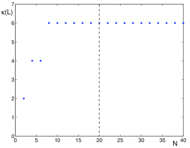
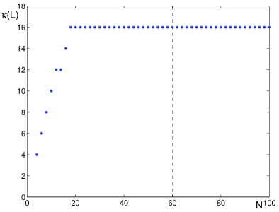
Proposition 7.4 reduces the computation of the stability index of $A$ to a finite-dimensional linear algebra problem. This is illustrated in Fig. 1 for the particular example the operator $A$ from [7], see Eq. (1.2). In this example, we have

$$a(x)=1+\frac{\alpha_{2}}{\alpha_{3}}\sin x\,,\quad b(x)=\frac{1-(\alpha_{1}+\alpha_{2})\cos x}{\alpha_{3}}\,,\quad c(x)=0\,.$$

In place of the constant in Eq. (1.6) we use the slightly smaller value

$$\tilde{M}=\sum_{p=-\infty}^{\infty}\bigl{(}|\hat{a}(p)|+|\hat{b}(p|+|\hat{c}(p)|\bigr{)}=2+\frac{1+\alpha_{1}+2\alpha_{2}}{\alpha_{3}}\,.$$

The results of our computations are shown in Figure 1. We see that if the parameter $\alpha_{3}$ is small, then the surface tension is not strong enough to overcome the gravity and the model is unstable with the number of the unstable eigenvalues growing as the parameter $\alpha_{3}$ decreases.

Figure 1: On the left the parameters: $\alpha_{1}=0.0$, $\alpha_{2}=1$ and $\alpha_{3}=0.02$, resulting in $k\approx 190$; on the right: $\alpha_{1}=0.0$, $\alpha_{2}=1$ and $\alpha_{3}=0.002$, resulting in $k\approx 1875$. The dashed line is showing the suggested cut-off for the dimension of the finite dimensional subspace which is based on the above estimations.

References

- [1] T. Azizov and I.S. Iohvidov, ”Elements of the theory of linear operators in spaces with indefinite metric” (Moscow, Nauka, 1986). Translated as: ”Linear operators in spaces with an indefinite metric”, John Wiley & Sons, 1989.
- [2] V.S. Belonosov, ”On instability indices of unbounded operators. I”, Some Applications of Functional Analysis to Problems in Mathematical Physics [in Russian], Novosibirsk, 2, 25–51, (1984)
- [3] V.S. Belonosov, ”On instability indices of unbounded operators. II”, Some Applications of Functional Analysis to Problems in Mathematical Physics [in Russian], Novosibirsk, 2, 5–33, (1985)
- [4] V.S. Belonosov, ”Instability indices of differential operators. II”, Mat. Sb., 129, No. 4, 494–514, (1986)
- [5] E. S. Benilov, S. B. G. O’Brien, and I. A. Sazonov, ”A new type of instability: explosive disturbances in a liquid film inside a rotating horizontal cylinder”, J. Fluid Mech. 497, 201–224 (2003)
- [6] E. S. Benilov, M. S. Benilov, N. Kopteva, ”Steady rimming flows with surface tension”, J. Fluid Mech. 597, 91–118 (2008)
- [7] E. S. Benilov, N. Kopteva and S. B. G. O’Brien, ”Does surface tension stabilize liquid films inside a rotating horizontal cylinder”, Q. J. Mech. Appl. Math. 58, 158–200 (2005)
- [8] L. Boulton, M. Levitin, and M. Marletta, ”A PT-symmetric periodic problem with boundary and interior singularities”, arXiv:0801.0172v1 [math.SP] (2008)
- [9] M. Chugunova, I.M. Karabash, S.G. Pyatkov, ”On the nature of ill-posedness of the forward-backward heat equation”, preprint, arXiv:0803.2552v2 [math.AP] (2008)
- [10] M. Chugunova, V. Strauss, ”Factorization of the indefinite convection-diffusion operator”, to appear in Math. Reports Acad. Sci. Royal Soc. Canada, (2008)
- [11] Yu. L. Daletskii, M. G. Krein, Stability of solutions to differential equations in Banach space [in Russian], Nauka, Moscow (1970)
- [12] E. B. Davies, ”An indefinite convection-diffusion operator”, LMS J. Comput. Math. 10, 288–306 (2007)
- [13] L. C. Evans, Partial Differential Equations, Graduate Studies in. Mathematics, Vol. 19, American Mathematical Society, Rhode Island (1998)
- [14] S. K. Godunov, Modern Aspect of Linear Algebra, Vol. 175 (AMS Translations, Providence, 1998)
- [15] I. Gohberg and M. G. Krein, Introduction to the theory of linear non-selfadjoint operators, Vol. 18 (AMS Translations, Providence, 1969)
- [16] I.S. Iohvidov, M.G. Krein, and H. Langer, Introduction to the spectral theory of operators in spaces with an indefinite metric (Mathematische Forschung, Berlin, 1982)
- [17] T. Kato, Perturbation theory for linear operators, Springer-Verlag (1976)
- [18] M. Morse, ”Variational Analysis: Critical Extremals and Sturmian Extensions”, John Wiley and ” Sons, Inc., New York; London; Sydney; and Toronto (1973)
- [19] L. S. Pontryagin, ”Symmetric operators in spaces with indefinite metric”, Izv. USSR, Mat. Ser., 8, 243 – 280, (1944)
- [20] V. V. Pukhnachev, ”Motion of a liquid film on the surface of a rotating cylinder in a gravitational field”, Zhuranl Prikladnoi Mekhaniki i Tekhnicheskoi Fiziki, 3, 78 – 88, (1977)
- [21] V. V. Pukhnachev, ”Capillary/gravity film flows on the surface of a rotating cylinder”, Journal of Mathematical Science
- [22] O. Taussky, ”A generalization of a theorem of Lyapunov”, J. Soc. Indust. Appl. Math. 9 1961 640–643.
- [23] Ar. S. Tersenov, ”Solvability of the Lyapunov equation for non-selfadjoint second-order differential operators with nonlocal boundary conditions ”, Siberian Mathematical Journal, 39, No. 5, 1026 – 1042, (1998)
- [24] L.N. Trefethen, Spectral Methods in Matlab (SIAM, Philadelphia, 2000)
- [25] K. Yosida, ”Functional Analysis”, 6th ed., Springer 1980.
- [26] J. Weir, ”An indefinite convection-diffusion operator with real spectrum”, arXiv:0711.1371v1 [math.SP] (2007)