Statistical properties of visibility graph of energy dissipation rates in three-dimensional fully developed turbulence

Abstract

We study the statistical properties of complex networks constructed from time series of energy dissipation rates in three-dimensional fully developed turbulence using the visibility algorithm. The degree distribution is found to have a power-law tail with the tail exponent $\alpha=3.0$. The exponential relation between the number of the boxes $N_{B}$ and the box size $l_{B}$ based on the edge-covering box-counting method illustrates that the network is not self-similar, which is also confirmed by the hub-hub attraction according to the visibility algorithm. In addition, it is found that the skeleton of the visibility network exhibits excellent allometric scaling with the scaling exponent $\eta=1.163\pm 0.005$.

1 Introduction

Turbulence is one of the most challenging fields in physics, and diverse methods have been adopted to investigate the statistical properties of turbulent flows [1, 2]. For instance, the multifractal nature of turbulent flows has been extensively studied based on the structure function analysis of velocity time series [3] and the partition function analysis of energy dissipation rates [4, 5]. Due to the extreme complexity of turbulence, phenomenological investigation of experimental data plays a crucial role in order to gain a better understanding of turbulence, which is fundamental for the construction of models and theories. In this work, we provide a first attempt to study turbulent signals from the complex network perspective, hoping that the ideas, tools, and theories from the flourishing field of complex networks can stimulate the study of turbulence from an alternative point of view. It has been shown that the idea of complex network analysis is able to identify flow patterns and nonlinear dynamics of gas-liquid two-phase flows [6, 7].

Recently, several methods that convert time series into networks have emerged. Zhang et al. introduced a method to deal with the pseudoperiodic time series and found that the structure of the corresponding network depended on the dynamics of the series [8, 9]. In this method, the nodes correspond directly to cycles in the time series, and the edges are determined by the strength of temporal correlation between cycles. This method for pseudoperiodic time series can also be generalized to other time series, where a node is defined by a sub-series of fixed length as an alternative of a cycle, which has been applied to stock prices [10]. Xu et al. proposed another method, which embeds the time series into an appropriate phase space, takes each phase space point as a node in the network, and connects each point with its four nearest neighbors to form a complex network [11]. There are also other mapping methods from time series to networks based on n-tuples of fluctuations [12, 13, 14] or recurrence plots [15, 16].

Lacasa et al. proposed the visibility graph algorithm, which can map all types of time series into networks [17]. In the visibility algorithm, the nodes correspond to the data points of the time series in the same order, and an edge is assigned to connect two nodes if they can “see” each other. It is found that the degree distributions of visibility graphs converted from self-similar time series have power-law tails [17] and the tail exponents depend linearly on the Hurst index of the original time series [18, 19], in which the multifractal nature of the time series has a negligible influence [18]. The visibility algorithm can be simplified to a variant termed the horizontal visibility algorithm, which is solvable [20]. The visibility algorithm has been diversely used to investigate stock market indices [18, 21], human strike intervals [19], the occurrence of hurricanes in the United States [22], and foreign exchange rates [23].

In this paper, we study the statistical properties of complex networks constructed from the energy dissipation rate time series using the visibility algorithm. In Section 2, we describe the turbulence data set. Section 3 briefly describes the visibility graph algorithm. The main results on the degree distribution, the nonfractality and the allometric scaling of the constructed visibility are given in Section 4. We summarize in Section 5.

2 Description of the data set

The velocity data set from three-dimensional fully developed turbulence has been collected at the S1 ONERA wind tunnel by the Grenoble group from LEGI [3]. The mean velocity of the flow is approximately $\langle{v}\rangle=20$m/s (compressive effects are thus negligible). The root-mean-square velocity fluctuations is $v_{\mathtt{rms}}=1.7$m/s, leading to a turbulence intensity equal to $I={v_{\mathtt{rms}}}/{\langle{v}\rangle}=0.0826$. This is sufficiently small to use Taylor’s frozen flow hypothesis. The integral scale is approximately 4m but is difficult to estimate precisely as the turbulent flow is neither isotropic nor homogeneous at these large scales. The Kolmogorov microscale $\eta$ is given by [5]

$$\eta=\left[\frac{\nu^{2}\langle{v}\rangle^{2}}{15\langle(\partial v/\partial t)^{2}\rangle}\right]^{1/4}=0.195~{}{\rm{mm}},$$ (1)

where $\nu=1.5\times 10^{-5}\rm{m^{2}s^{-1}}$ is the kinematic viscosity of air, and $\partial v/\partial t$ is evaluated by its discrete approximation with a time step increment $\partial t=3.5466\times 10^{-5}\rm{s}$ corresponding to the spatial resolution $\delta_{r}=0.72\rm{mm}$ divided by $\langle{v}\rangle$, which is used to transform the data from time to space by applying Taylor’s frozen flow hypothesis. The Taylor scale is given by [5]

$$\lambda=\frac{\langle{v}\rangle v_{\mathtt{rms}}}{\langle(\partial v/\partial t)^{2}\rangle^{1/2}}=16.6~{}{\rm{mm}}.$$ (2)

The Taylor scale is thus about $85$ times the Kolmogorov scale. The Taylor-scale Reynolds number is

$${\rm{Re}}_{\lambda}={\lambda v_{\rm{rms}}}/{\nu}=2000.$$ (3)

This number is actually not constant along the whole data set and fluctuates by about $20\%$. We have checked that the standard scaling laws reported in the literature are recovered with this time series. In particular, we have verified the validity of the power-law scaling $E(k)\sim k^{-\beta}$ with an exponent $\beta$ very close to ${5}/{3}$ over a range more than two orders of magnitude, similar to Fig. 5.4 of [1] provided by Gagne and Marchand on a similar data set from the same experimental group.

Then, we obtained the kinetic energy dissipation rate data using Taylor’s frozen flow hypothesis which replaces a spatial variation of the fluid velocity by a temporal variation measured at a fixed location, and the rate of kinetic energy dissipation at position $i$ is

$$\epsilon_{i}\sim\left[\left(v_{i+1}-v_{i}\right)/\delta_{\ell}\right]^{2}$$ (4)

where $\delta_{\ell}$ is the resolution (translated in spatial scale) of the measurements. Fig. 1 shows a randomly selected segment of 4000 values of the energy dissipation rate time series. The energy dissipation rate time series exhibits multifractal nature [24, 25].

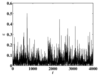
Figure 1: A segment of 4000 data points of the energy dissipation rate time series.

3 Construction of visibility graph

Here, we give a brief introduction of the visibility graph algorithm. For a given time series ($t,\epsilon$), where $t$ is the time variable and $\epsilon$ is the value of energy dissipation rate, a visibility line exists between two points ($t_{a},\epsilon_{a}$) and ($t_{b},\epsilon_{b}$), if any other data ($t_{c},\epsilon_{c}$) placed between them fulfills:

$$\epsilon_{c}<\epsilon_{b}+(\epsilon_{a}-\epsilon_{b})\frac{t_{b}-t_{c}}{t_{b}-t_{a}}~{}.$$ (5)

Fig. 2 illustrates the scheme of the visibility algorithm, where eight points of the energy dissipation rate series are plotted as an example. The height of the vertical lines are the values of energy dissipation rates. The cycles and the dashed lines constitute the visibility graph. The nodes correspond to series data in the same order and an edge connects two nodes if one can be seen from the top of the other. In other words, two nodes are connected if there is visibility between them. Take points 1 and 4 of Fig. 2 as the example to explain the concept of “visibility”. Between 1 and 4, there are two points 2 and 3 which are all under the dashed line from point 1 to point 4, and visibility exists between nodes 1 and 4.

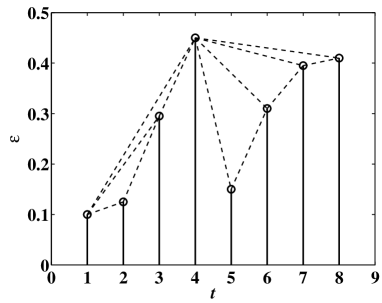
Figure 2: The visibility graph of a short time series.

The networks mapped according to the visibility graph algorithm are connected and undirected. Different time series convert into different networks. It is easy to check that for the time series with monotonously decreasing slopes of all the adjacent points, a chain-like graph will be obtained. According to this algorithm, the dynamics of the time series is conserved in the graph topology. For instance, Lacasa et al. found that periodic time series convert into regular graphs, random time series into random graphs, and fractal series into scale-free graphs [17].

4 Statistical properties of the visibility graph

4.1 Degree distribution

Fig. 3 illustrates the degree distribution $p(k)$ of the visibility graph mapped from the energy dissipation rate series in three-dimensional fully developed turbulence with $10^{6}$ data sets. It is evident that the degree distribution has a power-law tail

$$p(k)\sim k^{-\alpha}~{},$$ (6)

where the exponent is estimated to be $\alpha=3.0$. This power-law distribution is obtained empirically using the method proposed by Clauset, Shalizi and Newman [26]. The power-law exponent is determined by maximum likelihood estimation based on the Kolmogorov-Smirnov statistic [26] and the power-law distribution is statistically significant. It means that the visibility graph under investigation is scale-free. The power-law degree distribution has been found in the visibility graphs mapped from fractal series such as the Brownian motion and Conway series [17]. Fig. 3 shows that multifractal data sets of the energy dissipation rate in turbulence also converts into scale-free networks and the exponent of the degree distribution of the network may depend on the correlation of the series.

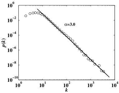
Figure 3: The degree distribution of the visibility graph converted from the time series of the energy dissipation rate series. The line is the best power-law fit of the data.

The power-law degree distribution of the visibility graph has implications for the fractality of the original time series [17, 19, 18]. This is consistent with the well known result that the energy dissipation rate series is statistically self-similar [1]. For nonstationary time series, such as stock price indexes, fractional Brownian motions, Conway series, and strike intervals, there is a linear dependence of the Hurst index on the tail exponent [19, 18]. However, no quantitative relation between the Hurst index of stationary time series and the tail exponent of the degree distribution has been established. Indeed, if we apply rudely the relation in Refs. [19, 18], we will come to the conclusion that the energy dissipation rate series is anticorrelated since the resulting Hurst index is less than $1/2$, which is consistent with the empirical facts [27].

4.2 The visibility graph is not self-similar

The relation between scale-free networks and self-similar networks has been discussed recently [28, 29, 30], and fractal networks seem to exhibit scale-free features while scale-free networks are not always self-similar. The fractal nature of the network can be revealed by the well-known box-counting method. Either the node-covering [28] or the edge-covering [31] box-counting method needs to calculate the minimum number $N_{B}$ of boxes with size $l_{B}$ that can cover all the nodes or edges of the network, where $l_{B}-1$ is the maximum distance of all possible pairs of nodes in each box in the node-covering box-counting method while $l_{B}$ represents the largest distance in the edge-covering method. If the network is self-similar, the minimum number $N_{B}$ of covering boxes scales with respect to box size $l_{B}$ as

$$N_{B}\sim l_{B}^{-D}.$$ (7)

where $D$ is the fractal dimension of the network. In order to obtain the minimum number of the covering box, the simulated annealing algorithm is implemented [31] and the computation may be too enormous for the network mapped from the whole series. In this work, the graph mapped from the 1000 continuous points of the turbulence series are considered to study the fractal feature. Fig. 4 shows the results of the edge-covering box-counting analysis of the visibility graph. As illustrated in Fig. 4, the number of boxes $N_{B}$ decreases exponentially with the size of the boxes $l_{B}$, rather than a power law. Thus, the visibility graph in our work is not fractal.

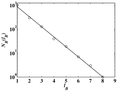
Figure 4: Edge covering box-counting analysis of the visibility graph. $N_{B}$ and $l_{B}$ are in an exponential relation, and the network is non-fractal.

According to Song et al. [28, 29], the network with hubs (the high-degree nodes) attraction will not be self-similar. Whether the interaction is attraction or repulsion among the hubs of the network can be determined from the correlation between the degrees of different nodes. The degree correlation can be quantified by a correlation coefficient $r$ [32, 33]:

$$r=\frac{\langle k_{1}k_{2}\rangle-\langle k_{1}\rangle\langle k_{2}\rangle}{\sigma_{k}^{2}}$$ (8)

where $\sigma_{k}^{2}$ is the variance of all the node degrees, and $k_{1}$, $k_{2}$ are the degrees of the nodes at the ends of all the edges.

It is clear that the degree correlations of adjacent nodes have strong effects on the structure of the network. Networks with positive correlation ($r>0$) tend to have a core-periphery structure, and the hubs are attracted to each other with large probability, while the hubs of a network with negative correlation ($r<0$) are repulsive. In our case, we obtain that $r=0.1204$ for the network mapped from the whole time series. The positive correlation of the whole network indicates that the graph mapped from the energy dissipation rate series is hub-attractive and thus not self-similar. According to the visibility graph method, it is easy to find that large values of the energy dissipation rates correspond to the hubs in the network with large probability, and the points with large values can ”see” each other easily which means that edges exist between the hubs.

More precisely, the correlation coefficient $r$ in Eq. (8) is not a good indicator to determine the fractality of the network. As is explained in Ref. [29], for the property of a higher degree of hub repulsion to be the hallmark of fractality, “the anticorrelation has to appear not only in the original network, but also in the renormalized networks at all length scales.” What is important is not the degree correlation but the scaling of the degree correlation [34]. In addition, some measures of anticorrelation, such as the Pearson coefficient $r$, cannot capture the difference between a fractal and a non-fractal network, since $r$ is not invariant under renormalization [29, 34]. However, positive correlation of degrees using the Pearson coefficient is sufficient to confirm that the network is not fractal.

4.3 Allometric scaling of the visibility graph

The allometric scaling was first proposed in biology [35, 36], and it turns out that the various scalings are characterized by the allometric equation:

$$Y\sim M^{b}$$ (9)

where $Y$ is any physiological, morphological or ecological variable that appears to be correlated with size or body mass $M$, and $b$ is the scaling exponent. Allometric scaling laws have been uncovered in many networks, such as organ metabolic networks [37], food webs [38], world trade/investment webs [39, 40], and so on [41]. The allometric scaling law is proposed in a network based on spanning trees. With one root and plenty of branches and leaves, a tree can be considered as directed from root to leaves. For each node $i$ in the tree, we calculate $A_{i}$ of node $i$ that the summation of value $A$ of its branches along with node $i$ itself

$$A_{i}=\sum_{j}A_{j}+1$$ (10)

and the quantity $C_{i}$ of node $i$ is the sum of the $C$ values of its branches and $A_{i}$

$$C_{i}=\sum_{j}C_{j}+A_{i},$$ (11)

where $j$ is the son node of $i$.

Imagining that there is a flow from the root to the leaves of the tree, the value $A$ stands for the size of node while the value $C$ represents the transport rate through the node. According to Eq. (9), if the property of allometric scaling exists in the tree, the rate $C_{i}$ and the size $A_{i}$ should depend on a power-law relation:

$$C\sim A^{\eta}.$$ (12)

The exponent $\eta$ is a very important parameter of the tree structure. The transportation is more efficient for smaller $\eta$ values. The chain-like trees and star-like trees are the two extremes of the spanning trees, and the value of the allometric exponent $\eta$ is also between that of the two trees. It is easy to obtain that $\eta=2^{-}$ for chain-like trees and $\eta=1^{+}$ for star-like trees. It follows that $1<\eta<2$. We note that not all trees exhibit allometric scaling properties [42, 39], and different spanning trees for the same network may exhibit different allometric features.

For a network, there are various spanning trees with very different structures. In this work, we consider the skeleton [30, 43] of the network. The skeleton is a particular spanning tree which is formed by the edges with largest betweenness centrality of the original network [43]. The skeleton of the scale-free network is also scale-free with a different exponent $\alpha$, and if the original network is self-similar, the skeleton also exhibits self-similarity. To extract the skeleton of a network, we first determine the shortest paths between all pairs of nodes, and the number of times an edge appears in the shortest paths is defined as the weight of the edge,

$$w(E)=\sum_{i,j}c(i,j,E),$$ (13)

where $c(i,j,E)=1$ if the shortest path from node $i$ to $j$ through edge $E$ and $c(i,j,E)=0$ otherwise. The node with the largest degree is considered as the root of the spanning tree. As a first step, we select an edge with the largest weight and add it to the tree if its inclusion will not form any loops. Once all the nodes of the original network are added into the tree, the skeleton is obtained.

We randomly select 100 segments of the time series, each segment having 1000 data points. The 100 sub-series are converted into visibility graphs and their skeleton spanning trees are determined accordingly. Fig. 5 shows the comparison of the scaling behavior between the skeleton and a random spanning tree. The plot of skeleton is shifted upward for clarity and the lines are the best fits of the data. The perfect power-law relations are observed between $C$ and $A$ of all the considered segments, and the line is the best fit of $\ln C$ against $\ln A$. The leaves of the trees ($A=1$, $C=1$) are excluded from the fitting [38]. The exponents of all the skeletons of different segments are around $1.16$ with slight fluctuations, indicating that the allometric scaling property of the visibility graph skeleton remains unchanged at different parts of the turbulence time series. We find that $\eta=1.163\pm 0.005$. We also observe that the data points of the random spanning tree are more dispersive in the scatter plot than those of the skeleton. It is interesting to note that this allometric scaling exponent is quite universal in many different networks [38, 42]. However, the physical implication and the relation to the dynamics of the turbulence signal of this universal topological structure of the visibility graph are unclear.

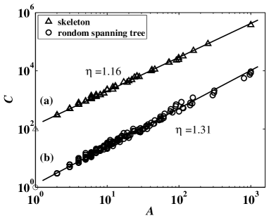
Figure 5: Comparing the allometric scaling behavior of the skeleton and a random spanning tree of the visibility graph mapped from the same series. The lines are the best power-law fits of the data. The data for the skeleton have been shifted upward by two orders of magnitude for clarity.

5 Summary

The visibility graph algorithm is a new method for time series analysis, which converts time series into complex networks. In this way, the time series can be studied from a complex network perspective. The visibility graphs inherit many properties of the associated time series. We have investigated the visibility graphs constructed from the time series of energy dissipation rate in turbulence. We found that the visibility graph has a power-law tail in its degree distribution and is thus scale free, which corresponds to the self-similarity of the energy dissipation rate series. The edge-covering box-counting method shows that the number of boxes decays as an exponential function with respect to the box size, which indicates that the visibility graph is not fractal. The positive degree correlation coefficient $r$ and the visibility algorithm for the turbulence data show hub-hub attraction (rather than hub-hub repulsion) in the network, which explains why there is no self-similarity. In addition, the allometric scaling properties of the visibility graph are studied. We selected skeleton as the particular spanning tree of the network, and the results show that the skeleton exhibits excellent allometric scaling. The networks mapped from various segments of the series of the turbulence have the same scaling exponent $\eta=1.163\pm 0.005$. However, the physical implication of the allometric scaling is not clear. We hope that our analysis will stimulate the study of turbulent signals from the perspective of complex networks.

Acknowledgments:

This work was partially supported by the National Basic Research Program of China (2004CB217703), the Program for Changjiang Scholars and Innovative Research Team in University (IRT0620), and the Program for New Century Excellent Talents in University (NCET-07-0288).

References

- [1] U. Frisch, Turbulence: The Legacy of A.N. Kolmogorov, Cambridge University Press, Cambridge, 1996.
- [2] T. Bohr, M. H. Jensen, G. Paladin, A. Vulpiani, Dynamical Systems Approach to Turbulence, Cambridge University Press, Cambridge, 1998.
- [3] F. Anselmet, Y. Gagne, E. J. Hopfinger, R. A. Antonia, High-order velocity structure functions in turbulent shear flows, J. Fluid Mech. 140 (1984) 63–89.
- [4] B. B. Mandelbrot, Intermittent turbulence in self-similar cascade: Divergence of high moments and dimension of carrier, J. Fluid Mech. 62 (1974) 331–358.
- [5] C. Meneveau, K. R. Sreenivasan, The multifractal nature of turbulent energy dissipation, J. Fluid Mech. 224 (1991) 429–484.
- [6] Z.-K. Gao, N.-D. Jin, Flow-pattern identification and nonlinear dynamics of gas-liquid two-phase flow in complex networks, Phys. Rev. E 79 (2009) 066303. doi:10.1103/PhysRevE.79.066303.
- [7] Z.-K. Gao, N.-D. Jin, Complex network from time series based on phase space reconstruction, Chaos 19 (2009) 033137. doi:10.1063/1.3227736.
- [8] J. Zhang, M. Small, Complex network from pseudoperiodic time series: Topology versus dynamics, Phys. Rev. Lett. 96 (2006) 238701. doi:10.1103/PhysRevLett.96.238701.
- [9] J. Zhang, J.-F. Sun, X.-D. Luo, K. Zhang, T. Nakamura, M. Small, Characterizing pseudoperiodic time series through the complex network approach, Physica D 237 (2008) 2856–2865.
- [10] Y. Yang, H.-J. Yang, Complex network-based time series analysis, Physica A 387 (2008) 1381–1386. doi:10.1016/j.physa.2007.10.055.
- [11] X.-K. Xu, J. Zhang, M. Small, Superfamily phenomena and motifs of networks induced from time series, Proc. Natl. Acad. Sci. U.S.A. 105 (2008) 19601–19605. doi:10.1073/pnas.0806082105.
- [12] P. Li, B.-H. Wang, An approach to Hang Seng Index in Hong Kong stock market based on network topological statistics, Chinese Science Bulletin 51 (2006) 624–629. doi:10.1007/s11434-006-0624-4.
- [13] P. Li, B.-H. Wang, Extracting hidden fluctuation patterns of Hang Seng stock index from network topologies, Physica A 378 (2007) 519–526. doi:10.1016/j.physa.2006.10.089.
- [14] V. Kostakos, Temporal graphs, Physica A 388 (2009) 1007–1023. doi:10.1016/j.physa.2008.11.021.
- [15] N. Marwan, J. F. Donges, Y. Zou, R. V. Donner, J. Kurths, Complex network approach for recurrence analysis of time series, Phys. Lett. A 373 (2009) 4246–4254. doi:10.1016/j.physleta.2009.09.042.
- [16] R. V. Donner, Y. Zou, J. F. Donges, N. Marwan, J. Kurths, Recurrence networks - A novel paradigm for nonlinear time series analysis, New J. Phys. 12 (2010) in press.
- [17] L. Lacasa, B. Luque, F. Ballesteros, J. Luque, J. C. Nuño, From time series to complex networks: The visibility graph, Proc. Natl. Acad. Sci. U.S.A. 105 (2008) 4972–4975. doi:10.1073/pnas.0709247105.
- [18] X.-H. Ni, Z.-Q. Jiang, W.-X. Zhou, Degree distributions of the visibility graphs mapped from fractional Brownian motions and multifractal random walks, Phys. Lett. A 373 (2009) 3822–3826. doi:10.1016/j.physleta.2009.08.041.
- [19] L. Lacasa, B. Luque, J. Luque, J. C. Nuño, The visibility graph: A new method for estimating the Hurst exponent of fractional Brownian motion, EPL 86 (2009) 30001. doi:10.1209/0295-5075/86/30001.
- [20] B. Luque, L. Lacasa, F. Ballesteros, J. Luque, Horizontal visibility graphs: Exact results for random time series, Phys. Rev. E 80 (2009) 046103. doi:10.1103/PhysRevE.80.046103.
- [21] M.-C. Qian, Z.-Q. Jiang, W.-X. Zhou, Universal and nonuniversal allometric scaling behaviors in the visibility graphs of world stock market indices, 0910.2524 (2009).
- [22] J. B. Elsner, T. H. Jagger, E. A. Fogarty, Visibility network of United States hurricanes, Geophys. Res. Lett. 36 (2009) L16702. doi:10.1029/2009GL039129.
- [23] Y. Yang, J.-B. Wang, H.-J. Yang, J.-S. Mang, Visibility graph approach to exchange rate series, Physica A 388 (2009) 4431–4437. doi:10.1016/j.physa.2009.07.016.
- [24] C. Meneveau, K. R. Sreenivasan, Simple multifractal cascade model for fully developed turbulence, Phys. Rev. Lett. 59 (5) (1987) 1424–1427.
- [25] W.-X. Zhou, D. Sornette, Evidence of intermittent cascades from discrete hierarchical dissipation in turbulence, Physica D 165 (2002) 94–125.
- [26] A. Clauset, C. R. Shalizi, M. E. J. Newman, Power-law distributions in empirical data, SIAM Rev. 51 (2009) 661–703. doi:10.1137/070710111.
- [27] C. Liu, W.-X. Zhou, Superfamily classification of nonstationary time series based on DFA scaling exponents, arxiv: 0912.2016 (2009).
- [28] C.-M. Song, S. Havlin, H. A. Makse, Self-similarity of complex networks, Nature 433 (2005) 392–395.
- [29] C.-M. Song, S. Havlin, H. A. Makse, Origins of fractality in the growth of complex networks, Nat. Phys. 2 (2006) 275–281.
- [30] K.-I. Goh, G. Salvi, B. Kahng, D. Kim, Skeleton and fractal scaling in complex networks, Phys. Rev. Lett. 96 (2006) 018701.
- [31] W.-X. Zhou, Z.-Q. Jiang, D. Sornette, Exploring self-similarity of complex cellular networks: The edge-covering method with simulated annealing and log-periodic sampling, Physica A 375 (2007) 741–752.
- [32] M. E. J. Newman, Assortative mixing in networks, Phys. Rev. Lett. 89 (2002) 208701. doi:10.1103/PhysRevLett.89.208701.
- [33] M. Newman, The physics of networks, Phys. Today 61 (11) (2008) 33–38.
- [34] L. K. Gallos, C.-M. Song, H. A. Makse, Scaling of degree correlations and its influence on diffusion in scale-free networks, Phys. Rev. Lett. 100 (2008) 248701. doi:10.1103/PhysRevLett.100.248701.
- [35] G. B. West, J. H. Brown, B. J. Enquist, A general model for the origin of allometric scaling laws in biology, Science 276 (1997) 122–126.
- [36] G. B. West, J. H. Brown, B. J. Enquist, The fourth dimension of life: Fractal geometry and allometric scaling of organisms, Science 284 (1999) 1677–1679.
- [37] M. Santillan, Allometric scaling law in a simple oxygen exchanging network: Possible implications on the biological allometric scaling laws, Eur. Phys. J. B 223 (2003) 249–257.
- [38] D. Garlaschelli, G. Caldarelli, L. Pietronero, Universal scaling relations in food webs, Nature 423 (2003) 165–168.
- [39] W.-Q. Duan, Universal scaling behaviour in weighted trade networks, Eur. Phys. J. B 59 (2007) 271–276. doi:10.1140/epjb/e2007-00279-y.
- [40] D.-M. Song, Z.-Q. Jiang, W.-X. Zhou, Statistical properties of world investment networks, Physica A 388 (2009) 2450–2460. doi:10.1016/j.physa.2009.03.004.
- [41] J. R. Banavar, A. Maritan, A. Rinaldo, Size and form in efficient transportation networks, Nature 399 (1999) 130–132.
- [42] Z.-Q. Jiang, W.-X. Zhou, B. Xu, W.-K. Yuan, Process flow diagram of an ammonia plant as a complex network, AIChE J. 53 (2007) 423–428. doi:10.1002/aic.11071.
- [43] D. H. Kim, J. D. Noh, H. Jeong, Scale-free trees: The skeletons of complex networks, Phys. Rev. E 70 (2004) 046162.