The primordial “$f_{\mathrm{NL}}$” non-Gaussianity, and perturbations beyond the present horizon

Abstract

We show a primordial non-linear (“$f_{\mathrm{NL}}$”) term may produce unphysically large CMB anisotropy for a red-tilted primordial power spectrum ($n<1$), because of coupling to primordial fluctuation on the largest scale. We consider a primordial power spectrum models of a running spectral index, and a transition at very low wavenumbers. We find that only negative running spectral index models are allowed, provided that there is no transition at a low wavenumbers (i.e. $k\ll 1$). For models of a constant spectral index, we find $\log(k_{c}/k_{0})\gtrsim-184$, at $1\sigma$ level, on the transition scale of sharp cut-off models, using recent CMB and SDSS data.

I Introduction

Recently, there have been great successes in measurement of Cosmic Microwave Background (CMB) anisotropy by ground and satellite observations (WMAP5:basic_result, ; WMAP5:powerspectra, ; WMAP5:parameter, ; ACBAR, ; ACBAR2008, ; QUaD1, ; QUaD2, ; QUaD:instrument, ). The five year data of the Wilkinson Microwave Anisotropy Probe (WMAP) WMAP5:basic_result ; WMAP5:powerspectra ; WMAP5:parameter is released and the recent ground-based CMB observations such as the ACBAR ACBAR ; ACBAR2008 and QUaD QUaD1 ; QUaD2 ; QUaD:instrument provide information complementary to the WMAP data. In near future, PLANCK surveyor Planck:sensitivity ; Planck:mission is going to measure CMB temperature and polarization anisotropy with great accuracy over wide range of angular scales. Using the observational data, we are able to impose strong constraints on cosmological models (Modern_Cosmology, ; Inflation, ; Foundations_Cosmology, ), and in particular, on the class of inflation models of very large number of e-folds $N_{e}\gg 100$. They may provide a new window on physics beyond the Planck scale Inflation_Planckian_problem ; Inflation_Planckian_slowroll . Another important feature of the recent CMB observations is testing non-Gaussianity and statistical anisotropy of the CMB sky (cold_spot1, ; cold_spot2, ; cold_spot_wmap3, ; cold_spot_origin, ; Tegmark:Alignment, ; Multipole_Vector, ; Multipole_Vector2, ; Axis_Evil, ; Axis_Evil2, ; Axis_Evil3, ; Power_Asymmetry, ; power_asymmetry_subdegree, ; power_asymmetry_wmap5, ). They provide a unique opportunity to test the modern theories of inflation through the observational data (see for review Non_Gaussianity ).

The fluctuations of the gravitational potential $\Phi(\mathbf{x})$ (equivalent to Bardeen’s gauge invariant variable $\Phi_{H}$ (Bardeen, )) is related to primordial perturbation in complicated ways (Maldacena_fnl, ; WMAP5:Cosmology, ). When considered up to the second order, there exists a nonlinear term $f_{\mathrm{NL}}\,\Phi^{2}_{\mathrm{L}}(\mathbf{x})$, where $f_{\mathrm{NL}}$ is a coupling constant. The nonlinear term $f_{\mathrm{NL}}\,\Phi^{2}_{\mathrm{L}}(\mathbf{x})$ leads to coupling between largest scales and scales relevant to observable Universe. The recent constraint of the WMAP data shows $f_{\mathrm{NL}}\sim 60\pm 30$ (see WMAP3:Gaussianity ; fnl_Yadav ; fnl_Smith ; WMAP5:Cosmology ; fnl_Smith for the recent analysis).

Much of studies have been focused on the behavior of the primordial power spectrum on small scales. In this paper, we focus on the ‘infrared’ asymptotic behavior of a red-tilted ($n<1$) primordial power spectrum. Given the red-tilted primordial power spectra WMAP3:parameter ; WMAP5:Cosmology , coupling to the fluctuation on largest scales may produce unphysically large CMB anisotropy, which could be in disagreement with CMB observational data. There have been attempts to remove the divergence of the nonlinear term by renormalization (fnl_bias, ), and the author notes that the residual k-dependent term, which is not removed by renormalization, is negligible on observable scales for galaxy surveys. Unlike galaxy surveys, the residual k-dependent term produce very large excess power on CMB anisotropy of low multipoles. Not to produce unphysical excess power for CMB anisotropy, we require a primordial power spectrum to satisfy: 1) a spectral index of negative running or 2) a transition at very large scale (e.g. sharp cutoff in the power spectrum at a very low wavenumber). We find at least one of them should be satisfied to make agreement with the recent CMB observational data. As will be discussed in this paper, the imprints of the largest scales due to $f_{\mathrm{NL}}\,\Phi^{2}_{\mathrm{L}}(\mathbf{x})$ term may improve our understanding on the properties of primordial perturbations on the scales larger than the present particle horizon.

The outline of this paper is as follows. In Section II, we discuss the primordial power spectrum associated with a primordial nonlinear (‘$f_{\mathrm{NL}}$’) term. In Section III, we discuss the effect of a ‘$f_{\mathrm{NL}}$’ term on CMB power spectra. In Section IV, we show the primordial power spectrum should satisfy some requirement not to produce unphysically large CMB power spectra. In Section V, we summarize our investigation and discuss prospects.

II the effect of the “$f_{\mathrm{NL}}$” term on a primordial power spectrum

Up to second order, primordial perturbation is given by: (CMB_fnl, ; Komatsu_thesis, ; fnl_simulation, ; WMAP5:Cosmology, ):

$$\Phi(\mathbf{x})=\Phi_{\mathrm{L}}(\mathbf{x})+f_{\mathrm{NL}}\left[\Phi^{2}_{\mathrm{L}}(\mathbf{x})-\langle\Phi^{2}_{\mathrm{L}}(\mathbf{x})\rangle\right],$$ (1)

where $\Phi_{\mathrm{L}}(\mathbf{x})$ is a linear part of primordial perturbation, and $f_{\mathrm{NL}}$ is the non-linear coupling parameter. The last term on the right hand side ensures $\langle\Phi(\mathbf{x})\rangle=0$, and is given by:

$$\langle\Phi^{2}_{\mathrm{L}}(\mathbf{x})\rangle = \int P_{\Phi}(k)\,\frac{d^{3}\mathbf{k}}{(2\pi)^{3}},$$

where

$$P_{\Phi}(k)=\frac{\Delta^{2}_{\mathcal{R}}(k)}{k^{3}}.$$

$\Delta^{2}_{\mathcal{R}}(k)$ is the variance of curvature perturbation per logarithmic interval $d\ln k$ (Inflation, ; WMAP5:Cosmology, ). Using Eq. 1, we find primordial perturbation in Fourier space:

$$\Phi(\mathbf{k})=\Phi_{\mathrm{L}}(\mathbf{k})+\Phi_{\mathrm{NL}}(\mathbf{k}),$$ (2)

where

$$\Phi_{\mathrm{NL}}(\mathbf{k})=$$

$$f_{\mathrm{NL}}\left(\int\Phi_{\mathrm{L}}(\mathbf{k}+\mathbf{p})\Phi^{*}_{\mathrm{L}}(\mathbf{p})\,\frac{d^{3}\mathbf{p}}{(2\pi)^{3}}-(2\pi)^{3}\delta(\mathbf{k})\langle\Phi^{2}_{\mathrm{L}}(\mathbf{x})\rangle\right).$$

In most of inflationary models, $\Phi_{\mathrm{L}}(\mathbf{k})$ follows a Gaussian distribution (Modern_Cosmology, ; Inflation, ; Foundations_Cosmology, ; Komatsu_thesis, ; fnl_simulation, ; WMAP5:Cosmology, ), and hence have the following statistical properties:

$$\langle\Phi_{\mathrm{L}}(\mathbf{k})\rangle = 0,$$ (4)

$$\langle\Phi_{\mathrm{L}}(\mathbf{k})\Phi^{*}_{\mathrm{L}}(\mathbf{k}^{\prime})\rangle = (2\pi)^{3}P_{\Phi}(k)\,\delta(\mathbf{k}-\mathbf{k}^{\prime}),$$ (5)

$$\langle\Phi_{\mathrm{L}}(\mathbf{k}+\mathbf{p})\Phi^{*}_{\mathrm{L}}(\mathbf{p})\rangle = (2\pi)^{3}\delta(\mathbf{k})\,P_{\Phi}(p),$$ (6)

$$\langle\Phi_{\mathrm{L}}(\mathbf{k}+\mathbf{p})\Phi^{*}_{\mathrm{L}}(\mathbf{p})\,\Phi^{*}_{\mathrm{L}}(\mathbf{k}^{\prime}+\mathbf{p}^{\prime})\Phi_{\mathrm{L}}(\mathbf{p}^{\prime})\rangle=(2\pi)^{6}\times$$ (7)

$$\left[P_{\Phi}(k+p)P_{\Phi}(p)\,\delta(\mathbf{k}-\mathbf{k}^{\prime})\left(\delta(\mathbf{p}-\mathbf{p}^{\prime})+\delta(\mathbf{k}+\mathbf{p}+\mathbf{p}^{\prime})\right)\right.$$

$$\left.+\delta(\mathbf{k})\,\delta(\mathbf{k}^{\prime})\,P_{\Phi}(p)\,P_{\Phi}(p^{\prime})\right]$$

Using Eq. II, 4, 5, 6 and 7, we may easily show

$$\langle\Phi_{\mathrm{L}}(\mathbf{k})\Phi^{*}_{\mathrm{NL}}(\mathbf{k}^{\prime})\rangle = 0,$$ (8)

$$\langle\Phi_{\mathrm{NL}}(\mathbf{k})\Phi^{*}_{\mathrm{NL}}(\mathbf{k}^{\prime})\rangle = 8\pi\,(f_{\mathrm{NL}})^{2}\,\delta(\mathbf{k}-\mathbf{k}^{\prime})$$ (9)

$$\times \left[\int P_{\Phi}(k+p)\,P_{\Phi}(p)\,{p}^{2}dp\right].$$

Finally, by using Eq. 2, 5, 8 and 9 we find:

$$\langle\Phi^{*}(\mathbf{k})\Phi(\mathbf{k}^{\prime})\rangle=(2\pi)^{3}\left[P_{\Phi}(k)+P_{\Phi,\mathrm{NL}}(k)\right]\delta(\mathbf{k}-\mathbf{k}^{\prime}),$$

where

$$P_{\Phi,\mathrm{NL}}(k) = \frac{(f_{\mathrm{NL}})^{2}}{\pi^{2}}\int P_{\Phi}(k+k^{\prime})P_{\Phi}(k^{\prime})\>{k^{\prime}}^{2}dk^{\prime}.$$ (10)

III the effect of the ‘$f_{\mathrm{NL}}$’ term on CMB power spectra

The Stokes parameters of CMB anisotropy are conveniently decomposed in terms of spin $0$ and spin $\pm 2$ spherical harmonics:

$$T(\hat{\mathbf{n}}) = \sum_{lm}a_{T,lm}\,Y_{lm}(\hat{\mathbf{n}}),$$

$$Q(\hat{\mathbf{n}})\pm iU(\hat{\mathbf{n}}) = \sum_{l,m}-(a_{E,lm}\pm i\,a_{B,lm})\;{}_{\pm 2}Y_{lm}(\hat{\mathbf{n}}),$$

where $a_{T,lm}$, $a_{E,lm}$ and $a_{B,lm}$ are decomposition coefficients. The decomposition coefficients are related to primordial perturbations as:

$$a_{T,lm} = 4\pi(-\imath)^{l}\int\frac{d^{3}\mathbf{k}}{(2\pi)^{3}}\Phi(\mathbf{k})\,g_{Tl}(k)\,Y^{*}_{lm}(\hat{\mathbf{k}}),$$ (11)

$$a_{E,lm} = 4\pi(-\imath)^{l}\int\frac{d^{3}\mathbf{k}}{(2\pi)^{3}}\Phi(\mathbf{k})\,g_{El}(k)\,Y^{*}_{lm}(\hat{\mathbf{k}}),$$ (12)

$$a_{B,lm} = 4\pi(-\imath)^{l}\int\frac{d^{3}\mathbf{k}}{(2\pi)^{3}}\Phi(\mathbf{k})\,g_{Bl}(k)\,Y^{*}_{lm}(\hat{\mathbf{k}}),$$ (13)

where $g_{Tl}(k)$, $g_{El}(k)$ and $g_{Bl}(k)$ are the radiation transfer functions and can be numerically computed by a computer software CAMB (CAMB, ). In the absence of tensor perturbation, CMB power spectra are given by:

$$C^{TT}_{l} = \frac{2}{\pi}\int k^{2}dk\left[P_{\Phi}(k)+P_{\Phi,\mathrm{NL}}(k)\right]g^{2}_{Tl}(k),$$ (14)

$$C^{EE}_{l} = \frac{2}{\pi}\int k^{2}dk\left[P_{\Phi}(k)+P_{\Phi,\mathrm{NL}}(k)\right]g^{2}_{El}(k),$$ (15)

$$C^{TE}_{l} = \frac{2}{\pi}\int k^{2}dk\left[P_{\Phi}(k)+P_{\Phi,\mathrm{NL}}(k)\right]g_{Tl}(k)g_{El}(k),$$

where $P_{\Phi,\mathrm{NL}}(k)$ is the primordial power spectrum associated with the ‘$f_{\mathrm{NL}}$’ term and given by Eq. 10. Note that CMB anisotropy, excluding the dipole, is sensitive to primordial perturbation of wavenumbers $k\gtrsim 2/\eta_{0}$, where $\eta_{0}$ is the present conformal time.

IV The shape of a Primordial Power Spectrum

Inflation models predict the power spectrum of primordial perturbation nearly follow a power law (CMB_nr, ; Modern_Cosmology, ; Inflation, ; Foundations_Cosmology, ; WMAP1_Inflation, ; WMAP3:parameter, ; WMAP5:Cosmology, ; WMAP5:parameter, ). Since fluctuations, which were once on sub-Planckian scales, are stretched to the observable scales by inflation, we need to consider trans-Planckian effects on a primordial power spectrum (Inflation_Planckian_problem, ; Inflation_Planckian_spectra, ; Inflation_Planckian_note, ; Inflation_Planckian_estimate, ; CMB_Planckian_signature, ; WMAP_oscillation, ; Inflation_Planckian, ; Inflation_initial, ). Since trans-Planckian corrections are highly model-dependent (Planckian_Astrophysics, ; CMB_Planckian_observation, ), we consider general forms of trans-Planckian correction. Following the approach of the WMAP team, we model the variance of curvature perturbation $\Delta^{2}_{\mathcal{R}}(k)$ by two general forms (WMAP3:parameter, ):

$$\Delta^{2}_{\mathcal{R}}(k)=A_{0}\left(\frac{k}{k_{0}}\right)^{n-1}\left[1+\epsilon_{\mathrm{TP}}\cos\left(v\frac{k}{k_{0}}+\phi\right)\right]$$ (17)

$$\Delta^{2}_{\mathcal{R}}(k)=A_{0}\left(\frac{k}{k_{0}}\right)^{n-1}\left[1+\epsilon_{\mathrm{TP}}\cos\left(v\ln{\frac{k}{k_{0}}}+\phi\right)\right]$$ (18)

where the pivot scale $k_{0}$ is set to the WMAP team’s pivot scale $0.002/\mathrm{Mpc}$ (WMAP3:parameter, ), and the spectral index $n$ is given by:

$$n=n(k_{0})+\frac{1}{2}\frac{d\,n}{d\ln k}\,\ln\left(\frac{k}{k_{0}}\right).$$

$\epsilon_{TP}$, $v$, and $\phi$ are the amplitude, the frequency and the phase of trans-Planckian effect. We denote the spectrum in Eq. 17 and 18 respectively as ‘the model I’ and ‘the model II’, which differ in the parametrized form of trans-Planckian corrections. Using Eq. 10, 17 and 18, we find

$$P_{\Phi,\mathrm{NL}}(k)=\frac{(f_{\mathrm{NL}})^{2}}{\pi^{2}}A^{2}_{0}$$ (19)

$$\times \int^{\infty}_{0}\frac{dk^{\prime}}{k_{0}}\left(\frac{k+k^{\prime}}{k_{0}}\right)^{n-4}[1+\epsilon_{\mathrm{TP}}\cos\theta(k+k^{\prime})]$$

$$\times \left(\frac{k^{\prime}}{k_{0}}\right)^{n-2}[1+\epsilon_{\mathrm{TP}}\cos\theta(k^{\prime})]$$

where $\theta(k)=v\frac{k}{k_{0}}+\phi$ for the model I and $\theta=v\ln{\frac{k}{k_{0}}}+\phi$ for the model II.

Most of inflationary models predict that a primordial spectrum is slightly red-tilted (i.e. $n(k_{0})<1$) (Inflation, ; Foundations_Cosmology, ), which is in good agreement with observations (WMAP5:Cosmology, ). Given a slightly red-tiltled spectral index $n<1$, $P_{\Phi,\mathrm{NL}}(k)$ shown in Eq. 19 may become quite large. It increases with decreasing $k$ and has strong $k$-dependenc. This $k$-dependent excess power is not simply removed by renormalization, and may produce very large CMB power spectra on low multipoles (refer to Eq. 14, 15 and LABEL:ClTE). CMB power spectra are well measured by recent satelite and ground observations (ACBAR, ; QUaD_review, ; QUaD1, ; QUaD2, ; QUaD:instrument, ; WMAP5:basic_result, ; WMAP5:powerspectra, ). Not to produce unphysical large excess power, a primordial power spectrum should satisfy some condition, which will be discussed in the following subsections.

IV.1 running spectral index

We consider a running spectral index (i.e. ${d\,n}/{d\ln k}\neq 0$). Since significant contribution to the integral comes from $k^{\prime}/k_{0}\ll 1$, we find $P_{\Phi,\mathrm{NL}}(k)$ for $k\gtrsim 2/\eta_{0}$ and the model I:

$$P_{\Phi,\mathrm{NL}}(k)\approx\frac{(f_{\mathrm{NL}})^{2}}{\pi^{2}}A^{2}_{0}\left(\frac{k}{k_{0}}\right)^{n-4}\left[1+\epsilon_{\mathrm{TP}}\cos\left(v\frac{k}{k_{0}}+\phi\right)\right]$$

$$\times \int^{\infty}_{0}\left(1+\epsilon_{\mathrm{TP}}\cos\phi-\epsilon_{\mathrm{TP}}\,v\,\sin\phi\,\frac{k^{\prime}}{k_{0}}\right)\left(\frac{k^{\prime}}{k_{0}}\right)^{n-2}\frac{dk^{\prime}}{k_{0}}.$$

Note that we have set $k_{\mathrm{max}}$ to $\infty$, because the integrand converges to zero for $k^{\prime}/k_{0}\gg 1$. If ${d\,n}/{d\ln k}<0$, Eq. LABEL:P_NL1 is given by

$$P_{\Phi,\mathrm{NL}}(k) \approx \frac{(f_{\mathrm{NL}})^{2}}{\pi^{2}}A^{2}_{0}\left(\frac{k}{k_{0}}\right)^{n-4}\left[1+\epsilon_{\mathrm{TP}}\cos\left(v\frac{k}{k_{0}}+\phi\right)\right]$$

$$\times \sqrt{\frac{2\pi}{-\alpha}}\left[\left(1+\epsilon_{\mathrm{TP}}\cos\phi\right)\exp\left(-\frac{(n-1)^{2}}{2\alpha}\right)\right.$$

$$\left.-\epsilon_{\mathrm{TP}}\,v\,\sin\phi\exp\left(-\frac{n^{2}}{2\alpha}\right)\right],$$

where $\alpha={d\,n}/{d\ln k}$. On the other hand, if ${d\,n}/{d\ln k}\geq 0$ and the lower integration bound $k_{\mathrm{min}}\to 0$, Eq. LABEL:P_NL1 approach an infinity: $P_{\Phi,\mathrm{NL}}(k)\to\infty$. Hence, we see that ${d\,n}/{d\ln k}<0$ is required to keep CMB power spectra finite.

For $k\gtrsim 2/\eta_{0}$ and the model II, we find:

$$P_{\Phi,\mathrm{NL}}(k)\approx\frac{(f_{\mathrm{NL}})^{2}}{\pi^{2}}A^{2}_{0}\left(\frac{k}{k_{0}}\right)^{n-4}$$

$$\times \left[1+\epsilon_{\mathrm{TP}}\cos\left(v\log\frac{k}{k_{0}}+\phi\right)\right]$$

$$\times \int^{\infty}_{0}\left[1+\epsilon_{\mathrm{TP}}\cos\left(v\log\frac{k}{k_{0}}+\phi\right)\right]\left(\frac{k^{\prime}}{k_{0}}\right)^{n-2}\frac{dk^{\prime}}{k_{0}}$$

$$= \frac{(f_{\mathrm{NL}})^{2}}{\pi^{2}}A^{2}_{0}\left(\frac{k}{k_{0}}\right)^{n-4}\left[1+\epsilon_{\mathrm{TP}}\cos\left(v\log\frac{k}{k_{0}}+\phi\right)\right]$$

$$\times \int^{\infty}_{-\infty}\left[1+\epsilon_{\mathrm{TP}}\cos\left(vx+\phi\right)\right]e^{x(n-1)}dx,$$

where $x=\log(k^{\prime}/k_{0})$. We have also set $k_{\mathrm{max}}$ to $\infty$, because the integrand converges to zero for $k^{\prime}/k_{0}\gg 1$.

If ${d\,n}/{d\ln k}<0$, we get

$$P_{\Phi,\mathrm{NL}}(k) \approx \frac{(f_{\mathrm{NL}})^{2}}{\pi^{2}}A^{2}_{0}\left(\frac{k}{k_{0}}\right)^{n-4}\left[1+\epsilon_{\mathrm{TP}}\cos\left(v\frac{k}{k_{0}}+\phi\right)\right]$$

$$\times \sqrt{\frac{2\pi}{-\alpha}}\exp\left(-\frac{(n-1)^{2}}{2\alpha}\right)$$

$$\times \left[1+\epsilon_{\mathrm{TP}}\cos\left(\phi-\frac{(n-1)v}{\alpha}\right)\exp\left(\frac{v^{2}}{2\alpha}\right)\right],$$

where $\alpha={d\,n}/{d\ln k}$. On the other hand, if ${d\,n}/{d\ln k}\geq 0$ and the lower integration bound $k_{\mathrm{min}}\to 0$, Eq. LABEL:P_NL1 also approach an infinity: $P_{\Phi,\mathrm{NL}}\to\infty$. Therefore, we require ${d\,n}/{d\ln k}<0$ in running spectral index models. Many inflationary models predict a negative ${d\,n}/{d\ln k}$, and hence meet the requirement, while a few inflationary models fail to satisfy the requirement. For instance, the model of a mass term potential $V(\phi)/V_{0}=1\pm 4\pi G\,|c|\,\phi^{2}$ predicts ${d\,n}/{d\ln k}=0$, and the model of the potential $V(\phi)/V_{0}=1-4\pi G|c|\phi^{2}\,\ln\phi/|Q|$, which belongs to the class of a softly broken SUSY models, predicts ${d\,n}/{d\ln k}>0$. Therefore, these models are in disagreement with observations, provided the primordial power spectrum in Eq. 17 and 18 are valid up to the largest spatial scale.

IV.2 sharp cut-off in the primordial power spectrum

We consider a model of a constant spectral index (i.e. ${d\,n}/{d\ln k}=0$), and discuss some requirement to avoid unphysically large $P_{\mathrm{NL}}$. We may consider a transition in the shape of the primordial power spectrum at very low wavenumber, below which Eq. 17 or 18 are no longer valid. For instance, the WMAP team have considered a model of a sharp cutoff, and found that the cut-off at $k_{c}\sim 3\times 10^{-4}/\mathrm{Mpc}$ makes a slightly better fit (WMAP3:parameter, ). For $k>k_{c}$, we may write Eq. 19 as follows:

$$P_{\Phi,\mathrm{NL}}(k)=\frac{(f_{\mathrm{NL}})^{2}A_{0}}{\pi^{2}}\left(\int^{k_{c}}_{0}\frac{dk^{\prime}}{k_{0}}\left(\frac{k+k^{\prime}}{k_{0}}\right)^{n-4}\right.$$ (21)

$$\times [1+\epsilon_{\mathrm{TP}}\cos\theta(k+k^{\prime})]\;P_{\Phi}(k^{\prime})\left(\frac{k^{\prime}}{k_{0}}\right)^{2}$$

$$+ A_{0}\int^{k_{max}}_{k_{c}}\frac{dk^{\prime}}{k_{0}}\left(\frac{k+k^{\prime}}{k_{0}}\right)^{n-4}[1+\epsilon_{\mathrm{TP}}\cos\theta(k+k^{\prime})]$$

$$\times \left.\left(\frac{k^{\prime}}{k_{0}}\right)^{n-2}[1+\epsilon_{\mathrm{TP}}\cos\theta(k^{\prime})]\right)$$

where $\theta(k)=v\frac{k}{k_{0}}+\phi$ for the model I and $\theta=v\ln{\frac{k}{k_{0}}}+\phi$ for the model II.

Just as the WMAP team did, we consider a sharp cut-off at $k_{c}$, and set $P_{\Phi}(k^{\prime})=0$ for $k^{\prime}<k_{c}$. However, $P_{\Phi}(k^{\prime})$ of $k^{\prime}<k_{c}$ may take on some non-zero value, though they are assumed to differ significantly from Eq. 17 and 18. Therefore, our estimate on a transition scale should be interpreted as a lower bound, since a true $P_{\Phi,\mathrm{NL}}(k)$ is more likely to be higher than that of our sharp cut-off model, and a higher $k_{c}$ is needed to make a true $P_{\Phi,\mathrm{NL}}(k)$ equal to that of our sharp cut-off model. In our sharp cut-off model, Eq. 21 is given by

$$P_{\Phi,\mathrm{NL}}(k)=\frac{(f_{\mathrm{NL}})^{2}}{\pi^{2}}A^{2}_{0}\int^{k_{max}}_{k_{c}}\frac{dk^{\prime}}{k_{0}}\left(\frac{k+k^{\prime}}{k_{0}}\right)^{n-4}$$

$$\times [1+\epsilon_{\mathrm{TP}}\cos\theta(k+k^{\prime})]\left(\frac{k^{\prime}}{k_{0}}\right)^{n-2}[1+\epsilon_{\mathrm{TP}}\cos\theta(k^{\prime})].$$

We have found that $P_{\Phi,\mathrm{NL}}(k)$ of $k\gtrsim 2/\eta_{0}$ is barely affected by the value of $k_{\mathrm{max}}$, as long as $\log(k_{\mathrm{max}}/k_{0})\gtrsim 5$. Hence, we have fixed $k_{\mathrm{max}}$ to $\log(k_{\mathrm{max}}/k_{0})=10$, and numerically computed Eq. IV.2 by Romberg integration method (Numerical_Recipe_C, ).

Figure 1: CMB temperature power spectra of $\log(k_{\mathrm{c}}/k_{0})=-120,-100,-60,-5$ (from the highest curve to the lowest), dots denote the WMAP and the ACBAR data.

Figure 2: CMB TE correlation of $\log(k_{\mathrm{c}}/k_{0})=-120,-100,-60,-5$ (from the highest curve to the lowest), dots denote the WMAP data.

Figure 3: E mode power spectrum of $\log(k_{\mathrm{c}}/k_{0})=-120,-100,-60,-5$ (from the highest curve to the lowest), dots denote the WMAP data.

Figure 4: matter power spectrum of $\log(k_{\mathrm{c}}/k_{0})=-120,-100,-60,-5$ (from the highest to the lowest), dots denote SDSS data.

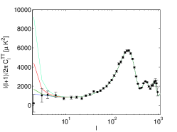
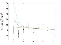
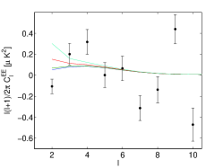
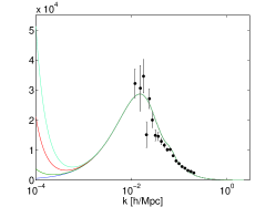
By making a small modification to CAMB, we have computed theoretical CMB and matter power spectrum, in which $P_{\Phi,\mathrm{NL}}(k)$ is taken into account. We show the theoretical CMB power spectra, TE correlation in Fig. 1, 2 and 3. The dots in the same plots denote the WMAP (WMAP5:powerspectra, ) and the ACBAR data (ACBAR2008, ). We may see that anisotropy on largest scales ($l\lesssim 10$) is affected by $P_{\Phi,\mathrm{NL}}$ most. For a E mode power spectrum and TE correlations, we show only low multipoles, since there is no visible effect on higher multipoles. We show a theoretical matter power spectrum and SDSS data in Fig. 4. It also shows that matter inhomogeneities on largest scales ($k\lesssim 10^{-3}h/\mathrm{Mpc}$) are affected by $P_{\mathrm{NL}}$ most. As also noted by (fnl_bias, ), these excess power is, however, negligible on observable scales of the SDSS survey.

Figure 5: Marginalized likelihood (solid lines) and mean likelihood of $\log(k_{c}/k_{0})$ for the model I (top) and II (bottom)

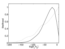
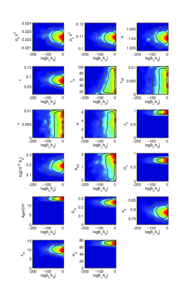
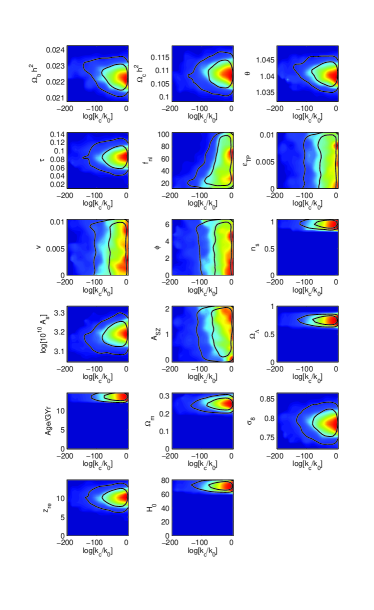
Using a modified CAMB and CosmoMC (CAMB, ; CosmoMC, ), we have estimated $k_{c}$ respectively for the model I and II. For data constraints, we have used the SDSS data SDSS:tech ; SDSS:low_galactic ; SDSS:fifth_data , the recent CMB observations (WMAP + ACBAR + QUaD WMAP5:basic_result ; WMAP5:powerspectra ; ACBAR ; ACBAR2008 ; QUaD1 ; QUaD2 ; QUaD:instrument ), Supernovae data (HST, ; SN_ESSENCE, ; SNLS, ) and Big-Bang Nucleosynthesis (BBN, ). We show the marginalized likelihood (solid lines) and mean likelihood (dotted lines) distribution of $\log(k_{c}/k_{0})$ in Fig. 5. In Fig. 6 and 7, we show the marginalized likelihood distribution in the plane of $\log(k_{c}/k_{0})$ versus other parameters. The $k_{c}$ value of the best-fit cosmological model is $\log(k_{c}/k_{0})=-1.98^{+0.35}_{-168.09}$ and $\log(k_{c}/k_{0})=-1.98^{+0.35}_{-181.81}$ for the model I and II respectively. Note that the confidence interval is marginalized over $\epsilon_{\mathrm{TP}}$, $v$, $\phi$ and $f_{\mathrm{NL}}$ besides the basic $\Lambda$CDM parameters. The best-fit values above do not coincide with the peak of likelihood distribution shown in Fig. 5. We attribute the discrepancy to the deviation of the multi-parameter likelihood function from Gaussian distribution. The central values of our estimated $k_{c}$ are very similar to the cutoff scale found by the WMAP team (WMAP3:parameter, ). Since CMB power spectra are sensitive to $P_{\Phi}(k)$ of $k\gtrsim 2/\eta_{0}$, $k_{c}$ higher than $2/\eta_{0}$ affects CMB power spectra through $P_{\Phi}(k)$ as well as $P_{\Phi,\mathrm{NL}}(k)$. This explains the similarity of the central values to the cutoff scale found by the WMAP team, even though $P_{\Phi,\mathrm{NL}}$ was not taken into account in their analysis. Note that the lower bounds above are associated mainly with $P_{\Phi,\mathrm{NL}}$, since $k_{c}\ll 2/\eta_{0}$.

Figure 6: Marginalized likelihood in the plane of $\log(k_{c}/k_{0})$ versus others parameters for the model I. Two contour lines correspond to 1$\sigma$ and 2$\sigma$ levels.

Figure 7: Marginalized likelihood in the plane of $\log(k_{c}/k_{0})$ versus others parameters for the model II. Two contour lines correspond to 1$\sigma$ and 2$\sigma$ levels.

As shown in Fig. 6 and 7, we find there is little degeneracy between $\log(k_{c}/k_{0})$ and other parameters except for $A_{sz}$. As expected, the best-fit values of the basic $\Lambda$CDM parameters are similar to those of the WMAP concordance model.

IV.3 scale-dependent $f_{\mathrm{NL}}$

The nonlinear coupling parameter ‘$f_{\mathrm{NL}}$’ is a local parameter, and hence possesses some scale-dependence (fnl_review, ). In a single-field inflation, for instance, $f_{\mathrm{NL}}$ in Eq. II is given by (fnl_review, ):

$$f_{\mathrm{NL}}=\frac{5}{6}-3\frac{(\mathbf{k\cdot p})^{2}}{k^{4}}-\frac{2\mathbf{k\cdot p}-p^{2}}{k^{2}}.$$ (23)

In the models of a constant spectral index $n\sim 0.962$ and no transition, all terms of $f_{\mathrm{NL}}$ should have $k$ dependence $k^{\alpha\gtrsim 0.04}$ not to have unphysically large $P_{\mathrm{NL}}$. However, $f_{\mathrm{NL}}$ predicted by most of inflationary models does not have such $k$ dependence. Therefore, we find a scale-dependent $f_{\mathrm{NL}}$ alone does not provide a way to avoid unphysically large $P_{\mathrm{NL}}$.

V discussion

We have shown a primordial non-linear term (‘$f_{\mathrm{NL}}$’ term) may produce unphysically large CMB anisotropy, because of coupling to primordial fluctuation on largest scales. Since such large excess power are not observed in CMB data, we have explored the following minimally extended power law models for a primordial power spectrum to explain the absence of the large excess power.

• A spectral index of a negative running: provided a power law model is valid up to the largest scale (i.e. no transition at a very low wavenumber), running of the spectral index should be negative (i.e. ${d\,n}/{d\ln k}<0$). We may rule out inflationary models of ${d\,n}/{d\ln k}\geq 0$ (e.g. a mass term potential and some models of softly broken SUSY models),

• A transition at a very low wavenumber (e.g. cutoff): provided a spectral index is constant, there should exist some transition at a very low wavenumber, below which the power law is not valid. We have fitted a transition scale of a sharp cut-off model with the recent CMB and SDSS data, and obtained $\log(k_{c}/k_{0})=-1.98^{+0.35}_{-168.09}$ and $\log(k_{c}/k_{0})=-1.98^{+0.35}_{-181.81}$ respectively for two models described by Eq. 17 and 18.

Though it is not clear which condition is true for the primordial power spectrum, it is certain that at least one of two conditions should be met to avoid unphysically large CMB anisotropy.

We shall be able to impose stronger constraints on inflationary models with the data from the upcoming PLANCK surveyor (Planck:sensitivity, ; Planck:mission, ). The improved constraints on a running spectral index of scalar perturbation ${d\,n}/{d\ln k}$, tensor-to-scalar ratio $r$, and the spectral index of tensor perturbation $n_{t}$ will improves our understanding on inflation, and improves our understanding on how unphysically large $P_{\mathrm{NL}}$ is avoided.

VI ACKNOWLEDGMENTS

We are grateful to V. A. Rubakov for helpful discussion. We acknowledge the use of the Legacy Archive for Microwave Background Data Analysis (LAMBDA), ACBAR, QUaD and SDSS data. This work made use of the CosmoMC package. This work was supported by FNU grant 272-06-0417, 272-07-0528 and 21-04-0355.

References

- [1] G. Hinshaw and et al. Five-year wilkinson microwave anisotropy probe (WMAP) observations: Data processing, sky maps, and basic results. 2008. arXiv:0803.0732.
- [2] M. R. Nolta and et al. Five-year Wilkinson Microwave Anisotropy probe (WMAP) observations: Angular power spectra. submitted to Astrophys.J.Suppl., 2008. arXiv:0803.0593.
- [3] J. Dunkley, E. Komatsu, M. R. Nolta, D. N. Spergel, D. Larson, G. Hinshaw, L. Page, C. L. Bennett, B. Gold, N. Jarosik, J. L. Weiland, M. Halpern, R. S. Hill, A. Kogut, M. Limon, S. S. Meyer, G. S. Tucker, E. Wollack, and E. L. Wright. Five-year wilkinson microwave anisotropy probe (wmap) observations: Likelihoods and parameters from the wmap data. ArXiv e-prints, March 2008.
- [4] M. C. Runyan, P. A. R. Ade, R. S. Bhatia, J. J. Bock, M. D. Daub, J. H. Goldstein, C. V. Haynes, W. L. Holzapfel, C. L. Kuo, A. E. Lange, J. Leong, M. Lueker, M. Newcomb, J. B. Peterson, J. Ruhl, G. Sirbi, E. Torbet, C. Tucker, A. D. Turner, and D. Woolsey. Acbar: The arcminute cosmology bolometer array receiver. Astrophys.J.Suppl., 149:265, 2003.
- [5] C. L. Reichardt, P. A. R. Ade, J. J. Bock, J. R. Bond, J. A. Brevik, C. R. Contaldi, M. D. Daub, J. T. Dempsey, J. H. Goldstein, W. L. Holzapfel, C. L. Kuo, A. E. Lange, M. Lueker, M. Newcomb, J. B. Peterson, J. Ruhl, M. C. Runyan, and Z. Staniszewski. High resolution cmb power spectrum from the complete ACBAR data set. To be submitted to Astrophys. J. , 2008. arXiv:0801.1491.
- [6] P. Ade, J. Bock, M. Bowden, M. L. Brown, G. Cahill, J. E. Carlstrom, P. G. Castro, S. Church, T. Culverhouse, R. Friedman, K. Ganga, W. K. Gear, J. Hinderks, J. Kovac, A. E. Lange, E. Leitch, S. J. Melhuish, J. A. Murphy, A. Orlando, R. Schwarz, C. O’Sullivan, L. Piccirillo, C. Pryke, N. Rajguru, B. Rusholme, A. N. Taylor, K. L. Thompson, E. Y. S. Wu, and M. Zemcov. First season quad cmb temperature and polarization power spectra. Astrophys. J. , 674:22, 2008.
- [7] C. Pryke, P. Ade, J. Bock, M. Bowden, M. L. Brown, G. Cahill, P. G. Castro, S. Church, T. Culverhouse, R. Friedman, K. Ganga, W. K. Gear, S. Gupta, J. Hinderks, J. Kovac, A. E. Lange, E. Leitch, S. J. Melhuish, Y. Memari, J. A. Murphy, A. Orlando, R. Schwarz, C. O’Sullivan, L. Piccirillo, N. Rajguru, B. Rusholme, A. N. Taylor, K. L. Thompson, A. H. Turner, E. Y. S. Wu, and M. Zemcov. Second and third season quad cmb temperature and polarization power spectra. submitted to Astrophys. J. , 2008.
- [8] QUaD collaboration: J. Hinderks, P. Ade, J. Bock, M. Bowden, M. L. Brown, G. Cahill, J. E. Carlstrom, P. G. Castro, S. Church, T. Culverhouse, R. Friedman, K. Ganga, W. K. Gear, S. Gupta, J. Harris, V. Haynes, J. Kovac, E. Kirby, A. E. Lange, E. Leitch, O. E. Mallie, S. Melhuish, A. Murphy, A. Orlando, R. Schwarz, C. O’ Sullivan, L. Piccirillo, C. Pryke, N. Rajguru, B. Rusholme, A. N. Taylor, K. L. Thompson, C. Tucker, E. Y. S. Wu, and M. Zemcov. Quad: A high-resolution cosmic microwave background polarimeter. ArXiv e-prints, May 2008.
- [9] J. Clavel and J. A. Tauber. The Planck Mission. In L. I. Gurvits, S. Frey, and S. Rawlings, editors, EAS Publications Series, volume 15 of EAS Publications Series, pages 395–403, 2005.
- [10] J. A. Tauber. The Planck Mission: Overview and Current Status. Astrophysical Letters Communications, 37:145–+, 2000.
- [11] Scott Dodelson. Modern Cosmology. Academic Press, 2nd edition, 2003.
- [12] Andrew R. Liddle and David H. Lyth. Cosmological Inflation and Large-Scale Structure. Cambridge University Press, 1st edition, 2000.
- [13] Viatcheslav Mukhanov. Physical Foundations of Cosmology. Cambridge University Press, 1st edition, 2005.
- [14] J. Martin and R. H. Brandenberger. Trans-Planckian problem of inflationary cosmology. Phys. Rev. D, 63(12):123501–+, June 2001.
- [15] U. H. Danielsson. Transplanckian energy production and slow roll inflation. Phys. Rev. D, 71(2):023516–+, January 2005.
- [16] Angélica de Oliveira-Costa, Max Tegmark, Matias Zaldarriaga, and Andrew Hamilton. The significance of the largest scale CMB fluctuations in WMAP. Phys. Rev. D, 69:063516, 2004.
- [17] C. J. Copi, D. Huterer, and G. D. Starkman. Multipole vectors: A new representation of the CMB sky and evidence for statistical anisotropy or non-Gaussianity at . Phys. Rev. D, 70(4):043515–+, August 2004.
- [18] C. J. Copi, D. Huterer, D. J. Schwarz, and G. D. Starkman. On the large-angle anomalies of the microwave sky. Mon. Not. R. Astron. Soc., 367:79–102, March 2006.
- [19] K. Land and J. Magueijo. Examination of Evidence for a Preferred Axis in the Cosmic Radiation Anisotropy. Physical Review Letters, 95(7):071301–+, August 2005.
- [20] K. Land and J. Magueijo. The Axis of Evil revisited. Mon. Not. R. Astron. Soc., 378:153–158, June 2007.
- [21] A. Rakic and D. J. Schwarz. Correlating anomalies of the microwave sky: The Good, the Evil and the Axis. ArXiv Astrophysics e-prints, March 2007.
- [22] F. K. Hansen, A. J. Banday, K. M. Gorski, H. K. Eriksen, and P. B. Lilje. Power Asymmetry in Cosmic Microwave Background Fluctuations from Full Sky to Sub-degree Scales: Is the Univers Isotropic? submitted to ApJ, December 2008.
- [23] M. Cruz, E. Martínez-González, P. Vielva, and L. Cayón. Detection of a non-Gaussian spot in WMAP. Mon. Not. R. Astron. Soc., 356:29–40, January 2005.
- [24] M. Cruz, M. Tucci, E. Martínez-González, and P. Vielva. The non-Gaussian cold spot in Wilkinson Microwave Anisotropy Probe: significance, morphology and foreground contribution. Mon. Not. R. Astron. Soc., 369:57–67, June 2006.
- [25] M. Cruz, L. Cayón, E. Martínez-González, P. Vielva, and J. Jin. The Non-Gaussian Cold Spot in the 3 Year Wilkinson Microwave Anisotropy Probe Data. Astrophys. J. , 655:11–20, January 2007.
- [26] M. Cruz, E. Martínez-González, P. Vielva, J. M. Diego, M. Hobson, and N. Turok. The CMB cold spot: texture, cluster or void? Mon. Not. R. Astron. Soc., 390:913–919, November 2008.
- [27] F. K. Hansen, A. J. Banday, K. M. Gorski, H. K. Eriksen, and P. B. Lilje. Power Asymmetry in Cosmic Microwave Background Fluctuations from Full Sky to Sub-degree Scales: Is the Universe Isotropic? ArXiv e-prints, December 2008.
- [28] J. Hoftuft, H. K. Eriksen, A. J. Banday, K. M. Gorski, F. K. Hansen, and P. B. Lilje. Increasing evidence for hemispherical power asymmetry in the five-year WMAP data. ArXiv e-prints, March 2009.
- [29] E. Komatsu, N. Afshordi, N. Bartolo, D. Baumann, J. R. Bond, E. I. Buchbinder, C. T. Byrnes, X. Chen, D. J. H. Chung, A. Cooray, P. Creminelli, N. Dalal, O. Dore, R. Easther, A. V. Frolov, K. M. Gorski, J. Khoury, W. H. Kinney, L. Kofman, K. Koyama, L. Leblond, J. . Lehners, J. E. Lidsey, M. Liguori, E. A. Lim, A. Linde, D. H. Lyth, J. Maldacena, S. Matarrese, L. McAllister, P. McDonald, S. Mukohyama, B. Ovrut, H. V. Peiris, A. Riotto, Y. Rodriguez, M. Sasaki, R. Scoccimarro, D. Seery, E. Sefusatti, U. Seljak, L. Senatore, S. Shandera, E. P. S. Shellard, E. Silverstein, A. Slosar, K. M. Smith, A. A. Starobinsky, P. J. Steinhardt, F. Takahashi, M. Tegmark, A. J. Tolley, L. Verde, B. D. Wandelt, D. Wands, S. Weinberg, M. Wyman, A. P. S. Yadav, and M. Zaldarriaga. Non-Gaussianity as a Probe of the Physics of the Primordial Universe and the Astrophysics of the Low Redshift Universe. ArXiv e-prints, February 2009.
- [30] J. M. Bardeen. Gauge-invariant cosmological perturbations. Phys. Rev. D, 22:1882–1905, October 1980.
- [31] J. Maldacena. Non-gaussian features of primordial fluctuations in single field inflationary models. Journal of High Energy Physics, 5:13–+, May 2003.
- [32] E. Komatsu, J. Dunkley, M. R. Nolta, C. L. Bennett, B. Gold, G. Hinshaw, N. Jarosik, D. Larson, M. Limon, L. Page, D. N. Spergel, M. Halpern, R. S. Hill, A. Kogut, S. S. Meyer, G. S. Tucker, J. L. Weiland, E. Wollack, and E. L. Wright. Five-Year Wilkinson Microwave Anisotropy Probe Observations: Cosmological Interpretation. Astrophys.J.Suppl., 180:330–376, February 2009.
- [33] K. M. Smith, L. Senatore, and M. Zaldarriaga. Optimal limits on f_NL^local from WMAP 5-year data. ArXiv e-prints, January 2009.
- [34] A. P. S. Yadav and B. D. Wandelt. Evidence of Primordial Non-Gaussianity () in the Wilkinson Microwave Anisotropy Probe 3-Year Data at 2.8. Physical Review Letters, 100(18):181301–+, May 2008.
- [35] E. Komatsu and et al. Three-year wilkinson microwave anisotropy probe (WMAP) observations: Temperature analysis. Astrophys.J.Suppl., 148:119, 2003.
- [36] D. N. Spergel and et al. Wilkinson Microwave Anisotropy probe WMAP three year results: Implications for cosmology. Astrophys.J.Suppl., 170:377, 2007.
- [37] P. McDonald. Primordial non-Gaussianity: Large-scale structure signature in the perturbative bias model. Phys. Rev. D, 78(12):123519–+, 2008.
- [38] T. Falk, R. Rangarajan, and M. Srednicki. The angular dependence of the three-point correlation function of the cosmic microwave background radiation as predicted by inflationary cosmologies. Astrophys. J. Lett., 403:L1–L3, January 1993.
- [39] E. Komatsu. The Pursuit of Non-Gaussian Fluctuations in the Cosmic Microwave Background. PhD thesis, Tohoku University, 2001.
- [40] M. Liguori, S. Matarrese, and L. Moscardini. High-Resolution Simulations of Non-Gaussian Cosmic Microwave Background Maps in Spherical Coordinates. Astrophys. J. , 597:57–65, November 2003.
- [41] Antony Lewis, Anthony Challinor, and Anthony Lasenby. Efficient computation of CMB anisotropies in closed FRW models. Astrophys. J. , 538:473, 2000. http://camb.info/.
- [42] A. Kosowsky and M. S. Turner. CBR anisotropy and the running of the scalar spectral index. Phys. Rev. D, 52:1739–+, August 1995.
- [43] H. V. Peiris, E. Komatsu, L. Verde, D. N. Spergel, C. L. Bennett, M. Halpern, G. Hinshaw, N. Jarosik, A. Kogut, M. Limon, S. S. Meyer, L. Page, G. S. Tucker, E. Wollack, and E. L. Wright. First-Year Wilkinson Microwave Anisotropy Probe (WMAP) Observations: Implications For Inflation. Astrophys.J.Suppl., 148:213–231, September 2003.
- [44] J. Martin and R. Brandenberger. Dependence of the spectra of fluctuations in inflationary cosmology on trans-Planckian physics. Phys. Rev. D, 68(6):063513–+, September 2003.
- [45] U. H. Danielsson. Note on inflation and trans-Planckian physics. Phys. Rev. D, 66(2):023511–+, July 2002.
- [46] R. Easther, B. R. Greene, W. H. Kinney, and G. Shiu. Generic estimate of trans-Planckian modifications to the primordial power spectrum in inflation. Phys. Rev. D, 66(2):023518–+, July 2002.
- [47] N. Kaloper, M. Kleban, A. Lawrence, and S. Shenker. Signatures of short distance physics in the cosmic microwave background. Phys. Rev. D, 66(12):123510–+, December 2002.
- [48] J. Martin and C. Ringeval. Superimposed oscillations in the WMAP data? Phys. Rev. D, 69(8):083515–+, April 2004.
- [49] C. P. Burgess, J. M. Cline, F. Lemieux, and R. Holman. Are inflationary predictions sensitive to very high energy physics? Journal of High Energy Physics, 2:48–+, February 2003.
- [50] K. Schalm, G. Shiu, and J. P. van der Schaar. Decoupling in an expanding universe: boundary RG-flow affects initial conditions for inflation. Journal of High Energy Physics, 4:76–+, April 2004.
- [51] R. Easther, W. H. Kinney, and H. Peiris. Boundary effective field theory and trans-Planckian perturbations: astrophysical implications. Journal of Cosmology and Astro-Particle Physics, 8:1–+, August 2005.
- [52] R. Easther, W. H. Kinney, and H. Peiris. Observing trans-Planckian signatures in the cosmic microwave background. Journal of Cosmology and Astro-Particle Physics, 5:9–+, May 2005.
- [53] Sarah Church, Peter Ade, James Bock, Melanie Bowden, John Carlstrom, Ken Ganga, Walter Gear, James Hinderks, Wayne Hu, Brian Keating, John Kovac, Andrew Lange, Eric Leitch, Olivier Mallie, Simon Melhuish, Anthony Murphy, Ben Rusholme, Creidhe O’Sullivan, Lucio Piccirillo, Clem Pryke, Andy Taylor, and Keith Thompson. Quest on dasi: a south pole CMB polarization experiment. New Astronomy Reviews, 47:1083, 2003.
- [54] William H. Press, Brian P. Flannery, Saul A. Teukolsky, and William T. Vetterling. Numerical Recipes in C : The Art of Scientific Computing. Cambridge University Press, 2nd edition, 1992.
- [55] Antony Lewis and Sarah Bridle. Cosmological parameters from CMB and other data: a Monte-Carlo approach. Phys. Rev. D, 66:103511, 2002.
- [56] D. G. York and et al. The Sloan Digital Sky Survey: Technical summary. Astron. J., 120:1579, 2000.
- [57] D. Finkbeiner. Sloan Digital Sky Survey imaging of low galactic latitutde fields: Technical summary and data release. Astron. J., 128:2577, 2004.
- [58] J. Adelman-McCarthy and et al. The fifth data release of the sloan digital sky survey. Astrophys.J.Suppl., 172:634–644, October 2007.
- [59] S. Jha, A. G. Riess, and R. P. Kirshner. Improved Distances to Type Ia Supernovae with Multicolor Light-Curve Shapes: MLCS2k2. Astrophys. J. , 659:122–148, 2007.
- [60] G. Miknaitis, G. Pignata, A. Rest, W. M. Wood-Vasey, S. Blondin, P. Challis, R. C. Smith, C. W. Stubbs, N. B. Suntzeff, R. J. Foley, T. Matheson, J. L. Tonry, C. Aguilera, J. W. Blackman, A. C. Becker, A. Clocchiatti, R. Covarrubias, T. M. Davis, A. V. Filippenko, A. Garg, P. M. Garnavich, M. Hicken, S. Jha, K. Krisciunas, R. P. Kirshner, B. Leibundgut, W. Li, A. Miceli, G. Narayan, J. L. Prieto, A. G. Riess, M. E. Salvo, B. P. Schmidt, J. Sollerman, J. Spyromilio, and A. Zenteno. The ESSENCE Supernova Survey: Survey Optimization, Observations, and Supernova Photometry. Astrophys. J. , 666:674–693, 2007.
- [61] P. Astier, J. Guy, N. Regnault, R. Pain, E. Aubourg, D. Balam, S. Basa, R. G. Carlberg, S. Fabbro, D. Fouchez, I. M. Hook, D. A. Howell, H. Lafoux, J. D. Neill, N. Palanque-Delabrouille, K. Perrett, C. J. Pritchet, J. Rich, M. Sullivan, R. Taillet, G. Aldering, P. Antilogus, V. Arsenijevic, C. Balland, S. Baumont, J. Bronder, H. Courtois, R. S. Ellis, M. Filiol, A. C. Gonçalves, A. Goobar, D. Guide, D. Hardin, V. Lusset, C. Lidman, R. McMahon, M. Mouchet, A. Mourao, S. Perlmutter, P. Ripoche, C. Tao, and N. Walton. The Supernova Legacy Survey: measurement of , and w from the first year data set. Astron. Astrophys., 447:31–48, February 2006.
- [62] G. Steigman. Primordial Nucleosynthesis:. Successes and Challenges. International Journal of Modern Physics E, 15:1–35, 2006.
- [63] N. Bartolo, E. Komatsu, S. Matarrese, and A. Riotto. Non-Gaussianity from inflation: theory and observations. Physics Reports, 402:103–266, November 2004.