Recovering Unitarity of Lee Model in Bi-Orthogonal Basis

Abstract

We study how to recover the unitarity of Lee model with the help of bi-orthogonal basis approach, when the physical coupling constant in renormalization exceeds its critical value, so that the Lee’s Hamiltonian is non-Hermitian with respect to the conventional inner product. In a very natural fashion, our systematic approach based on bi-orthogonal basis leads to an elegant definition of inner product with a non-trivial metric, which can overcome all the previous problems in Lee model, such as non-Hermiticity of the Hamiltonian, the negative norm, the negative probability and the non-unitarity of the scattering matrix.

I Introduction

In 1954, T.D. Lee introduced an exactly soluble model to display the necessity of renormalization in quantum field theory (QFT) Lee . It is delicate that with the Lee model, the renormalizations of the mass, wave-function and coupling constant were performed in a closed form Schweber . It is worth remanding that, in the single excitation subspace, the Lee model can be reduced into the Fano model in atom-molecular physics F or the Anderson model of on-site interaction free in condensed matter physics A . With this recognition, the quantum manipulation for the coherent transport in quantum dot array has been investigated based on the Lee model Zhou1 .

Originally, the Lee model describes the reaction processes $V\rightleftarrows N+\theta$, namely, a fermion $V$ transforms to another fermion $N$ by emitting bosonic $\theta$-particle, and vice versa. In the single particle subspace—the $V/N\theta$ sector, the Lee model is exactly solvable. According to the analytic solution, we only need to consider the mass renormalization of the $V$-particle and coupling constant renormalization since the bare single-particle states of $\theta$ and $N$ are both the eigenstates of the Hamiltonian, thus the mass renormalizations of $\theta$ and $N$-particles are not need, and their physical masses equal to the bare masses. In the $V/N\theta$ sector, the eigenstates of the Hamiltonian contain the physical $V$-state and $N\theta$-scattering states.

In the Lee model, the renormalization about $V$-particle results in some perplexing and interesting natures, e.g., the emergence of the ghost state with an negative norm. Actually when the physical coupling constant $g$, which obtained from the standard procedure of renormalization, is strong enough to exceed a critical coupling constant $g_{c}$, the bare coupling constant in the original Lee model is imaginary, and then the Hamiltonian becomes non-Hermitian with respect to the conventional inner product in quantum mechanics (QM) and QFT. To avoid this non-Hermiticity, one could restrict $g$ to be smaller than $g_{c}$, but the vanishing critical value $g_{c}$ due to infinite cutoff makes $g$ always greater than $g_{c}$. In this sense, the non-Hermiticity is so intrinsic, that it is ineluctable.

To overcome the ghost state problem due to the non-Hermiticity, a significant attempt Redmond ; EG-NL is to construct a Hermitian, but non-local Hamiltonian corresponding to the modified $V$-particle-Green’s function of the Lee model by eliminating the ghost pole artificially. It was Källen and Pauli Pauli who first introduced an indefinite metric such that the norm of the physical $V$-state is positive, but the norm of the ghost state is still negative. In 1968 and 1969, Lee himself and Wick LW1 ; LW2 used the same indefinite metric to discuss the unitarity of the $S$-matrix in the $N\theta$ and $N\theta\theta$ sectors for the imaginary physical masses of the physical $V$-state and ghost state in the regime $g>g_{c}$. Recently, Bender et al. Bender introduced a different inner product by a coupling dependent $\mathcal{CPT}$ transformation to insure the positive norms of the all eigenstates of the non-Hermitian Hamiltonian. An equivalent Hamiltonian Jones for the Lee model was found by the similar transformation.

In this paper, we use the bi-orthogonal basis approach Sun ; Bi-O to find a non-trivial metric and construct a new inner product for the Lee model in the strong coupling regime $g>g_{c}$. In a natural and consistent way, this approach overcome the overall problems in applications of the Lee model due to the non-Hermiticity of the Hamiltonian, such as the negative norm and ghost state, the negative probability, and the non-unitarity of the scattering matrix.

Our approach for the Lee model based on the bi-orthogonal basis is to use the two complete eigenstate sets $\{|E_{n}\rangle\}$ and $\{|D_{n}\rangle\}$ of the Lee’s Hamiltonian $H$ and its conjugate $H^{\dagger}$. The non-trivial metric is defined by an operator $\eta$ Bi-O : $|D_{n}\rangle=\eta|E_{n}\rangle$, which result a new inner product $(\phi,\varphi)=\langle\phi|\eta|\varphi\rangle$. We can explicitly calculate the metric operator $\eta$ for both the QM Lee model (or called one boson mode Lee model where the $\theta$-particle only possesses a single mode) and the QFT model. Using this new inner product, we show that in the regime $g>g_{c}$, the Hamiltonian is Hermitian, all eigenstates have positive norms and the scattering matrix is unitary. It is more important that, our obtained metric for the Lee model is different from that in Ref. Bender , and automatically insures the orthogonality of the different eigenstates. In this inner product space the Hermiticity of the Hamiltonian implies the unitarity of the evolution. Therefore, with arbitrary interaction strength the QFT Lee model becomes acceptable in physics, and thus could be applied to practical systems, such as a coupled resonator array interacting with a two level system Zhou1 .

The paper is organized as follows: In Sec. II, we reconsider the unitarity breaking by briefly reviewing the Lee model. In Sec. III, we introduce the concept of bi-orthogonal basis and use it to deal with a simple model, the QM Lee model, whose Hamiltonian is non-Hermitian with respect to the conventional inner product. We show find the new metric so that the Hamiltonian becomes Hermitian with respect to the inner product defined by this metric. In Sec. IV, we use the bi-orthogonal basis to find the new metric for the QFT Lee model when $g>g_{c}$ so that the Hamiltonian is Hermitian and the $S$-matrix is unitary in the Hilbert space with this inner product. In Sec. V, the results are summarized with some comments. In Appendix, we discuss the relation between the Lee model and an standard model in quantum optics and cavity QED.

II Breaking of Unitarity of Lee Model

In this section, we revisit the breaking of unitarity by briefly reviewing the basic properties of the Lee model in the conventional representation. Then we show why the bi-orthogonal basis is indeed needed to recovery the unitarity of the Lee model.

II.1 Lee model

To describe the reaction processes $V\rightleftarrows N+\theta$, the Lee model uses Hamiltonian $H=H_{0}+H_{1}$, where

$$H_{0}=m_{0}V^{\dagger}V+m_{N}N^{\dagger}N+\sum_{k}\omega_{k}a_{k}^{\dagger}a_{k},$$ (1)

and

$$H_{1}=\sum_{k}\frac{g_{0}f_{k}}{\sqrt{2\omega_{k}\Omega}}(a_{k}V^{\dagger}N+h.c.).$$ (2)

Here, $V$ ($N$) is the annihilation operator of the $V$ ($N$)-particle with bare mass $m_{0}$ ($m_{N}$). The operator $a_{k}$ ($a_{k}^{\dagger}$) is the annihilation (creation) operator of the massive $\theta$-particle with the dispersion relation $\omega_{k}=\sqrt{k^{2}+\mu^{2}}$ and the mass $\mu$. Here, we introduce the effective mode volume $\Omega$, the real cutoff function $f_{k}$ and the bare coupling constant $g_{0}$. In the infinite cutoff, namely, the function $f_{k}$ tends to unit. Here, we point that the Lee model neglects the processes $V+\theta\rightleftarrows N$ when the condition $m_{0}>m_{N}$ is satisfied.

We focus on the $V/N\theta$ sector, i.e., the subspace with $n_{V}+n_{\theta}=1$ spanned by the basis $V^{\dagger}\left|0\right\rangle$ and $N^{\dagger}a_{k}^{\dagger}\left|0\right\rangle$, where $n_{V}=V^{\dagger}V$ and $n_{\theta}=\sum_{k}a_{k}^{\dagger}a_{k}$. In this subspace, we assume the eigenstates

$$\left|E\right\rangle=[cV^{\dagger}+\sum_{p}\phi_{E}(p)N^{\dagger}a_{p}^{\dagger}]\left|0\right\rangle,$$ (3)

satisfy the eigen-equation $H\left|E\right\rangle=E\left|E\right\rangle$, where $E$ denote the corresponding eigenvalues. It follows from the eigen-equation that

$$m_{0}c+\sum_{p}\frac{g_{0}f_{p}}{\sqrt{2\omega_{p}\Omega}}\phi_{E}(p) = Ec,$$ (4)

$$(E-m_{N}-\omega_{p})\phi_{E}(p) = \frac{g_{0}f_{p}}{\sqrt{2\omega_{p}\Omega}}c,$$ (5)

determines the parameters $c$, the wave-functions $\phi_{E}(p)$ and the eigen-energies $E$. Non-vanishing solutions of Eqs. (4) and (5) lead to the secular equation $h(E)=0$, where

$$h(E)=E-m_{0}-\sum_{p}\frac{g_{0}^{2}f_{p}^{2}}{2\omega_{p}\Omega}\frac{1}{E-m_{N}-\omega_{p}}.$$ (6)

If $g_{0}$ is real and $h(m_{N}+\mu)>0$ (see Fig. 1a), there are two kinds of real solutions of Eq. (6), where one solution satisfies $E<m_{N}+\mu$, the others are $E_{k}=m_{N}+\omega_{k}$. Here, the condition $h(m_{N}+\mu)>0$, i.e.,

$$m_{N}+\mu+\sum_{p}\frac{g_{0}^{2}f_{p}^{2}}{2\omega_{p}\Omega}\frac{1}{\omega_{p}-\mu}>m_{0},$$ (7)

ensures the existence of the stable $V$-particle unstable whose eigen-energy has not imaginary part (see the appendix).

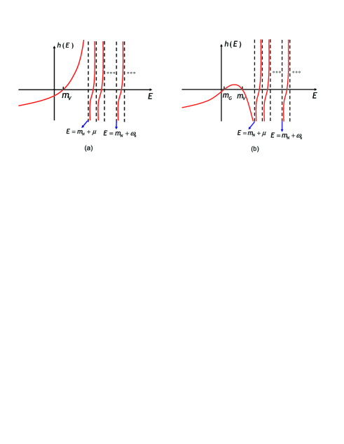
Figure 1: (Color online) The schematic for the function $h(E)$: the red curves denote the function $h(E)$, and the solutions $E=m_{N}+\omega_{k}$ are the energy of the scattering states, (a) when $g<g_{c}$, the equation $h(E)=0$ possesses only one real root $E=m_{V}$ in the regime $E<m_{N}+\omega_{k}$ when $h(m_{N}+\mu)>0$; (b) when $g>g_{c}$, the equation $h(E)=0$ possesses two real roots $E=m_{V}$ and $E=m_{G}$ in the regime $E<m_{N}+\omega_{k}$ when $m_{0}<m_{N}+\mu$.

We find physical $V$-state with $E=m_{V}$ in the regime $m_{V}<m_{N}+\mu$ as

$$\left|\mathbf{V}\right\rangle=Z_{V}^{1/2}[V^{\dagger}+\sum_{p}\phi_{V}(p)N^{\dagger}a_{p}^{\dagger}]\left|0\right\rangle,$$ (8)

where the momentum representation of wave-function is

$$\phi_{V}(p)=\frac{g_{0}f_{p}}{\sqrt{2\omega_{p}\Omega}}\frac{1}{m_{V}-m_{N}-\omega_{p}},$$ (9)

and the normalization constant is

$$Z_{V}^{-1}=1+\sum_{p}\phi_{V}^{2}(p).$$ (10)

When $g_{0}\rightarrow 0$, the eigenstate $\left|\mathbf{V}\right\rangle$ becomes $V^{\dagger}\left|0\right\rangle$. Thus, the dressed state $\left|\mathbf{V}\right\rangle$ describes the renormalized $V$-particle, or called the physical $V$-particle. The physical mass of the $V$-particle is $m_{V}$, which satisfies $h(m_{V})=0$.

Next, we consider the scattering states

$$\left|\mathbf{N\theta}_{k}\right\rangle_{\pm}=[c_{k,\pm}V^{\dagger}+\sum_{p}\phi_{k,\pm}(p)N^{\dagger}a_{p}^{\dagger}]\left|0\right\rangle,$$ (11)

to satisfy $h(E=E_{k})=0$ for $E_{k}=m_{N}+\omega_{k}$. While we assume

$$c_{k,\pm}=g_{0}f_{k}h^{-1}(m_{N}+\omega_{k}\pm i0^{+})/\sqrt{2\omega_{k}\Omega},$$ (12)

the scattering features are reflected by the $\delta$-function in the wave-function

$$\phi_{k,\pm}(p)=\delta(k-p)+\frac{g_{0}f_{p}c_{k,\pm}}{\sqrt{2\omega_{p}\Omega}}\frac{1}{\omega_{k}-\omega_{p}\pm i0^{+}}.$$ (13)

The positive infinitesimal $0^{+}$ is introduced here such that the eigenstates (11) are rewritten as the standard Lippmann- Schwinger scattering states

$$\left|\mathbf{N\theta}_{k}\right\rangle_{\pm} = (1+\frac{1}{E_{k}-H\pm i0^{+}}H_{I})N^{\dagger}a_{k}^{\dagger}\left|0\right\rangle,$$

$$= N^{\dagger}a_{k}^{\dagger}\left|0\right\rangle+\frac{1}{E_{k}-H_{0}\pm i0^{+}}H_{I}\left|\mathbf{N\theta}_{k}\right\rangle_{\pm}.$$

Obviously, the eigenstates (11) as well as Eq. (II.1) describe the scattering of the $\theta$-particle with momentum $k$ by the $N$-particle. The corresponding $S$-matrix element

$$S_{pk}=\,_{-}\left\langle\mathbf{N\theta}_{p}\left|\mathbf{N\theta}_{k}\right\rangle_{+}\right.=e^{2i\delta_{k}}\delta_{kp},$$ (15)

is determined by the scattering phase shift $\delta_{k}=\arctan\beta_{k}$, where

$$\beta_{k}=\frac{g_{0}^{2}Z_{V}k}{4\pi(m_{V}-m_{N}-\omega_{k})}[1-\frac{g_{0}^{2}Z_{V}}{(2\pi)^{3}}\Theta_{k}]^{-1},$$ (16)

and

$$\Theta_{k}=\mathcal{P}\int\frac{d^{3}p(m_{V}-m_{N}-\omega_{k})}{2\omega_{p}(\omega_{p}-\omega_{k})(m_{V}-m_{N}-\omega_{p})^{2}}.$$ (17)

Here, $\mathcal{P}$ denotes the principal-value integral. Because $Z_{V}^{-1}$ in Eq. (10) contains the divergent integral $\sum_{p}\phi_{V}^{2}(p)$ when the cutoff tends to infinite, i.e., $f_{p}\rightarrow 1$, the normalization constant $Z_{V}$ tends to zero so that the phase shift $\delta_{k}$ and the cross section both vanish. For avoiding the vanishing of the cross section, we introduce the physical coupling constant $g^{2}=g_{0}^{2}Z_{V}$ and assigne it to be finite.

II.2 Breaking of Unitarity and Emerging Ghost State

The normalization constant can be rewritten as

$$Z_{V}=1-\frac{g^{2}}{g_{c}^{2}},$$ (18)

in terms of the critical coupling constant $g_{c}^{2}$ defined as

$$g_{c}^{-2}=\sum_{p}\frac{f_{p}^{2}}{2\omega_{p}\Omega}\frac{1}{(m_{V}-m_{N}-\omega_{p})^{2}}.$$ (19)

Then the relation between $g^{2}$ and $g_{0}^{2}$ is

$$g_{0}^{2}=\frac{g^{2}g_{c}^{2}}{g_{c}^{2}-g^{2}}\text{.}$$ (20)

Obviously, if $g^{2}<g_{c}^{2}$, the normalization constant $Z_{V}$ and the square $g_{0}^{2}$ of the bare coupling constant are always positive, so that the conventional approach based on QFT is self-consistent and proper. However, if $g^{2}>g_{c}^{2}$, the normalization constant is negative, namely, the physical $V$-state has the negative norm. In addition, the square $g_{0}^{2}$ of bare coupling constant becomes negative, so that $g_{0}=i\lambda_{0}$ ($\lambda_{0}\in$ real number) is imaginary, which results in that the Lee model Hamiltonian is not Hermitian with respect to the conventional inner product and the unitarity is broken.

As illustrated in Fig. 1b, when $g_{0}$ is imaginary, the detail analysis shows that when $m_{0}>m_{N}+\mu$, there is no real solution satisfied $E<m_{N}+\mu$, but when $m_{0}<m_{N}+\mu$ there are two real solutions satisfied $E<m_{N}+\mu$. In this paper, we consider the case $m_{0}<m_{N}+\mu$ and prove that if $g_{0}$ is imaginary, the secular equation $h(E)=0$ possesses another real solution $E=m_{G}$ ($<m_{V}$) in the regime $E<m_{N}+\mu$ besides the real root $E=m_{V}$.

To consider the physics of this solution we rewrite $h(E)$ as $h(E)=Z_{V}^{-1}(E-m_{V})F(E)$, where

$$F(E)=1-\frac{g^{2}}{(2\pi)^{3}}\int\frac{d^{3}p(E-m_{V})}{2\omega_{p}\Lambda(E,\omega_{p})\Lambda^{2}(m_{V},\omega_{p})}.$$ (21)

and $\Lambda(E,\omega_{p})=E-m_{N}-\omega_{p}$. The schematics of the functions $h(E)$ and $F(E)$ are shown in Fig. 1a (b) and Fig. 2a (b) for the case $g>g_{c}$ ($g<g_{c}$), which display the relations $\partial_{E}F(E)>0$ and $F(m_{V})=1$ explicitly.

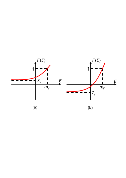
Figure 2: (Color online) The schematic for the function $F(E)$: the red curves denote the function $F(E)$, (a) when $g<g_{c}$, the equation $F(E)=0$ possesses no root in the regime $E<m_{N}+\omega_{k}$; (b) when $g>g_{c}$, the equation $F(E)=0$ possesses one real root $E=m_{G}$ in the regime $E<m_{N}+\omega_{k}$.

It is remarkable that as $E\rightarrow-\infty$, $F(E)\rightarrow Z_{V}$. Then we conclude that if $g>g_{c}$, i.e., $Z_{V}<0$, there always exists the real root $m_{G}$ of equation $h(E)$ in the interval $(-\infty,m_{V})$ when $m_{0}<m_{N}+\mu$, which is the energy of the ghost state. Here, the un-normalized ghost state is

$$\left|\mathbf{G}\right\rangle=[V^{\dagger}+\sum_{p}\phi_{G}(p)N^{\dagger}a_{p}^{\dagger}]\left|0\right\rangle,$$ (22)

where wave-function in the momentum representation is

$$\phi_{G}(p)=\frac{g_{0}f_{p}}{\sqrt{2\omega_{p}\Omega}}\frac{1}{m_{G}-m_{N}-\omega_{p}}.$$ (23)

The energy spectrums of the Lee model in the $V/N\theta$ sector are displayed in Fig. 3 schematically for the case $g>g_{c}$ and $g<g_{c}$.

To overcome the difficulty of negative norm when $g>g_{c}$, the metric $\zeta=(-1)^{n_{V}}$ is introduced by Källen and Pauli Pauli ; LW1 ; LW2 . They found that for the case $g>g_{c}$, in the new inner product space the norms $\left\langle\mathbf{V}\right|\zeta\left|\mathbf{V}\right\rangle$ and ${}_{\pm}\left\langle\mathbf{N\theta}_{k}\right|\zeta\left|\mathbf{N\theta}_{k}\right\rangle_{\pm}$ were both positive, and the orthogonal relations ${}_{\pm}\left\langle\mathbf{N\theta}_{k}\right|\zeta\left|\mathbf{V}\right\rangle=\left\langle\mathbf{V}\right|\zeta\left|\mathbf{N\theta}_{k}\right\rangle_{\pm}=0$ were also ensured. However, the norm $\left\langle\mathbf{G}\right|\zeta\left|\mathbf{G}\right\rangle$ of the ghost state was still negative and thus the ghost state phenomenon still exists! The negative norm of the ghost state implies that the metric $\zeta$ is an indefinite metric, and the $S$-matrix satisfies $\zeta S^{\dagger}\zeta S=1$, which is non-unitary. Recently, Bender et al. Bender introduced the different inner product by the $\mathcal{CPT}$ symmetry to insure the positive norms of the all eigenstates in the sector $V/N\theta$ for $g>g_{c}$. In this paper, we use the standard bi-orthogonal basis approach to find the proper inner product that automatically ensures the orthogonality and the positive definite of the eigenstates.

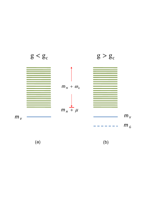
Figure 3: (Color online) The schematic for the energy spectrum in the $V/N\theta$ sector: when $g>g_{c}$, the ghost state emerges as a discrete state labelled by $m_{G}$. The discrete state labelled by $m_{V}$ is the physical $V$-state. Here, $m_{N}+\omega_{k}$ denotes the energy of the scattering state. $m_{V}$ and $m_{G}$ denote the energies of the physical $V$-particle state and ghost state.

III Bi-orthogonal basis used for one boson mode Lee model

In this section, we first briefly introduce the key ideas of the bi-orthogonal basis with its application to the one boson Lee model (or called QM Lee model) where the $\theta$-particle only has one mode, which has been studied extensively Bender ; Jones ; Trubatch .

III.1 Bi-orthogonal basis approach and Metric operator

In the bi-orthogonal basis approach to the non-Hermitian Hamiltonian $H$, the eigenstates and the corresponding eigenvalues $\left|e_{n}\right\rangle$ and $E_{n}$ determined by the eigen-equation $H\left|e_{n}\right\rangle=E_{n}\left|e_{n}\right\rangle$ can span the whole Hilbert space in some sense, but arbitrary two eigenstates are usually not orthogonal to each other. To have a complete orthogonal basis, we need the eigenstates $\left|d_{m}\right\rangle$ of $H^{\dagger}$ with corresponding eigenvalues $E_{m}^{D}$. Then we have the two sets of the basis {$\left|e_{n}\right\rangle$} and {$\left|d_{m}\right\rangle$}, and we can prove that if $E_{m}^{D}\neq E_{n}^{\ast}$ $\left\langle d_{m}\left|e_{n}\right\rangle\right.=0$, and if $E_{m}^{D}=E_{n}^{\ast}$ $\left\langle d_{m}\left|e_{n}\right\rangle\right.$ is nonzero. Hereafter, we define $\left|d_{n}\right\rangle$ is the eigenstate with the eigenvalue $E_{n}^{\ast}$ of the Hamiltonian $H^{\dagger}$ and do not assume their normalization. The two sets of the basis {$\left|e_{n}\right\rangle$} and {$\left|d_{n}\right\rangle$} form the so-called bi-orthogonal basis Sun ; Bi-O .

With the help of bi-orthogonal basis, the completeness relation is

$$\sum_{n}\frac{\left|e_{n}\right\rangle\left\langle d_{n}\right|}{\left\langle d_{n}\left|e_{n}\right\rangle\right.}=\sum_{n}\frac{\left|d_{n}\right\rangle\left\langle e_{n}\right|}{\left\langle e_{n}\left|d_{n}\right\rangle\right.}=1.$$ (24)

If we define the normalized basis by $\left|E_{n}\right\rangle=\left|e_{n}\right\rangle/\sqrt{\left\langle d_{n}\left|e_{n}\right\rangle\right.}$ and $\left|d_{n}\right\rangle=\left|d_{n}\right\rangle/\sqrt{\left\langle e_{n}\left|d_{n}\right\rangle\right.}$, we have the generic completeness relations

$$\sum|E_{n}\rangle\langle D_{n}|=\sum|D_{n}\rangle\langle E_{n}|=1,$$ (25)

and

$$\langle D_{n}|E_{m}\rangle=\langle E_{n}|D_{m}\rangle=\delta_{mn}.$$ (26)

According to Refs. Bi-O , we can define the new inner product

$$(\Phi,\Psi)=\left\langle\Phi^{D}\left|\Psi\right\rangle=\left\langle\Phi\right|\eta\left|\Psi\right\rangle\right.,$$ (27)

with new metric operator $\eta$:

$$|E_{n}\rangle\rightarrow|D_{n}\rangle=\eta|E_{n}\rangle.$$ (28)

The Hamiltonian $H$ under the new metric is Hermitian, i.e., $\eta H=H^{\dagger}\eta$ or $(\Phi,H\Psi)^{\ast}=(\Psi,H\Phi)$. Thus, for the non-Hermitian Hamiltonian that satisfies $\eta H=H^{\dagger}\eta$, we always find out the metric $\eta$ by bi-orthogonal basis, so that in the new inner product space the Hamiltonian becomes Hermitian and the all eigenstates have the positive norms, and the arbitrary two eigenstates are orthogonal to each other.

III.2 One boson mode Lee model

In this subsection, we use the bi-orthogonal basis to deal with the simple model, i.e., one boson mode Lee model or called QM Lee model. To show the main ideas to solve the unitarity problem of the standard Lee model (the QFT Lee Model), we first consider the one boson mode Lee model, namely, the $\theta$-particle only has one mode, which has been studied extensively Bender ; Jones ; Trubatch . It can be proved that this model is equivalent to the “standard model” of quantum optics, the Jaynes-Cummings (JC) model JC (see the appendix).

The one boson mode Lee model is described by the Hamiltonian $H_{s}=H_{0}+H_{1}$, where

$$H_{0}=m_{0}V^{\dagger}V+m_{N}N^{\dagger}N+\varepsilon a^{\dagger}a,$$ (29)

and

$$H_{1}=g_{0}(aV^{\dagger}N+h.c.).$$ (30)

When $g_{0}=i\lambda_{0}$ is imaginary, we use the bi-orthogonal basis approach to reconsider the Hermiticity of $H_{s}$. The eigenstates of the Hamiltonian $H_{s}$ in the subspace spanned by the basis $V^{\dagger}\left|0\right\rangle$ and $N^{\dagger}a^{\dagger}\left|0\right\rangle$ are

$$\left|\Psi_{\pm}\right\rangle=\mathcal{N}_{\pm}^{-1}[i\lambda_{0}V^{\dagger}+(E_{\pm}-m_{0})N^{\dagger}a^{\dagger}]\left|0\right\rangle,$$ (31)

and the corresponding eigenvalues are

$$E_{\pm}=\frac{1}{2}(s\pm\sqrt{u^{2}-4\lambda_{0}^{2}}),$$ (32)

where the normalization constants $\mathcal{N}_{\pm}$ are determined below. Here, $s=m_{N}+\varepsilon+m_{0}$ and $u=m_{N}+\varepsilon-m_{0}$. Obviously, the eigenvalues are all real only if $u^{2}-4\lambda_{0}^{2}>0$. Here, we focus on the case $u^{2}-4\lambda_{0}^{2}>0$ so that all energies are real in this sector. Below we only consider the case $u>2\lambda_{0}$, and the other case $u<-2\lambda_{0}$ can be discussed in the similar manner.

It is clear that with respect to the conventional inner product $\left\langle\Phi\left|\Psi\right\rangle\right.$ the two eigenstates are not orthogonal to each other, i.e., $\left\langle\Psi_{\mp}\left|\Psi_{\pm}\right\rangle\right.\neq 0$, and the normalization constants are

$$\mathcal{N}_{\pm,\mathrm{old}}^{2}=u(E_{\pm}-m_{0}),$$ (33)

where the subscript “$\mathrm{old}$” denotes the normalization constants are defined in the conventional inner product space. In the dual representation the eigenstates of the conjugate Hamiltonian $H_{s}^{\dagger}=H_{0}-H_{1}$ are

$$\left|\Psi_{\pm}^{D}\right\rangle=\pm\mathcal{N}_{\pm}^{-1}[-i\lambda_{0}V^{\dagger}+(E_{\pm}-m_{0})N^{\dagger}a^{\dagger}]\left|0\right\rangle,$$ (34)

with the corresponding eigenvalues $E_{\pm}^{D}=E_{\pm}$. It can be verified that $\left.\left\langle\Psi_{+}^{D}\right|\Psi_{-}\right\rangle=\left.\left\langle\Psi_{-}^{D}\right|\Psi_{+}\right\rangle=0$, and $\left.\left\langle\Psi_{\pm}^{D}\right|\Psi_{\pm}\right\rangle\neq 0$.

To overcome the non-orthogonality difficulty, we find out the new metric

$$\eta=\left|\Psi_{+}^{D}\right\rangle\left\langle\Psi_{+}^{D}\right|+\left|\Psi_{-}^{D}\right\rangle\left\langle\Psi_{-}^{D}\right|,$$ (35)

or its explicit form in operators:

$$\eta = \frac{1}{\sqrt{u^{2}-4\lambda_{0}^{2}}}[u(V^{\dagger}V+N^{\dagger}N)$$ (36)

$$-2i\lambda_{0}(V^{\dagger}Na-h.c.)],$$

by solving the equation $\left|\Psi_{\pm}^{D}\right\rangle=\eta\left|\Psi_{\pm}\right\rangle$. Then we define the new inner product $(\Phi,\Psi)=\left\langle\Phi\right|\eta\left|\Psi\right\rangle=\left\langle\Phi^{D}\right|\Psi\rangle=\left\langle\Phi\right|\Psi^{D}\rangle$: $|\Psi^{D}\rangle=\eta\left|\Psi\right\rangle$ in the single particle subspace. The orthogonality $\left.\left\langle\Psi_{+}^{D}\right|\Psi_{-}\right\rangle=\left.\left\langle\Psi_{-}^{D}\right|\Psi_{+}\right\rangle=0$ and the positively definite norm of the eigenstates are both ensured in the new inner product space defined by metric $\eta$. And the Hamiltonian is also Hermitian, i.e., $\eta H=H^{\dagger}\eta$. The new normalization condition $\left.\left\langle\Psi_{+}^{D}\right|\Psi_{+}\right\rangle=\left.\left\langle\Psi_{-}^{D}\right|\Psi_{-}\right\rangle=1$ gives

$$\mathcal{N}_{\pm}^{2}=\sqrt{u^{2}-4\lambda_{0}^{2}}(E_{\pm}-m_{0})>0,$$ (37)

which are different from the normalization constants (33) determined by the conventional inner product. Then we also have the completeness relation

$$\eta(\left|\Psi_{+}\right\rangle\left\langle\Psi_{+}\right|+\left|\Psi_{-}\right\rangle\left\langle\Psi_{-}\right|) = 1,$$ (38)

$$(\left|\Psi_{+}\right\rangle\left\langle\Psi_{+}\right|+\left|\Psi_{-}\right\rangle\left\langle\Psi_{-}\right|)\eta = 1.$$ (39)

IV Lee model with $g>g_{c}$

In this section, we study the QFT Lee model by using the bi-orthogonal basis approach. The problem is considered in the subspace with $n_{\theta}+n_{V}=1$ when the bare coupling constant $g_{0}=i\lambda_{0}$ ($\lambda_{0}\in R$) is imaginary, i.e., $g>g_{c}$. We will prove in the appendix that the QFT Lee model is essentially a massive JC model where the “light field” would be massive.

We first consider the ghost state and physical $V$-state. We show that in the new inner product space, the ghost state and physical $V$-state have positive norms. Secondly, we consider the scattering states of the $\theta$-particle. We prove that the scattering states also have positive norms in the new inner product space.

Let me first present the new metric operator

$$\eta = bV^{\dagger}V+\sum_{kp}W_{kp}N^{\dagger}Na_{k}^{\dagger}a_{p}$$ (40)

$$+\sum_{k}(s_{k}V^{\dagger}Na_{k}+h.c.),$$

for the Lee model as our central result. Here, the parameters $b=2\Xi_{G}-1$ and $s_{p}=2\Xi_{G}\phi_{G}(p)$ are defined by

$$\Xi_{G}^{-1} = 1+\sum_{p}\phi_{G}^{2}(p),$$ (41)

$$W_{kp} = \delta_{kp}-2\Xi_{G}\phi_{G}(k)\phi_{G}(p).$$ (42)

It will be proved soon as follows that the inner product $(\Phi,\Psi)=\left\langle\Phi\right|\eta\left|\Psi\right\rangle$ based on this metric will solve all the problems in the Lee model with $g>g_{c}$: (1) the ghost state and physical $V$-state have positive norms; (2) the scattering states of the $\theta$-particle has the positive norms; (3) the orthogonality of the eigenstates is ensured; (4) the unitarity of the $S$-matrix for the $N\theta\rightarrow N\theta$ process is recovered automatically.

IV.1 Ghost state and physical $V$-state

The energies of the ghost state and physical $V$-state are located out of the continuum, i.e., $m_{L}-m_{N}-\omega_{k}<0$ for $L=\mathbf{V}$ and $\mathbf{G}$. In this case, the ghost state and physical $V$-state are expressed as an unified form

$$\left|L\right\rangle=\Xi_{L}^{1/2}[V^{\dagger}+\sum_{p}\phi_{L}(p)N^{\dagger}a_{p}^{\dagger}]\left|0\right\rangle.$$ (43)

Here, the normalized constants $\Xi_{L}$ are determined by the bi-orthogonal basis approach below. To find out the proper inner product, we consider that two dual eigenstates

$$\left|\mathbf{V}^{D}\right\rangle = \Xi_{V}^{1/2}[-V^{\dagger}+\sum_{p}\phi_{V}(p)N^{\dagger}a_{p}^{\dagger}]\left|0\right\rangle,$$

$$\left|\mathbf{G}^{D}\right\rangle = \Xi_{G}^{1/2}[V^{\dagger}-\sum_{p}\phi_{G}(p)N^{\dagger}a_{p}^{\dagger}]\left|0\right\rangle,$$ (44)

of $H^{\dagger}$ have the same eigenvalues $m_{L}$. Then we define the inner products $(\mathbf{V},\mathbf{V})=\left\langle\mathbf{V}^{D}\left|\mathbf{V}\right\rangle\right.$, $(\mathbf{G},\mathbf{G})=\left\langle\mathbf{G}^{D}\left|\mathbf{G}\right\rangle\right.$, $(\mathbf{V},\mathbf{G})=\left\langle\mathbf{V}^{D}\left|\mathbf{G}\right\rangle\right.$ and $(\mathbf{G},\mathbf{V})=\left\langle\mathbf{G}^{D}\left|\mathbf{V}\right\rangle\right.$ for the ghost state and physical $V$-state. The normalization conditions $\left\langle\mathbf{V}^{D}\left|\mathbf{V}\right\rangle\right.=\left\langle\mathbf{G}^{D}\left|\mathbf{G}\right\rangle\right.=1$ lead to the constants $\Xi_{G}^{-1}$ in Eq. (41) and

$$\Xi_{V}=\frac{g^{2}}{g_{c}}-1>0.$$ (45)

Obviously, with respect to the new inner products, the conditions $(\mathbf{V},\mathbf{V})=(\mathbf{G},\mathbf{G})=1$ and $(\mathbf{V},\mathbf{G})=(\mathbf{G},\mathbf{V})=0$ are satisfied simultaneously.

IV.2 Scattering states and unitarity of the $S$-matrix

The energies of the scattering states are $E_{k}=m_{N}+\omega_{k}$. The corresponding eigenstates of Hamiltonian $H$ are $\left|\mathbf{N\theta}_{k}\right\rangle_{\pm}$. In the dual space, the corresponding eigenstates

$$\left|\mathbf{N\theta}_{k}^{D}\right\rangle_{\pm}=[-c_{k,\pm}V^{\dagger}+\sum_{p}\phi_{k,\pm}(p)N^{\dagger}a_{p}^{\dagger}]\left|0\right\rangle,$$ (46)

of Hamiltonian $H^{\dagger}$ have the same eigenvalues $E_{k}=m_{N}+\omega_{k}$. The eigenstates (46) are rewritten as

$$\left|\mathbf{N\theta}_{k}^{D}\right\rangle_{\pm}=N^{\dagger}a_{k}^{\dagger}\left|0\right\rangle+\frac{1}{E_{k}-H_{0}\pm i0^{+}}H_{I}^{\dagger}\left|\mathbf{N\theta}_{k}^{D}\right\rangle_{\pm}\,,$$ (47)

which are the standard form of the Lippmann-Schwinger represntation. Obviously, the eigenstates (II.1), (43), (44), and (47) immediately give the orthogonal relations

$${}_{\pm}\left\langle\mathbf{N\theta}_{k}^{D}\left|\mathbf{N\theta}_{p}\right\rangle_{\pm}\right. = \,{}_{\pm}\left\langle\mathbf{N\theta}_{p}\left|\mathbf{N\theta}_{k}^{D}\right\rangle_{\pm}\right.=\delta_{kp},$$

$$\left\langle\mathbf{V}^{D}\left|\mathbf{N\theta}_{p}\right\rangle_{\pm}\right. = \,{}_{\pm}\left\langle\mathbf{N\theta}_{p}^{D}\left|\mathbf{V}\right\rangle\right.=0.$$ (48)

With the help of the eigenstates of the Hamiltonian $H$ and the dual Hamiltonian $H^{\dagger}$, we find the new metric $\eta$, which is satisfies $\eta\left|\Psi\right\rangle=\left|\Psi^{D}\right\rangle$, so that the inner product is $(\Phi,\Psi)=\left\langle\Phi\right|\eta\left|\Psi\right\rangle$. For the eigenstates, the relations $\eta\left|\mathbf{V}\right\rangle=\left|\mathbf{V}^{D}\right\rangle$, $\eta\left|\mathbf{G}\right\rangle=\left|\mathbf{G}^{D}\right\rangle$, and $\eta\left|\mathbf{N\theta}_{k}\right\rangle_{\pm}=\left|\mathbf{N\theta}_{k}^{D}\right\rangle_{\pm}$ immediately result in the metric (40). Under this proper metric, in this subspace all states always have the positive norms, and the arbitrary two eigenstates are orthogonal to each other. And the Hamiltonian satisfies $\eta H=H^{\dagger}\eta$, which implies the Hamiltonian is Hermitian under the new metric.

Under the new metric, the $S$-matrix elements are defined by

$$S_{pk}=\,_{-}\left\langle\mathbf{N\theta}_{p}\right|\eta\left|\mathbf{N\theta}_{k}\right\rangle_{+}=\,_{-}\left\langle\mathbf{N\theta}_{p}^{D}\left|\mathbf{N\theta}_{k}\right\rangle_{+}\right..$$ (49)

The Lippmann-Schwinger formalism results in the $S$-matrix elements as

$$S_{pk}=\delta_{kp}-2\pi i\delta(E_{k}-E_{p})T_{pk},$$ (50)

where

$$T_{pk}=\frac{g_{0}f_{p}\left\langle 0\right|V\left|\mathbf{N\theta}_{k}\right\rangle_{+}}{\sqrt{2\omega_{p}\Omega}}=\frac{g_{0}f_{p}c_{k,+}}{\sqrt{2\omega_{p}\Omega}},$$ (51)

defines the transfer matrix, i.e., $T$-matrix, and the $S$-matrix element is obtained as $S_{pk}=\delta_{kp}\exp(2i\delta_{k})$, where the phase shift $\delta_{k}=\arctan\beta_{k}$ as $f_{k}\rightarrow 1$. Obviously, the $S$-matrix is unitary under the new metric. It is shown that the choice of the above matric indeed does not the representation of the $S$-matrix and thus the physically observable result remains the same as that in the conventional matric.

V Conclusion

Finally, let us briefly summarize our results as follows. For one boson mode Lee model with an imaginary coupling constant, the Hamiltonian is non-Hermitian with respect to the inner product defined in the conventional QM, but we can use bi-orthogonal basis to find a proper inner product , so that the Hamiltonian becomes Hermitian with respect to the new inner product. This inner product insures the orthogonality and the positive definiteness of norm of eigenstates. For the QFT Lee model with $g>g_{c}$, the Hamiltonian is also non-Hermitian in the inner product defined in the conventional QFT. Based on the bi-orthogonal basis approach the proper inner product is also found. The proper inner product automatically insures the Hermiticity of the Hamiltonian, the orthogonality and the positive definite norms of the eigenstates. Physically the ghost state is killed in our approach so that the unitarity of the $S$-matrix is recovered automatically.

Since the Lee model was found in 1954, there were many struggles to find the proper metric so that the positive definite norms of the eigenstates were insured. We have pointed out that the inner product introduced by Pauli et al. Pauli did not insure the positive norm of the ghost state. Our inner product is so proper that the orthogonality and the positive definite norms of the eigenstates are ensured simultaneously. And the Hamiltonian becomes Hermitian in the Hilbert space with the new metric, which ensures the unitary evolution of the quantum states. Our investigations about the Lee model suggest that the Hermiticity of the Hamiltonian is related to the definition of the inner product space though this point is very clear in mathematics. For the non-Hermitian Hamiltonian in one inner product space with the metric, it may become Hermitian in another inner product space with the different metric.

In the future work, we will used the bi-orthogonal basis to reconsider the unitarity of the $S$-matrix in the higher sectors, such as $N\theta\theta$ sector Pauli ; LW2 ; NTT1 ; NTT2 ; NTT3 ; NTT4 . We would establish the new theoretical system of QFT by the bi-orthogonal basis, such as the new Feynman rules, renormalization procedure LW1 and reduction formalism LSZ ; LSZ1 ; LSZ2 . The bi-orthogonal basis can also be used to reconsider the strong-coupling induced unitarity problem for the generalized Lee Model in quantum optics Zhou1 ; FanPRL ; FanPRA ; Zhou ; Shi ; Xu , atom physics F ; Xu , condensed matter physics A and the high energy physics neutron ; LQCD .

*

Appendix A Relationship between Lee mode and a “Standard model” in quantum optics

The JC models with one mode and multi-modes can be regarded as a “standard model” in quantum optics or cavity QED, which deals with the discrete levels interacting with some continuum L ; S . In the appendix, we consider the relation between the Lee model and the multi-mode JC model with the Hamiltonian

$$H_{\mathrm{sb}} = \Omega\left|e\right\rangle\left\langle e\right|+\sum_{k}\omega_{k}a_{k}^{\dagger}a_{k}$$ (52)

$$+\sum_{k}G_{k}(a_{k}\left|e\right\rangle\left\langle g\right|+h.c.),$$

where $\left|e\right\rangle$ and $\left|g\right\rangle$ are the excited and ground states of a two level atom with energy level spacing $\Omega$. Here, $a_{k}$ ($a_{k}^{\dagger}$) denotes the annihilation (creation) operator of the photon with dispersion relation $\omega_{k}=k=\sqrt{k_{x}^{2}+k_{y}^{2}+k_{z}^{2}}$. The coupling

$$G_{k}^{2}=\frac{\omega_{k}}{2\epsilon_{0}(2\pi)^{3}}D^{2}\cos^{2}\varphi_{k},$$

of the atom to photon is determined by the angle $\varphi_{k}$ between the atomic dipole momentum $D$ and the electric field polarization vector of photon, where $\epsilon_{0}$ is dielectric constant in vacuum.

This model can be applied to describe the spontaneous emission of the atom. In the single mode limit, the model becomes the single mode JC model

$$H_{\mathrm{JC}} = \Omega\left|e\right\rangle\left\langle e\right|+\omega_{0}a^{\dagger}a$$ (53)

$$+G_{0}(a\left|e\right\rangle\left\langle g\right|+h.c.),$$

which is just the one boson mode Lee model or QM Lee model discussed in Sec. III.

Comparing Eq. (52) with the Lee model, we find that the multi-mode JC model is formally the massless Lee model with $m_{N}=0$, $\mu=0$, $\Omega=m_{0}$, and $G_{k}=g_{0}f_{k}/\sqrt{2\omega_{k}\Omega}$. However, the Lee model has very different nature from that of the multi-mode JC model due to the non-vanishing mass $\mu$. Thus, owing to the different dispersion relation, the Lee model may has the stable $V$-particle state $\left|\mathbf{V}\right\rangle$, but the multi-mode JC model possess the unstable excited state that has the finite lifetime and decays to the ground state by emitting photon.

In the following discussions, we calculate the lifetime of the excited state of the two level atom by the scattering theory. Now, we do not limit the form of the dispersion relation $\omega_{k}=w(k)$, but we assign it with a lower cutoff $\omega_{\min}$ for any $k$. In this sense, we can generally study how the form of dispersion relation effects on the existence of the bound states.

We consider the scattering states

$$\left|g,k\right\rangle_{\pm}=u_{k,\pm}\left|e\right\rangle+\sum_{p}\chi_{k,\pm}(p)a_{p}^{\dagger}\left|g\right\rangle,$$ (54)

corresponding to $\left|\mathbf{N}\theta_{k}\right\rangle_{\pm}$ in the Lee model. Here,

$$u_{k,\pm} = G_{k}h_{sb,\pm}^{-1}(\omega_{k}),$$

$$\chi_{k,\pm}(p) = \delta_{kp}+\frac{G_{p}u_{k,\pm}}{\omega_{k}-\omega_{p}\pm i0^{+}},$$ (55)

are determined by the eigen-equation $H_{\mathrm{sb}}\left|g,k\right\rangle_{\pm}=\omega_{k}\left|g,k\right\rangle_{\pm}$. We define the function $h_{sb,\pm}(\omega)=\mathbf{G}_{\pm}^{-1}(\omega)$, where

$$\mathbf{G}_{\pm}(\omega)=[\omega-\Omega-\sum_{p}\frac{G_{p}^{2}}{\omega-\omega_{p}\pm i0^{+}}]^{-1},$$ (56)

is just the retarded $\mathbf{G}_{+}(\omega)$ or advanced $\mathbf{G}_{-}(\omega)$ Green’s function of the excited state. Then the $S$-matrix elements $S_{kp}=$ ${}_{-}\left\langle N\theta_{p}\left|N\theta_{k}\right\rangle_{+}\right.$ are

$$S_{kp}=\delta_{kp}-2\pi i\delta(\omega_{k}-\omega_{p})G_{k}u_{k,+},$$ (57)

and thus the scattering phase shift is

$$e^{2i\delta_{k}}=\frac{\mathbf{G}_{sb,+}(\omega_{k})}{\mathbf{G}_{sb,+}^{\ast}(\omega_{k})}\text{.}$$ (58)

If there existed the bound states

$$\left|B\right\rangle=\left|e\right\rangle+\sum_{p}\chi_{B}(p)a_{p}^{\dagger}\left|g\right\rangle,$$ (59)

in this system for $\chi_{B}(p)=G_{p}(E_{B}-\omega_{p})^{-1}$, the energies $E_{B}<\omega_{\min}$ of the bound states $\left|B\right\rangle$ would satisfy

$$h_{sb,\pm}(E_{B})=\text{Re}h_{sb,\pm}(E_{B})=0.$$ (60)

Thus, we conclude that the poles of the $S$-matrix (57) or phase shift (58) determine the bound state energies.

Using Eq. (60), we discuss the existence of the bound states. Because $\partial_{\omega}h_{sb}(\omega)>0$ and $h_{sb}(\omega\rightarrow-\infty)\rightarrow-\infty$, Eq. (60) possess the real roots $E_{B}$ in the regime $E_{B}<\omega_{\min}$ only if $h_{sb}(\omega_{\min}^{-})>0$, where $\omega_{\min}^{-}=\omega_{\min}-0^{+}$. However, in the opposite case $h_{sb}(\omega_{\min}^{-})<0$, i.e.,

$$\omega_{\min}^{-}+\int d^{3}p\frac{G_{p}^{2}}{\omega_{p}-\omega_{\min}^{-}}<\Omega,$$ (61)

there is no real root in the regime $E_{B}<\omega_{\min}$. In this case (61), Eq. (60) possess the imaginary solution $E_{\mathbf{quasi}}=E_{b}-i\gamma$ in the regime $E_{b}>\omega_{\min}$. Though the solution $E_{\mathbf{quasi}}$ is not the eigenvalue of the Hamiltonian due to the Hermiticity of the Hamiltonian, it describes the unstable excited state with the energy $E_{b}$ and the lifetime $1/\gamma$. For the small decay rate, the real part $E_{b}$ and the decay rate $\gamma$ are determined by

$$\text{Re}h_{sb,+}(E_{b})=0,$$ (62)

and

$$\gamma=\frac{\text{Im}h_{sb,+}(E_{b})}{\left.\partial_{\omega}\text{Re}h_{sb,\pm}(\omega)\right|_{\omega=E_{b}}},$$ (63)

approximately ZS . Here, Re$h_{sb,+}(E_{b})=$Re$h_{sb,-}(E_{b})$. On the other hand, near the pole $E_{\mathbf{quasi}}$ the Green’s function $\mathbf{G}_{+}(\omega)$ of the excited state is

$$\mathbf{G}_{+}(\omega) = \frac{1}{\text{Re}h_{sb,\pm}(E_{b})+i\text{Im}h_{sb,\pm}(E_{b})},$$ (64)

$$\sim \frac{Z}{\omega-E_{b}+i\gamma},$$

where $Z^{-1}=\left.\partial_{\omega}\text{Re}h_{sb,+}(\omega)\right|_{\omega=E_{b}}$. It is remarkable that when the energy of incident photon equals to $E_{b}$, the phase shift $\delta_{k}$ goes to $\pi/2$ so that the cross section tends to infinite, which exhibits a typical resonance.

In the Lee model, $\omega_{\min}$ regardes the mass $\mu$ of boson, so that under the condition $h(m_{N}+\mu)>0$ there always exists the bound state $\left|\mathbf{V}\right\rangle$, i.e., the physical $V$-particle state without the imaginary part of the eigen-energy. However, if $h(m_{N}+\mu)<0$ the bound state vanishes, and the stable $V$-particle state becomes the unstable state. Thus, we conclude that in the Lee model, due to the non-vanishing mass $\mu$, the system contains the bound state $\left|\mathbf{V}\right\rangle$ only if $h(m_{N}+\mu)>0$. The analytic property of the Green’s function $\mathbf{G}_{+}(\omega)$ in the whole complex-$\omega$ plane is shown in Fig. 4, which exhibits that when $h(m_{N}+\mu)<0$, the bound state vanishes and two poles $E_{\pm}$ in the upper and lower planes emerge, the imaginary part $\gamma$ of the $E_{+}$ is the decay rate of the unstable $V$-particle.

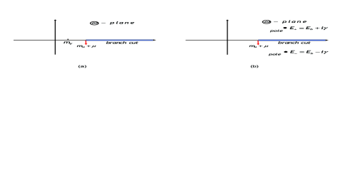
Figure 4: (Color online) The analytic property of the Green’s function $h^{-1}(\omega)$ of JC model as an Lee model with vanishing mass of $\theta$-particle: the Green’s function possesses the branch cut in the regime $\omega>m_{N}+\mu$, (a) if $h(m_{N}+\mu)>0$, the Green’s function has the pole $m_{V}$ corresponding to the bound state energy; (b) if $h(m_{N}+\mu)<0$, the bound state becomes the unstable $V$-particle and two poles $E_{\pm}$ in the upper and lower planes emerge, where $\gamma$ is the decay rate of the unstable $V$-particle LW1 .

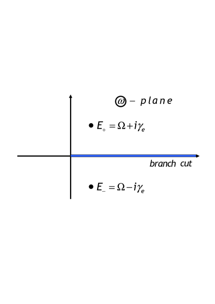
Figure 5: (Color online) The analytic property of the Green’s function $\mathbf{G}_{(}\omega)$: because the vanishing mass $\mu$, the excited state energy $\Omega$ is embedded in the continuum $\omega_{k}$ and the atom has the finite lifetime $1/\gamma_{e}$.

For the multi-mode JC model, the mass of the photon is zero. We except the excited state is greater than the ground state of the atom so that the energy of the excited state always locates in the continuum of the photon energy spectrum and the excited state is unstable with the lifetime $\tau\sim 1/\gamma_{e}$. The renormalized energy of excited-state is$\ \Omega_{r}=\Omega+\delta\Omega$, where the Lamb shift

$$\delta\Omega=\mathcal{P}\int d^{3}p\frac{G_{p}^{2}}{\Omega_{r}-\omega_{p}}.$$ (65)

is determined by the condition Re$h_{sb,+}(\omega)=0$. When Lamb shift is small, the decay rate of the excited state is

$$\gamma\sim\pi\sum_{p}G_{p}^{2}\delta(\Omega-\omega_{p})=\frac{\Omega^{3}D^{2}}{6\pi\epsilon_{0}},$$ (66)

which is just the spontaneous emission rate, which was given in many references L ; S ; ZS . The analytic property of the Green’s function

$$\mathbf{G}(\omega)=[\omega-\Omega-\sum_{p}\frac{G_{p}^{2}}{\omega-\omega_{p}}]^{-1},$$ (67)

in the whole complex-$\omega$ plane is shown in Fig. 5, which exhibits that the two poles $E_{\pm}$ in the upper and lower planes emerge and the imaginary part $\gamma$ of the $E_{+}$ is the spontaneous emission rate.

- (1) T. D. Lee, Phys. Rev. 95, 1329 (1954).
- (2) S. S. Schweber, An Introduction to Relativistic Quantum Field Theory (Row, Peterson and Co, Evanston, 1961), Chap. 12.
- (3) U. Fano, Phys. Rev. 124, 1866 (1961).
- (4) P. W. Anderson, Phys. Rev. 124, 41 (1961).
- (5) L. Zhou, F. M. Hu, J. Lu, and C. P. Sun, Phys. Rev. A, 74, 032102 (2006).
- (6) P. J. Redmond, Phys. Rev. 112, 1404 (1958).
- (7) G. Rasche and N. Straumann, Nuovo Cimento 4, 4604 (1962).
- (8) G. Källen and W. Pauli, Dan. Mat. -Fys. Medd. 30, 7 (1955).
- (9) T. D. Lee and G. C. Wick, Nucl. Phys. B 9, 209 (1969).
- (10) T. D. Lee and G. C. Wick, Nucl. Phys. B 10, 1 (1969).
- (11) C. M. Bender, S. F. Brandt, J. H. Chen, and Q. H. Wang, Phys. Rev. D 71, 025014 (2005).
- (12) H. F. Jones, Phys. Rev. D 77, 065023 (2008).
- (13) C. P. Sun, Phys. Scr. 48, 393 (1993).
- (14) P. T. Leung, W. M. Suen, C. P. Sun, and K. Young, Phys. Rev. E 57, 6101 (1998).
- (15) V. Glaser and G. Källen, Nucl. Phys. 2, 706 (1957).
- (16) S. L. Trubatch, Amer. J. Phys. 38, 331 (1970).
- (17) E. T. Jaynes and F. W. Cummings, Proc. IEEE 51, 89 (1963).
- (18) R. D. Amado, Phys. Rev. 122, 696 (1961).
- (19) A. Pagnamento, J. Math. Phys. 6, 955 (1965).
- (20) A. Pagnamento, J. Math. Phys. 7, 356 (1965).
- (21) E. M. Kazes, J. Math. Phys. 6, 1172 (1965).
- (22) H. Lehmann, K. Symanzik, and W. Zimmermann, Nuovo Cimento 1, 1425 (1955).
- (23) M. S. Maxon and R. B. Curtis, Phys. Rev. 137, B996 (1965).
- (24) M. S. Maxon, Phys. Rev. 149, 1273 (1966).
- (25) J. T. Shen and S. Fan, Phys. Rev. Lett. 98, 153003 (2007).
- (26) J. T. Shen and S. Fan, Phys. Rev. A 76, 062709 (2007).
- (27) L. Zhou, Z. R. Gong, Y. X. Liu, C. P. Sun and F. Nori, Phys. Rev. Lett. 101, 100501 (2008).
- (28) T. Shi and C. P. Sun, arXiv: quant-ph/0809.1279.
- (29) D. Z. Xu, H. Ian, T. Shi, H. Dong, and C. P. Sun, arXiv: quant-ph/0812.0429.
- (30) C. C. Nishi and M. M. Guzzo, Phys. Rev. D 78, 033008 (2008).
- (31) G. Z. Meng and C. Liu, Phys. Rev. D 78, 074506 (2008).
- (32) W. H. Louisell, Quantum Statistical Properties of Radiation (Wiley, NewYork, 1973).
- (33) M. O. Scully and M. S. Zubairy, Quantum Optics (Cambridge University Press 1997).
- (34) S. R. Zhao, C. P. Sun, and W. X. Zhang, Phys. Lett. A 207, 327 (1995).