Capacity of a Class of Symmetric SIMO Gaussian Interference Channels within $\mathcal{O}(1)$

Abstract

The $N+1$ user, $1\times N$ single input multiple output (SIMO) Gaussian interference channel where each transmitter has a single antenna and each receiver has $N$ antennas is studied. The symmetric capacity within $\mathcal{O}(1)$ is characterized for the symmetric case where all direct links have the same signal-to-noise ratio (SNR) and all undesired links have the same interference-to-noise ratio (INR). The gap to the exact capacity is a constant which is independent of SNR and INR. To get this result, we first generalize the deterministic interference channel introduced by El Gamal and Costa in [2] to model interference channels with multiple antennas. We derive the capacity region of this deterministic interference channel. Based on the insights provided by the deterministic channel, we characterize the generalized degrees of freedom (GDOF) of Gaussian case, which directly leads to the $\mathcal{O}(1)$ capacity approximation. On the achievability side, an interesting conclusion is that the generalized degrees of freedom (GDOF) regime where treating interference as noise is found to be optimal in the 2 user interference channel, does not appear in the $N+1$ user, $1\times N$ SIMO case. On the converse side, new multi-user outer bounds emerge out of this work that do not follow directly from the 2 user case. In addition to the GDOF region, the outer bounds identify a strong interference regime where the capacity region is established.

I Introduction

The capacity of the interference channel has been an open problem for over thirty years. The key to making progress on this problem is to pursue capacity approximations. Taking this approach, seminal work by Etkin, Tse and Wang [1] has produced the capacity characterization within one bit for the two user Gaussian interference channel. By further tightening one outer bound in [1], the sum capacity has been shown to be achievable by treating interference as noise in a very weak interference regime (also known as noisy interference regime) [3][4][5]. The succuss of this characterization follows from two important techniques, deterministic approach and generalized degrees of freedom. By focusing on the interaction between desired signals and interference, i.e., de-emphasizing local noise, the deterministic channels provide fundamental insights into their Gaussian counterparts [6][7]. The GDOF perspective, introduced in [1], presents a coarse, but insightful picture of the optimal achievable schemes and outer bounds for the interference channel. In particular, the GDOF picture for the symmetric case - which we refer to as the “W” curve- has come to represent the interference channel in the same way as the pentagonal capacity region is associated with the multiple access channel. The W curve delineates very weak, weak, moderate, strong and very strong interference regimes, each with a distinct character.

The next logical step is to extend these insights to interference networks - i.e., interference channels with more than 2 users. Extensions to more than 2 users have turned out to be non-trivial due to the emergence of some fundamentally new issues that are unique to interference networks. In particular, the idea of interference alignment is introduced in the context of interference networks by Cadambe and Jafar in [8] as the principal determinant of the network degrees of freedom (capacity pre-log). The extent to which interference can be aligned is very difficult to determine precisely in general. For this reason, even the exact capacity pre-log factor is unknown for almost all interference networks, including, e.g. the 3 user interference channel with constant channel coefficients[9][10]. Since the capacity pre-log dominates all other factors in a capacity approximation, most attempts to gain useful insights for interference networks get caught in the intricacies of interference alignment and do not make it past the degree-of-freedom question. Notable exceptions include the perfectly symmetric $K$ user interference channel considered in [11], and many-to-one (and one-to-many) interference channels considered in [7]. Jafar and Vishwanath [11] use interference alignment to show that the (per-user) GDOF characterization of the $K$ user interference channel in a perfectly symmetric setting is identical to the 2 user W curve except for one point of discontinuity - which does not allow the results to be translated into a capacity approximation within $\mathcal{O}(1)$. Bresler et. al. [7] successfully navigate the issue of interference alignment to find a capacity approximation within a constant number of bits, but for the limited case where only one receiver sees interference. We note that while interference alignment is an important element in the many-to-one interference channel, it is not necessary to determine the capacity pre-log. In fact, the degrees-of-freedom region for the many-to-one interference channel is achieved quite simply through time-division.

Our goal is to explore whether, and in what form, the $W$ curve generalizes to interference networks with more than 2 users and, more importantly, to be able to go beyond GDOF, to capacity characterization within $\mathcal{O}(1)$ and to exact capacity in certain regimes.

I-A Motivating Example

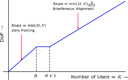
Figure 1: Degrees of freedom for the K user MIMO interference channel [12]

Consider the $K$ user MIMO Gaussian interference channel with $M$ antennas at each transmitter and $N$ antennas at each receiver. The degrees of freedom of this channel are characterized in [12] when the ratio $\frac{\max(M,N)}{\min(M,N)}=R$ is equal to an integer. The main results of [12] are summarized in Fig. 1. As we can see, there are three distinct regimes. For the first regime, i.e., $K\leq R$, there is no competition among the users for degrees of freedom. Each user can access $\min(M,N)$ degree of freedom (the maximum possible) by zero forcing all the interference, regardless of the strength of the interference. The degrees of freedom, as well as the GDOF and the $\mathcal{O}(1)$ capacity characterization in this case are trivial (excluding some degenerate cases). For $K>R$, [12] shows that the degrees of freedom per user cannot be more than $\min(M,N)\frac{R}{R+1}$. For $K>R+1$, the interference alignment problem becomes challenging and the exact degrees of freedom are unknown ([12] provides a tight inner bound only for time-varying/frequency-selective channels) in general, making it difficult to go beyond degrees of freedom. However, if $K=R+1$, the MIMO interference channel has exactly $\min(M,N)\frac{R}{R+1}$ degrees of freedom per user (excluding degenerate cases) and achievability follows by simple zero forcing and time sharing. While the degrees of freedom problem is simple, the competition among the users for the channel degrees of freedom means that the GDOF problem is interesting and depends on the relative strength of the desired and interfering signals. This is the case we study in this paper. Note that for $R=1$ and $M=N=1$, our channel model reduces to the classical two user interference channel and the results, e.g. the W curve, of [1] should be recovered in that case.

I-B Overview of Results

We study the $N+1$ user SIMO Gaussian interference channel with $N$ antennas at each receiver. In order to obtain a compact characterization, we focus on the symmetric case where all direct links have the same signal-to-noise ratio (SNR) and undesired links have the same interference-to-noise ratio (INR). However, no symmetry is assumed for the directions of the channel vectors. Inspired by the connection between the deterministic approach and the GDOF of its Gaussian counterpart, which leads to the constant bits characterization in the two user case, we also would like to first investigate the problem through the corresponding deterministic channel. However, the deterministic channel model proposed in [13] cannot be applied to multiple antennas cases[14]. Instead, we generalize the El Gamal and Costa model [2] to interference channels with multiple antennas. The key assumption of the El Gamal and Costa model for the two user interference channel is the invertibility, i.e., at each receiver, given the desired signal, the interference from the other transmitter can be uniquely determined. This assumption makes this model tractable and also emulates the two user Gaussian interference channel. How to generalize this model to emulate the SIMO Gaussian interference channels? Again the invertibility is essential which also captures the essential feature of this class of SIMO Gaussian interference channels. Consider the 3 user SIMO interference channel with 2 antennas at each receiver. Given the desired signal (in the absence of noise), each receiver can determine the individual interference from each of the interfering transmitters. This is because the number of antennas at each receiver is equal to the number of transmit antennas at all interferers combined. Therefore after the desired signal has been removed, each interference signal is individually isolated by a simple channel matrix inversion operation at each receiver. Thus, we model the SIMO interference channel in the deterministic framework of El Gamal and Costa, by the assumption that, given the signal from the desired transmitter, each receiver is able to recover each of the interfering signals from its received signal. We characterize the capacity region of this deterministic channel. The optimal achievable scheme for this $N+1$ user symmetric deterministic interference channel turns out to be a natural extension of the Han Kobayashi scheme previously shown to be optimal for the 2 user ($N=1$) case. The capacity region for the deterministic channel also reveals interesting new forms of rate bounds that are not trivial extensions of the 2 user case.

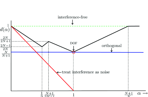
Figure 2: GDOF of the $N+1$ user SIMO Gaussian interference channel with $N$ antennas at each receiver

Based on the insights provided by the deterministic channel, we characterize the generalized degrees of freedom of the $N+1$ user SIMO symmetric Gaussian interference channels with $N$ antennas at each receiver. The GDOF curve is shown in Fig. 2. Note that for $N=1$, the 2 user GDOF of [1] is obtained. Similar to the 2 user Gaussian interference channel with single antenna nodes, there are five distinct regimes. The key elements of the achievability and converse for the GDOF characterization are summarized as follows. In each case, we highlight one major similarity to the 2 user case and one major difference.

1. Achievability:

   • Similarity: The idea of setting the private message power so that it is received at the noise floor of the undesired receivers carries over from the 2 user interference channel.

   • Difference: Unlike the 2 user case, the noisy interference regime disappears from the GDOF picture. Intuitively, this may be understood as follows. The limiting factor for this regime ($\alpha<1/2$) in the 2 user case is the “noise” from the desired users’ private message, which reduces the pre-log factor of the common message rates to zero (The private messages of the remaining users do not matter because they are received at the level of the noise floor). However, in the SIMO case, the noise from the desired users’ private message can be nulled by losing one dimension, while still leaving $N-1$ dimensions to decode the common messages from the remaining $N$ users with a non-zero pre-log factor.

2. Converse:

   • Similarity: The outer bound that is tight for the second “V” of the W curve comes from a “many-to-one” interference channel outer bound. This is the counterpart to the “Z” interference channel sum capacity outer bound used for the corresponding regime in the 2 user case.

   • Difference: The outer bound that is tight for the first “V” of the W curve (the weak interference regime) is a new outer bound which, unlike the two user case, is not in the form of a direct sum-rate bound. For example, with 3 users the outer bound comes from rate bounds that take the form $R_{1}+2R_{2}+R_{3}$. However, as in the 2 user case, the outer bound emerges from studying the El Gamal and Costa deterministic channel model.

The GDOF characterization leads directly to the capacity approximation within $\mathcal{O}(1)$, i.e., the gap to the exact capacity is a constant which is independent of SNR and INR. Instead, the gap depends on other channel parameters, e.g., the angles between channel vectors. To further investigate how angles among channel vectors affect the gap, we study the 3 user completely symmetric Gaussian interference channel with 2 antennas at each receiver. By completely symmetric, we mean that not only all SNRs, INRs are equal, respectively, but also the relative orientations of the desired signal and interference vectors are identical at each receiver. It turns out that the gap only depends on the angle between two interfering vectors (it does not depend on the angle between the desired channel vector and the interfering channel vector). When the angle is large, the gap is small, but if the angle is small, the gap is large. In fact, this angle indicates the possibility of interference alignment. The role of the angles between channel vectors is also highlighted by Wang and Tse in [14] for a three-to-one Gaussian interference channel where only one receiver equipped with 2 antennas sees interference. They show that Han-Kobayashi-type scheme with Gaussian codebook can achieve the capacity region within a number of bits, which depends on the angle between two interfering channel vectors. The gap becomes unbounded when the angle becomes small. Wang and Tse [14] provide a partial interference alignment scheme to get a better performance where the transmit signal is a superposition of Gaussian codewords and lattice codewords. After decoding the Gaussian codewords, the signal is projected onto one direction such that interference alignment can be done using lattice code as in [7]. However, since only one receiver sees interference, the many-to-one setting is significantly different from the fully connected interference channel considered in this work.

We also derive an outer bound on the capacity region of the 3 user SIMO Gaussian interference channel (not necessarily symmetric) with 2 antennas at each receiver. This outer bound directly leads to the capacity region of the strong interference regime of this channel, where each receiver can decode all messages.

II deterministic channel model

II-A El Gamal and Costa Deterministic Channel Model and Connection to the Gaussian Channel

The 2 user deterministic interference channel studied in [2] is shown in Fig. 3. The interference $V_{1},V_{2}$ and channel outputs $Y_{1},Y_{2}$ are deterministic functions of inputs $X_{1},X_{2}$, respectively:

$$V_{1} = g_{1}(X_{1})$$

$$V_{2} = g_{2}(X_{2})$$

$$Y_{1} = f_{1}(X_{1},V_{2})$$

$$Y_{2} = f_{1}(X_{2},V_{1})$$

where $g_{i},f_{i}~{}\forall i=1,2$ are deterministic functions. In addition, $f_{i}$ satisfies conditions

$$H(Y_{1}|X_{1})=H(V_{2})$$ (1)

$$H(Y_{2}|X_{2})=H(V_{1})$$ (2)

for all product distributions on $X_{1}X_{2}$. In other words, given $X_{i}$, function $f_{i}$ is invertible. The capacity region of this class of interference channels is found in [2]. The achievable scheme is the Han-Kobayashi scheme which assigns the common information to interfering signal which is visible to the other link, i.e., $V_{1}$ and $V_{2}$. The connection of this deterministic channel to the two user Gaussian interference channel is discussed in [1]. On the achievability side, it is argued that the portion of the received interfering signal above the noise level, i.e., the interfering signal which is visible to the other link, should be the common information [1]. On the converse side, the outer bounds for the deterministic channel give some hints of what genie information should be given to receivers for the Gaussian case. We further illustrate this point through an example. For the 2 user deterministic interference channel, the sum capacity is shown [2] to be bounded by

$$R_{1}+R_{2}\leq H(Y_{1}|V_{1})+H(Y_{2}|V_{2}).$$ (3)

For the 2 user Gaussian interference channel, a new outer bound derived by Etkin, Tse and Wang [1], which we refer to as the ETW bound, is

$$R_{1}+R_{2}\leq h(y_{1}|s_{1})+h(y_{2}|s_{2})-h(z_{1})-h(z_{2})$$ (4)

where $s_{1}$ and $s_{2}$ are interfering signals from Transmitter 1 and 2, respectively, i.e.,

$$s_{1} = h_{21}x_{1}+z_{2}$$ (5)

$$s_{2} = h_{12}x_{2}+z_{1}$$ (6)

Comparing (3) with (4), we can see that $s_{1}$ and $s_{2}$ for the Gaussian channel are counterparts to $V_{1}$ and $V_{2}$ for the deterministic case. The outer bounds for the deterministic channel and the Gaussian channel are very similar, except that there is no noise terms in the deterministic case. Therefore, the outer bound for the deterministic channel gives some hints of what side information should be given to receivers in the Gaussian case. For example, in order to have $h(y_{1}|s_{1})$ and $h(y_{2}|s_{2})$, we may give $s_{1}$ to Receiver 1 and $s_{2}$ to Receiver 2, which leads to the ETW bound.

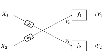
Figure 3: Two user deterministic interference channel [2]

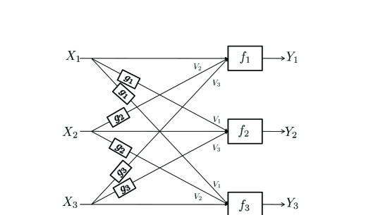
Figure 4: 3 user deterministic interference channel

II-B Deterministic Channel for SIMO Interference Channel

Inspired by the connection of the 2 user deterministic interference channel to the Gaussian case, we would like to study the corresponding deterministic channel of the 3 user SIMO Gaussian interference channel with 2 antennas at each receiver. While we are studying only the 3 user case, the insights from this allow us to tackle the $N+1$ user, $1\times N$ SIMO Gaussian interference channel. Note that the key assumption of the El Gamal and Costa model for the two user interference channel is the invertibility. We model the 3 user $1\times 2$ SIMO interference channel in the deterministic framework of El Gamal and Costa, by the assumption that, given the signal from the desired transmitter, each receiver is able to recover each of the interfering signals from its received signal. This captures the corresponding essential feature of the SIMO Gaussian interference channel. Each receiver has 2 antennas which is equal to the total number of transmit antennas of all interferers. After the desired signal has been removed, each interference signal can be individually isolated by a simple channel matrix inversion operation at each receiver. The deterministic interference channel is shown in Fig. 4. Note that there is some avoidable loss of generality in assuming that the same $V_{1},V_{2},V_{3}$ appear at more than one receiver. This assumption is used primarily to obtain a compact description of the capacity region, which is already cumbersome as we will see later. Also, it is consistent with our ultimate objective of studying the symmetric SIMO Gaussian interference channel.

The interference $V_{1},V_{2},V_{3}$ and channel outputs $Y_{1},Y_{2},Y_{3}$ are deterministic functions of inputs $X_{1},X_{2},X_{3}$, respectively:

$$V_{1} = g_{1}(X_{1})$$

$$V_{2} = g_{2}(X_{2})$$

$$V_{3} = g_{3}(X_{3})$$

$$Y_{1} = f_{1}(X_{1},V_{2},V_{3})$$

$$Y_{2} = f_{1}(X_{2},V_{1},V_{3})$$

$$Y_{3} = f_{1}(X_{3},V_{1},V_{2})$$

where $g_{i},f_{i}~{}\forall i=1,2,3$ are deterministic functions. In addition, $f_{i}$ satisfies conditions

$$H(Y_{1}|X_{1})=H(V_{2}V_{3})=H(V_{2})+H(V_{3})$$ (7)

$$H(Y_{2}|X_{2})=H(V_{1}V_{3})=H(V_{1})+H(V_{3})$$ (8)

$$H(Y_{3}|X_{3})=H(V_{1}V_{2})=H(V_{1})+H(V_{2})$$ (9)

for all product distributions on $X_{1}X_{2}X_{3}$. In other words, given $X_{i}$, function $f_{i}$ is invertible.

Transmitter $i$ has a message $W_{i}\in\{1,\cdots,2^{nR_{i}}\}$ for receiver $i$. A rate tuple $(R_{1},R_{2},R_{3})$ is achievable if $\forall\epsilon>0$ there exists a block length $n$ and encoder $e_{i}$: $\{1,\cdots,2^{nR_{i}}\}~{}\rightarrow~{}\mathcal{X}_{i}^{n}$ and decoder $d_{i}$: $\mathcal{Y}_{i}^{n}~{}\rightarrow~{}\{1,\cdots,2^{nR_{i}}\}$ such that

$$\frac{1}{2^{n(R_{1}+R_{2}+R_{3})}}\sum_{(w_{1},w_{2},w_{3})}\text{Pr}\{(d_{1}(Y_{1}^{n}),d_{2}(Y_{2}^{n}),d_{3}(Y_{3}^{n}))\neq(w_{1},w_{2},w_{3})|W_{1}=w_{1},W_{2}=w_{2},W_{3}=w_{3}\}<\epsilon$$

The capacity region of this channel is the closure of all achievable rate tuples ($R_{1},R_{2},R_{3}$).

III capacity region of the deterministic channel

Define a rate region $\mathcal{R}(1,2,3)$ specified by following inequalities:

$$R_{1} \leq H(Y_{1}|V_{2}V_{3})$$ (10)

$$R_{1}+R_{2} \leq H(Y_{1}|V_{1}V_{2}V_{3})+H(Y_{2}|V_{3})$$ (11)

$$R_{1}+R_{2} \leq H(Y_{1}|V_{1}V_{3})+H(Y_{2}|V_{2}V_{3})$$ (12)

$$2R_{1}+R_{2} \leq H(Y_{1}|V_{3})+H(Y_{1}|V_{1}V_{2}V_{3})+H(Y_{2}|V_{2}V_{3})$$ (13)

$$R_{1}+R_{2}+R_{3} \leq H(Y_{1}|V_{1})+H(Y_{2}|V_{2}V_{3})+H(Y_{3}|V_{1}V_{2}V_{3})$$ (14)

$$R_{1}+R_{2}+R_{3} \leq H(Y_{1}|V_{1}V_{3})+H(Y_{2}|V_{1}V_{2})+H(Y_{3}|V_{2}V_{3})$$ (15)

$$R_{1}+R_{2}+R_{3} \leq H(Y_{1}|V_{1}V_{2}V_{3})+H(Y_{2}|V_{1})+H(Y_{3}|V_{2}V_{3})$$ (16)

$$R_{1}+R_{2}+R_{3} \leq H(Y_{1}|V_{1}V_{2}V_{3})+H(Y_{2}|V_{1}V_{2}V_{3})+H(Y_{3})$$ (17)

$$2R_{1}+R_{2}+R_{3} \leq H(Y_{1})+H(Y_{1}|V_{1}V_{2}V_{3})+H(Y_{2}|V_{2}V_{3})+H(Y_{3}|V_{1}V_{2}V_{3})$$ (18)

$$2R_{1}+R_{2}+R_{3} \leq H(Y_{1}|V_{1})+H(Y_{1}|V_{1}V_{2}V_{3})+H(Y_{2}|V_{2}V_{3})+H(Y_{3}|V_{2}V_{3})$$ (19)

$$2R_{1}+R_{2}+R_{3} \leq H(Y_{1}|V_{1}V_{3})+H(Y_{1}|V_{2})+H(Y_{2}|V_{1}V_{2}V_{3})+H(Y_{3}|V_{2}V_{3})$$ (20)

$$2R_{1}+R_{2}+R_{3} \leq H(Y_{1}|V_{1}V_{2}V_{3})+H(Y_{1}|V_{3})+H(Y_{2}|V_{1}V_{2})+H(Y_{3}|V_{2}V_{3})$$ (21)

$$2R_{1}+R_{2}+R_{3} \leq H(Y_{1}|V_{1}V_{2}V_{3})+H(Y_{1}|V_{3})+H(Y_{2}|V_{2})+H(Y_{3}|V_{1}V_{2}V_{3})$$ (22)

$$2R_{1}+R_{2}+R_{3} \leq H(Y_{1}|V_{1}V_{2}V_{3})+H(Y_{1}|V_{1}V_{2})+H(Y_{2}|V_{2}V_{3})+H(Y_{3}|V_{3})$$ (23)

$$2R_{1}+R_{2}+R_{3} \leq 2H(Y_{1}|V_{1}V_{2}V_{3})+H(Y_{2})+H(Y_{3}|V_{2}V_{3})$$ (24)

$$2R_{1}+R_{2}+R_{3} \leq 2H(Y_{1}|V_{1}V_{2}V_{3})+H(Y_{2}|V_{2})+H(Y_{3}|V_{3})$$ (25)

$$3R_{1}+R_{2}+R_{3} \leq 2H(Y_{1}|V_{1}V_{2}V_{3})+H(Y_{1})+H(Y_{2}|V_{2}V_{3})+H(Y_{3}|V_{2}V_{3})$$ (26)

$$3R_{1}+R_{2}+R_{3} \leq 2H(Y_{1}|V_{1}V_{2}V_{3})+H(Y_{1}|V_{2})+H(Y_{2}|V_{2}V_{3})+H(Y_{3}|V_{3})$$ (27)

$$2R_{1}+2R_{2}+R_{3} \leq H(Y_{1})+H(Y_{1}|V_{1}V_{3})+2H(Y_{2}|V_{1}V_{2}V_{3})+H(Y_{3}|V_{2}V_{3})$$ (28)

$$2R_{1}+2R_{2}+R_{3} \leq H(Y_{1})+H(Y_{1}|V_{1}V_{2}V_{3})+H(Y_{2}|V_{1}V_{2}V_{3})+H(Y_{2}|V_{2}V_{3})+H(Y_{3}|V_{1}V_{3})$$ (29)

$$2R_{1}+2R_{2}+R_{3} \leq H(Y_{1})+H(Y_{1}|V_{1}V_{2}V_{3})+2H(Y_{2}|V_{1}V_{2}V_{3})+H(Y_{3}|V_{3})$$ (30)

$$2R_{1}+2R_{2}+R_{3} \leq H(Y_{1}|V_{1})+H(Y_{1}|V_{1}V_{2}V_{3})+H(Y_{2}|V_{1}V_{2}V_{3})+H(Y_{2}|V_{2}V_{3})+H(Y_{3}|V_{3})$$ (31)

$$2R_{1}+2R_{2}+R_{3} \leq 2H(Y_{1}|V_{1}V_{3})+H(Y_{2}|V_{1}V_{2}V_{3})+H(Y_{2}|V_{2})+H(Y_{3}|V_{2}V_{3})$$ (32)

$$3R_{1}+2R_{2}+R_{3} \leq 2H(Y_{1}|V_{1}V_{2}V_{3})+H(Y_{1})+H(Y_{2}|V_{1}V_{2}V_{3})+H(Y_{2}|V_{2}V_{3})+H(Y_{3}|V_{3})$$ (33)

$$3R_{1}+2R_{2}+R_{3} \leq 2H(Y_{1}|V_{1}V_{2}V_{3})+H(Y_{1})+2H(Y_{2}|V_{2}V_{3})+H(Y_{3}|V_{1}V_{3})$$ (34)

$$3R_{1}+2R_{2}+R_{3} \leq 2H(Y_{1}|V_{1}V_{2}V_{3})+H(Y_{1}|V_{1})+2H(Y_{2}|V_{2}V_{3})+H(Y_{3}|V_{3})$$ (35)

$$3R_{1}+2R_{2}+R_{3} \leq 3H(Y_{1}|V_{1}V_{2}V_{3})+H(Y_{2}|V_{2}V_{3})+H(Y_{2})+H(Y_{3}|V_{3})$$ (36)

$$4R_{1}+2R_{2}+R_{3} \leq 3H(Y_{1}|V_{1}V_{2}V_{3})+H(Y_{1})+2H(Y_{2}|V_{2}V_{3})+H(Y_{3}|V_{3})$$ (37)

Theorem 1

The capacity region of the deterministic channel is the closure of the convex hull of the set of all rate tuples ($R_{1},R_{2},R_{3}$) satisfying the conditions specified by

$$\mathcal{R}(1,2,3)\cup\mathcal{R}(1,3,2)\cup\mathcal{R}(2,1,3)\cup\mathcal{R}(2,3,1)\cup\mathcal{R}(3,1,2)\cup\mathcal{R}(3,2,1)$$

over all product distributions $p_{1}(x_{1})p_{2}(x_{2})p_{3}(x_{3})$.

III-A Achievability

1) Codebook generation: Transmitter $i$, $\forall i=1,2,3$ generates $2^{nR_{ic}}$ independent codewords of length $n$, $V_{i}^{n}(j_{i}),j_{i}\in\{1,2,\cdots,2^{nR_{ic}}\}$, according to $\prod_{k=1}^{n}p_{V_{i}}(v_{ik})$. For each codeword $V_{i}^{n}(j_{i})$, generate $2^{nR_{ip}}$ independent codewords $X^{n}_{i}(j_{i},l_{i})$ according to $\prod_{k=1}^{n}p_{X_{i}|V_{i}}(x_{ik}|v_{ik})$.

2) Encoding: Transmitter $i$ sends codeword $X_{i}^{n}(j_{i},l_{i})$ corresponding to the message indexed by $(j_{i},l_{i})$.

3) Decoding: Receiver $1$ looks for a unique $(\hat{j}_{1},\hat{l}_{1})$ and a pair $(\hat{j}_{2},\hat{j}_{3})$ such that

$$\big{(}X_{1}^{n}(\hat{j}_{1},\hat{l}_{1}),V_{1}^{n}(\hat{j}_{1}),V_{2}^{n}(\hat{j}_{2}),V_{3}^{n}(\hat{j}_{3}),Y_{1}^{n}\big{)}\in A_{n}^{\epsilon}(X_{1},V_{1},V_{2},V_{3},Y_{1}).$$

Similar decoding is done at Receiver 2 and 3.

4) Error Analysis: The detailed analysis is provided in the Appendix. The probability of error at Receiver 1 can be made arbitrarily small as $n\rightarrow\infty$ if the following conditions are satisfied:

$$R_{1p}+R_{1c}+R_{2c}+R_{3c} \leq H(Y_{1})$$ (38)

$$R_{1c}+R_{1p}+R_{2c} \leq H(Y_{1}|V_{3})$$ (39)

$$R_{1c}+R_{1p}+R_{3c} \leq H(Y_{1}|V_{2})$$ (40)

$$R_{1p}+R_{2c}+R_{3c} \leq H(Y_{1}|V_{1})$$ (41)

$$R_{1p}+R_{2c} \leq H(Y_{1}|V_{1}V_{3})$$ (42)

$$R_{1p}+R_{3c} \leq H(Y_{1}|V_{1}V_{2})$$ (43)

$$R_{1c}+R_{1p} \leq H(Y_{1}|V_{2}V_{3})$$ (44)

$$R_{1p} \leq H(Y_{1}|V_{1}V_{2}V_{3})$$ (45)

$$R_{ip},R_{ic} \geq 0~{}\forall i=1,2,3$$ (46)

By swapping indices 1 and 2 everywhere in the $\eqref{condition1}-\eqref{condition8}$, we have the conditions for Receiver 2. Similarly, the conditions for Receiver 3 are obtained by swapping indices 1 and 3 everywhere in $\eqref{condition1}-\eqref{condition8}$. All these conditions specify the achievable rate region for rate vector $(R_{1p},R_{2p},R_{3p},R_{1c},R_{2c},R_{3c})$. Using Fourier-Motzkin elimination with $R_{i}=R_{ic}+R_{ip}$, we have the achievable region as in Theorem 1.

III-B Converse

The proof for the converse uses the following inequality also used in [2]:

$$H(X)-H(Y)\leq H(X|Y)$$ (47)

This is because

$$H(X|Y)+H(Y)=H(X,Y)\geq H(X)$$ (48)

Here we only provide the proof for $4R_{1}+2R_{2}+R_{3}\leq 3H(Y_{1}|V_{1}V_{2}V_{3})+H(Y_{1})+2H(Y_{2}|V_{2}V_{3})+H(Y_{3}|V_{3})$. The proof for all other inequalities can be constructed in the same manner. From Fano’s inequality, we have

$$n(4R_{1}+2R_{2}+R_{3}-7\epsilon_{n})$$

$$\leq 4I(X_{1}^{n};Y_{1}^{n})+2I(X_{2}^{n};Y_{2}^{n})+I(X_{3}^{n};Y_{3}^{n})$$

$$\leq 4H(Y_{1}^{n})-4H(Y_{1}^{n}|X_{1}^{n})+2H(Y_{2}^{n})-2H(Y_{2}^{n}|X^{n}_{2})+H(Y_{3}^{n})-H(Y_{3}^{n}|X^{n}_{3})$$

$$= 4H(Y_{1}^{n})-4H(V_{2}^{n}V_{3}^{n})+2H(Y_{2}^{n})-2H(V_{1}^{n}V_{3}^{n})+H(Y_{3}^{n})-H(V_{1}^{n}V_{2}^{n})$$

$$= 4H(Y_{1}^{n})+2H(Y_{2}^{n})+H(Y_{3}^{n})-3H(V_{1}^{n})-5H(V_{2}^{n})-6H(V_{3}^{n})$$

$$= 3H(Y_{1}^{n})-3H(V_{1}^{n}V_{2}^{n}V_{3}^{n})+H(Y_{1}^{n})+2H(Y_{2}^{n})-2H(V_{2}^{n}V_{3}^{n})+H(Y_{3}^{n})-H(V_{3}^{n})$$

$$\leq 3H(Y_{1}^{n}|V_{1}^{n}V_{2}^{n}V_{3}^{n})+H(Y_{1}^{n})+2H(Y_{2}^{n}|V_{2}^{n}V_{3}^{n})+H(Y_{3}^{n}|V_{3}^{n})$$

$$\leq \sum_{i=1}^{n}(3H(Y_{1i}|V_{1i}V_{2i}V_{3i})+H(Y_{1i})+2H(Y_{2i}|V_{2i}V_{3i})+H(Y_{3i}|V_{3i}))$$

In the derivation above we use assumptions (7), (8), (9) and independence among $V_{1}$, $V_{2}$ and $V_{3}$.

Before we move on to the Gaussian interference channel, we summarize the insights gained from this deterministic channel. On the achievability side, since the Han-Kobayashi scheme which assigns the common information to interfering signal which is visible to each receiver achieves the capacity, we expect that the simple Han-Kobayashi scheme with the private message’s power set to be received at the noise level used in [1] should be good for the SIMO Gaussian interference channel. On the converse side, the outer bounds for the deterministic channel can help us to derive outer bounds for the Gaussian case. Here we highlight two outer bounds which will be used later.

$$R_{1}+R_{2}+R_{3}\leq H(Y_{1}|V_{1}V_{2}V_{3})+H(Y_{2}|V_{1}V_{2}V_{3})+H(Y_{3})$$ (49)

$$R_{1}+2R_{2}+R_{3}\leq H(Y_{1}|V_{1})+2H(Y_{2}|V_{1}V_{2}V_{3})+H(Y_{3}|V_{3})$$ (50)

As we can see, the first one is a many-to-one interference channel outer bound (the counterpart to the Z channel bound in the 2 user case). The second outer bound highlighted above is the basis for the new outer bound that we derive for the Gaussian case, which is tight in the weak interference regime. Note that the corresponding outer bound for the 2 user case is a direct sum rate bound $R_{1}+R_{2}\leq H(Y_{1}|V_{1})+H(Y_{2}|V_{2})$ which leads to the ETW bound.

IV Preliminaries for Symmetric SIMO Gaussian interference channels

IV-A Channel Model

Consider the symmetric $K$ user SIMO Gaussian interference channel, where all direct links have the same signal-to-noise ratio (SNR), and all cross links have the same interference-to-noise ratio (INR). Each transmitter has a single antenna and each receiver has $N$ antennas. The channel’s input-output relationship is described as

$$\mathbf{Y}_{j}=\sqrt{\text{SNR}}\mathbf{H}_{jj}x_{j}+\sqrt{\text{INR}}\sum_{i=1,i\neq j}^{K}\mathbf{H}_{ji}x_{i}+\mathbf{Z}_{j}~{}~{}\forall j=1,\ldots,K$$ (51)

where $\mathbf{Y}_{j}$ is the $N\times 1$ received signal vector at receiver $j$, $\mathbf{H}_{ji}$ is the $N\times 1$ channel vector from transmitter $i$ to receiver $j$, $x_{i}$ is the input signal which satisfies the average power constraint $\mathbf{E}[|x_{i}|^{2}]\leq 1$ and $\mathbf{Z}_{j}$ is the additive circularly symmetric complex Gaussian noise vector with zero mean and identity covariance matrix, i.e., $\mathbf{Z}_{j}\sim\mathcal{CN}(\mathbf{0},\mathbf{I})$. We assume the norm of channel vectors is equal to unity, i.e., $\|\mathbf{H}_{ji}\|=1,\forall i,j=1,2,\cdots,K$. In order to avoid degenerate channel conditions, we assume that the channel coefficients are drawn from a continuous distribution, so that the channel vectors are in general position. For example, if all channel vectors are collinear at each receiver, it is essentially a single input and single output (SISO) channel.

The probability of error, achievable rates $R_{1},\cdots,R_{K}$ and capacity region $\mathcal{C}$ are defined in the standard Shannon sense. Our focus is the symmetric capacity, i.e.,

$$C_{\text{sym}}=\max_{(R,\cdots,R)\in\mathcal{C}}R$$ (52)

IV-B Generalized Degrees of Freedom

As in [1], we define

$$\alpha=\frac{\log{\text{INR}}}{\log{\text{SNR}}}\Rightarrow\text{INR}=\text{SNR}^{\alpha}$$

For simplicity, we denote SNR by $\rho$ and INR by $\rho^{\alpha}$. The generalized degrees of freedom per user are defined as

$$d_{\text{sym}}(\alpha)=\lim_{\rho\rightarrow\infty}\frac{C_{\text{sym}}(\rho,\alpha)}{\log{\rho}}=\frac{1}{K}\lim_{\rho\rightarrow\infty}\frac{C_{\Sigma}(\rho,\alpha)}{\log{\rho}}$$

where $C_{\text{sym}}$ is the symmetric capacity and $C_{\Sigma}$ is the sum capacity.

IV-C $\mathcal{O}(1)$ Approximation

The $\mathcal{O}(1)$ approximation means that the approximation error is bounded as the SNR, INR go to infinity. We will use two $\mathcal{O}(1)$ approximations introduced in [15]. We restate the two approximations from [15] to accommodate to the notations in this paper. The proof can be found in [15] and is omitted here. The first one is the multiple access approximation:

Lemma 1

Suppose $\mathbf{H}_{1}$ is an $N\times r_{1}$ matrix where $r_{1}$ is the rank of $\mathbf{H}_{1}$. $\mathbf{H}_{2}$ is an $N\times r_{2}$ matrix where $r_{2}$ is the rank of $\mathbf{H}_{2}$. For $r_{1}+r_{2}\geq N$ and $\alpha\geq\beta$, almost surely

$$\log|\mathbf{I}+\rho^{\alpha}\mathbf{H}_{1}\mathbf{H}_{1}^{\dagger}+\rho^{\beta}\mathbf{H}_{2}\mathbf{H}_{2}^{\dagger}|=r_{1}\alpha\log\rho+(N-r_{1})\beta\log\rho+\mathcal{O}(1)$$ (53)

The second one is the interference limited approximation:

Lemma 2

For matrices $\mathbf{H}_{1}$ and $\mathbf{H}_{2}$ that satisfy the same conditions in Lemma 1, almost surely

$$\log|\mathbf{I}+(\mathbf{I}+\rho^{\beta}\mathbf{H}_{2}\mathbf{H}_{2}^{\dagger})^{-1}\rho^{\alpha}\mathbf{H}_{1}\mathbf{H}_{1}^{\dagger}|=r_{1}\alpha\log\rho+(N-r_{1}-r_{2})\beta\log\rho+\mathcal{O}(1)$$ (54)

Note that Lemma 2 follows directly from Lemma 1, because

$$\log|\mathbf{I}+(\mathbf{I}+\rho^{\beta}\mathbf{H}_{2}\mathbf{H}_{2}^{\dagger})^{-1}\rho^{\alpha}\mathbf{H}_{1}\mathbf{H}_{1}^{\dagger}|$$

$$= \log|\mathbf{I}+\rho^{\alpha}\mathbf{H}_{1}\mathbf{H}_{1}^{\dagger}+\rho^{\beta}\mathbf{H}_{2}\mathbf{H}_{2}^{\dagger}|-\log|\mathbf{I}+\rho^{\beta}\mathbf{H}_{2}\mathbf{H}_{2}^{\dagger}|$$

$$= r_{1}\alpha\log\rho+(N-r_{1})\beta\log\rho-r_{2}\beta\log\rho+\mathcal{O}(1)$$

$$= r_{1}\alpha\log\rho+(N-r_{1}-r_{2})\beta\log\rho+\mathcal{O}(1)$$

V Generalized Degrees of Freedom of symmetric SIMO Gaussian Interference channels

In this section, we focus on the SIMO Gaussian interference channel when number of users, $K=N+1$ and each receiver has $N$ antennas. The result is presented in the following theorem.

Theorem 2

The generalized degrees of freedom of the $N+1$ user symmetric SIMO Gaussian interference channel with $N$ antennas at each receiver are

$$d_{\text{sym}}(\alpha)=\left\{\begin{array}[]{ccc}1-\frac{\alpha}{N}&{}\hfil&0<\alpha\leq\frac{1}{2}\\ \frac{N-1}{N}+\frac{\alpha}{N}&{}\hfil&\frac{1}{2}\leq\alpha\leq\frac{N+1}{2N+1}\\ 1-\frac{\alpha}{N+1}&{}\hfil&\frac{N+1}{2N+1}\leq\alpha\leq 1\\ \frac{N}{N+1}\alpha&{}\hfil&1\leq\alpha\leq\frac{N+1}{N}\\ 1&{}\hfil&\alpha\geq\frac{N+1}{N}\end{array}\right.$$

Note that for $N=1$, the 2 user GDOF of [1] is obtained. To prove Theorem 2, we derive inner bounds and outer bounds on the GDOF and show that they match for each range of $\alpha$. For comparison, we also plot the GDOF achieved by two suboptimal schemes in Fig. 2: orthogonal transmission and treating interference as noise. We can also make an interesting observation for the very weak interference regime, i.e., $\alpha\leq\frac{1}{2}$. Unlike the $K$ user symmetric Gaussian interference channel with single antenna nodes where treating interference as noise is optimal in terms of GDOF for the very weak interference regime [11], treating interference as noise is strictly suboptimal for the GDOF of the $N+1$ user SIMO interference channel with $N$ antennas at each receiver.

V-A Inner Bounds on the Generalized Degrees of Freedom

We establish the achievable GDOF for each regime in this section.

V-A1 $\alpha\geq 1$

In this regime, the interference is stronger than the desired signal. The achievable scheme is to let every receiver decode all messages. Then, the achievable rate region is the intersection of $N+1$ MAC capacity regions, one at each receiver. The region is specified by

$$\sum_{k\in\mathcal{S}}R_{jk}\leq\log|\mathbf{I}+\sum_{k\in\mathcal{S}}P_{k}\mathbf{H}_{jk}\mathbf{H}_{jk}^{\dagger}|~{}~{}~{}\forall\mathcal{S}\subseteq\{1,2,\cdots,N+1\}$$ (56)

where $P_{k}=\rho^{\alpha}$ if $k\neq j$ and $P_{j}=\rho$. Based on the rate region, we can calculate the generalized degrees of freedom region. For every $\mathcal{S}\neq\{1,\cdots,N+1\}$,

$$\sum_{k\in\mathcal{S}}d_{jk}(\alpha) \leq \left\{\begin{array}[]{cc}|\mathcal{S}|\alpha&j\notin\mathcal{S}\\ (|\mathcal{S}|-1)\alpha+1&j\in\mathcal{S}\end{array}\right.$$ (59)

$$\Rightarrow d_{\text{sym}}(\alpha) \leq 1$$ (60)

Note that $d_{\text{sym}}(\alpha)$ is the GDOF per user. For $\mathcal{S}=\{1,\cdots,N+1\}$,

$$\sum_{k\in\mathcal{S}}d_{jk}(\alpha)\leq N\alpha\Rightarrow d_{\text{sym}}(\alpha)\leq\frac{N}{N+1}\alpha$$ (61)

From (60), (61), we can see that the achievable symmetric degrees of freedom is $\min\{1,\frac{N}{N+1}\alpha\}$. Therefore,

$$d_{\text{sym}}(\alpha)=\left\{\begin{array}[]{cc}1&\alpha\geq\frac{N+1}{N}\\ \frac{N}{N+1}\alpha&1\leq\alpha\leq\frac{N+1}{N}\end{array}\right.$$

V-A2 $0\leq\alpha\leq 1$

This is the weak interference regime. The transmission scheme is a natural generalization of the simple Han-Kobayashi type scheme used in [1]. Transmitter $j,\forall j=1,\ldots,N+1$ splits its message $W_{j}$ into two sub-messages: a common message $W_{j,c}$ and a private message $W_{j,p}$. The common message will be decoded by all receivers while the private message is only decoded by the desired receiver. The common message $W_{j,c}$ is encoded using a Gaussian codebook with rate $R_{j,c}$ and power $P_{j,c}$. The private message $W_{j,p}$ is encoded using a Gaussian codebook with rate $R_{j,p}$ and power $P_{j,p}$. We set $R_{j,c}=R_{c}$ and $R_{j,p}=R_{p}$. In addition, $P_{j,c}=P_{c}$ and $P_{j,p}=P_{p}$ such that $P_{p}+P_{c}=1$. Moreover, the private power $P_{p}$ is set such that the private message is received at the noise floor at the unintended receiver, i.e. $\rho^{\alpha}P_{p}=1$. If $\rho^{\alpha}<1$, then set $P_{p}=1$. For this case, there is no common message and each receiver decodes its message by treating interference as noise. Finally, the transmitted signal $x_{j}$ is the superposition of the common and private signals. The decoding order is fixed as decoding the common messages first while decoding the private message last. The achievable scheme for $N=2$ is illustrated in Fig. 5.

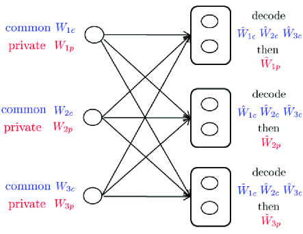
Figure 5: Achievable scheme for 3 user $1\times 2$ SIMO interference channel in the weak interference regime ($0\leq\alpha\leq 1$)

To calculate the achievable rate using this scheme, it is useful to determine the received SNR (INR) of the common messages and private messages at the desired (unintended) receivers. Let $\text{SNR}_{c}$, $\text{SNR}_{p}$, $\text{INR}_{c}$ and $\text{INR}_{p}$ denote the received SNR for common messages and private messages at the desired receiver, and the received INR for common messages and private messages at the unintended receivers, respectively. It can be easily seen that

$$\text{SNR}_{c}=\rho-\rho^{1-\alpha},~{}~{}\text{SNR}_{p}=\rho^{1-\alpha},~{}~{}\text{INR}_{c}=\rho^{\alpha}-1,~{}~{}\text{INR}_{p}=1$$

We first calculate the rate for the private messages. Since the private message is decoded after the common messages are decoded, it is decoded by treating the private messages from unintended transmitters as noise.

$$R_{p} = \min_{j}\{\log|\mathbf{I}+(\mathbf{I}+\sum_{j\neq i}\mathbf{H}_{ji}\mathbf{H}^{{\dagger}}_{ji})^{-1}\rho^{1-\alpha}\mathbf{H}_{jj}\mathbf{H}_{jj}^{{\dagger}}|\}$$ (63)

$$= (1-\alpha)\log\rho+\mathcal{O}(1)$$ (64)

Therefore,

$$d_{p}(\alpha)=1-\alpha$$ (65)

The achievable rate region for the common messages is the intersection of $N+1$ MAC capacity regions, one at each receiver. Due to symmetry, consider the MAC at Receiver 1. Since the common messages are decoded first by treating private messages as noise, the achievable rate region is described by the $N+1$ user MAC constraints, i.e., $\forall\mathcal{S}\subseteq\{1,2,\cdots,N+1\}$

$$\sum_{k\in\mathcal{S}}R_{kc}\leq\log|\mathbf{I}+(\mathbf{I}+\sum_{i\neq 1}\mathbf{H}_{1i}\mathbf{H}^{{\dagger}}_{1i}+\rho^{1-\alpha}\mathbf{H}_{11}\mathbf{H}_{11}^{{\dagger}})^{-1}\sum_{k\in\mathcal{S}}P_{ck}\mathbf{H}_{1k}\mathbf{H}_{1k}^{\dagger}|$$ (66)

where $P_{ck}=\rho^{\alpha}-1$ if $k\neq 1$ and $P_{c1}=\rho-\rho^{1-\alpha}$. Based on the rate region, we can calculate the generalized degrees of freedom region. First, for every $\mathcal{S}\neq\{2,3,\cdots,N+1\}$ or $\{1,2,\cdots,N+1\}$,

$$\log|\mathbf{I}+(\mathbf{I}+\sum_{i\neq 1}\mathbf{H}_{1i}\mathbf{H}^{{\dagger}}_{1i}+\rho^{1-\alpha}\mathbf{H}_{11}\mathbf{H}_{11}^{{\dagger}})^{-1}\sum_{k\in\mathcal{S}}P_{ck}\mathbf{H}_{1k}\mathbf{H}_{1k}^{\dagger}|$$ (67)

$$= \log|\mathbf{I}+\sum_{i\neq 1}\mathbf{H}_{1i}\mathbf{H}^{{\dagger}}_{1i}+\rho^{1-\alpha}\mathbf{H}_{11}\mathbf{H}_{11}^{{\dagger}}+\sum_{k\in\mathcal{S}}P_{ck}\mathbf{H}_{1k}\mathbf{H}_{1k}^{\dagger}|-\log|\mathbf{I}+\sum_{i\neq 1}\mathbf{H}_{1i}\mathbf{H}^{{\dagger}}_{1i}+\rho^{1-\alpha}\mathbf{H}_{11}\mathbf{H}_{11}^{{\dagger}}|$$

If $1\in\mathcal{S}$, then (67) is

$$\log|\mathbf{I}+\sum_{i\neq 1,i\notin\mathcal{S}}\mathbf{H}_{1i}\mathbf{H}^{{\dagger}}_{1i}+\rho\mathbf{H}_{11}\mathbf{H}_{11}^{{\dagger}}+\sum_{k\in\mathcal{S},k\neq 1}\rho^{\alpha}\mathbf{H}_{1k}\mathbf{H}_{1k}^{\dagger}|-\log|\mathbf{I}+\sum_{i\neq 1}\mathbf{H}_{1i}\mathbf{H}^{{\dagger}}_{1i}+\rho^{1-\alpha}\mathbf{H}_{11}\mathbf{H}_{11}^{{\dagger}}|$$ (68)

$$\stackrel{{\scriptstyle(a)}}{{=}} \log|\mathbf{I}+\rho\mathbf{H}_{11}\mathbf{H}_{11}^{{\dagger}}+\sum_{k\in\mathcal{S},k\neq 1}\rho^{\alpha}\mathbf{H}_{1k}\mathbf{H}_{1k}^{\dagger}|-\log|\mathbf{I}+\sum_{i\neq 1}\mathbf{H}_{1i}\mathbf{H}^{{\dagger}}_{1i}+\rho^{1-\alpha}\mathbf{H}_{11}\mathbf{H}_{11}^{{\dagger}}|+\mathcal{O}(1)$$

$$\stackrel{{\scriptstyle(b)}}{{=}} (1+(|\mathcal{S}|-1)\alpha)\log\rho-(1-\alpha)\log\rho+\mathcal{O}(1)$$ (69)

$$= |\mathcal{S}|\alpha\log\rho+\mathcal{O}(1)$$ (70)

where $(a)$ follows from the fact that $\sum_{i\neq 1,i\notin\mathcal{S}}\mathbf{H}_{1i}\mathbf{H}^{{\dagger}}_{1i}$ is constant and $(b)$ follows from Lemma 1. If $1\notin\mathcal{S}$, then (67) is

$$\log|\mathbf{I}+\sum_{i\neq 1,i\notin\mathcal{S}}\mathbf{H}_{1i}\mathbf{H}^{{\dagger}}_{1i}+\rho^{1-\alpha}\mathbf{H}_{11}\mathbf{H}_{11}^{{\dagger}}+\sum_{k\in\mathcal{S}}\rho^{\alpha}\mathbf{H}_{1k}\mathbf{H}_{1k}^{\dagger}|-\log|\mathbf{I}+\sum_{i\neq 1}\mathbf{H}_{1i}\mathbf{H}^{{\dagger}}_{1i}+\rho^{1-\alpha}\mathbf{H}_{11}\mathbf{H}_{11}^{{\dagger}}|$$ (71)

$$= (1-\alpha+|\mathcal{S}|\alpha)\log\rho-(1-\alpha)\log\rho+\mathcal{O}(1)$$

$$= |\mathcal{S}|\alpha\log\rho+\mathcal{O}(1)$$ (72)

Thus,

$$\sum_{k\in\mathcal{S}}d_{kc}(\alpha)\leq|\mathcal{S}|\alpha$$ (73)

$$\Rightarrow d_{c}(\alpha)\leq\alpha$$ (74)

For $\mathcal{S}=\{2,3,\cdots,N+1\}$,

$$R_{2c}+\cdots+R_{(N+1)c}$$ (75)

$$\leq \log|\mathbf{I}+(\mathbf{I}+\sum_{i=2}^{N+1}\mathbf{H}_{1i}\mathbf{H}^{{\dagger}}_{1i}+\rho^{1-\alpha}\mathbf{H}_{11}\mathbf{H}_{11}^{{\dagger}})^{-1}(\rho^{\alpha}-1)\sum_{i=2}^{N+1}\mathbf{H}_{1i}\mathbf{H}^{{\dagger}}_{1i}|$$

$$= \log|\mathbf{I}+\rho^{\alpha}\sum_{i=2}^{N+1}\mathbf{H}_{1i}\mathbf{H}^{{\dagger}}_{1i}+\rho^{1-\alpha}\mathbf{H}_{11}\mathbf{H}_{11}^{{\dagger}}|-\log|\mathbf{I}+\sum_{i=2}^{N+1}\mathbf{H}_{1i}\mathbf{H}^{{\dagger}}_{1i}+\rho^{1-\alpha}\mathbf{H}_{11}\mathbf{H}_{11}^{{\dagger}}|$$ (76)

$$\stackrel{{\scriptstyle(a)}}{{=}} (\max\{\alpha,1-\alpha\}+(N-1)\alpha-(1-\alpha))\log\rho+\mathcal{O}(1)$$ (77)

$$= \max\{(N+1)\alpha-1,(N-1)\alpha\}\log\rho+\mathcal{O}(1)$$ (78)

where (a) follow from Lemma 1. Hence,

$$d_{2c}(\alpha)+\cdots+d_{(N+1)c}(\alpha)\leq\max\{(N+1)\alpha-1,(N-1)\alpha\}$$ (79)

$$\Rightarrow d_{c}(\alpha)\leq\frac{1}{N}\max\{(N+1)\alpha-1,(N-1)\alpha\}$$ (80)

For $\mathcal{S}=\{1,2,\cdots,N+1\}$,

$$R_{1c}+\cdots+R_{(N+1)c}$$ (81)

$$\leq \log|\mathbf{I}+(\mathbf{I}+\sum_{i=2}^{N+1}\mathbf{H}_{1i}\mathbf{H}^{{\dagger}}_{1i}+\rho^{1-\alpha}\mathbf{H}_{11}\mathbf{H}_{11}^{{\dagger}})^{-1}[(\rho-\rho^{1-\alpha})\mathbf{H}_{11}\mathbf{H}_{11}^{{\dagger}}+(\rho^{\alpha}-1)\sum_{i=2}^{N+1}\mathbf{H}_{1i}\mathbf{H}^{{\dagger}}_{1i}]|$$

$$= \log|\mathbf{I}+\rho\mathbf{H}_{11}\mathbf{H}_{11}^{{\dagger}}+\rho^{\alpha}\sum_{i=2}^{N+1}\mathbf{H}_{1i}\mathbf{H}^{{\dagger}}_{1i}|-\log|\mathbf{I}+\sum_{i=2}^{N+1}\mathbf{H}_{1i}\mathbf{H}^{{\dagger}}_{1i}+\rho^{1-\alpha}\mathbf{H}_{11}\mathbf{H}_{11}^{{\dagger}}|$$ (82)

$$= (1+(N-1)\alpha-(1-\alpha))\log\rho+\mathcal{O}(1)$$ (83)

$$= N\alpha\log\rho+\mathcal{O}(1)$$ (84)

Hence,

$$d_{1c}(\alpha)+\cdots+d_{(N+1)c}(\alpha)\leq N\alpha$$ (85)

$$\Rightarrow d_{c}(\alpha)\leq\frac{N}{N+1}\alpha$$ (86)

Due to symmetry, there are similar MAC constraints at each receiver. The achievable rate region is the intersection of the MAC capacity regions of each receiver. Note that only two sum constraints may be active in terms of GDOF depending on $\alpha$. One is the sum rate of all interfering messages given by (80). The other one is the sum rate of all messages given by (86). The maximum achievable symmetric generalized degrees of freedom in this rate region is

$$d_{c}(\alpha)=\min\{\frac{N\alpha}{N+1},\max\{\frac{(N+1)\alpha-1}{N},\frac{(N-1)\alpha}{N}\}\}$$ (87)

From (87), we have

$$d_{c}(\alpha)=\left\{\begin{array}[]{ccc}\frac{(N-1)\alpha}{N}&{}\hfil&0\leq\alpha\leq\frac{1}{2}\\ \frac{(N+1)\alpha-1}{N}&{}\hfil&\frac{1}{2}\leq\alpha\leq\frac{N+1}{2N+1}\\ \frac{N\alpha}{N+1}&{}\hfil&\frac{N+1}{2N+1}\leq\alpha\leq 1\end{array}\right.$$

Therefore, the symmetric generalized degrees of freedom are

$$d_{\text{sym}}(\alpha)=d_{c}(\alpha)+d_{p}(\alpha)=\left\{\begin{array}[]{ccc}1-\frac{\alpha}{N}&{}\hfil&0\leq\alpha\leq\frac{1}{2}\\ \frac{N-1}{N}+\frac{\alpha}{N}&{}\hfil&\frac{1}{2}\leq\alpha\leq\frac{N+1}{2N+1}\\ 1-\frac{\alpha}{N+1}&{}\hfil&\frac{N+1}{2N+1}\leq\alpha\leq 1\end{array}\right.$$

It is interesting to compare the achievable GDOF using this scheme with that achieved by treating all interference as noise. The rate achieved by treating interference as noise is

$$R = \min_{j}\{\log|\mathbf{I}+(\mathbf{I}+\rho^{\alpha}\sum_{j\neq i}\mathbf{H}_{ji}\mathbf{H}^{{\dagger}}_{ji})^{-1}\rho\mathbf{H}_{jj}\mathbf{H}^{{\dagger}}_{jj}|\}$$

$$= (1-\alpha)\log\rho+\mathcal{O}(1)$$

Therefore, the GDOF achieved by treating interference as noise is $d(\alpha)=1-\alpha$, which is strictly less optimal than that achieved using Han-Kobayashi type scheme.

Recall that for the 2 user interference channel with single antenna nodes, when $\alpha\leq\frac{1}{2}$, treating interference as noise is optimal in terms of GDOF. Why is treating interference as noise so suboptimal for the SIMO case? Notice that the private message already achieves $1-\alpha$ degrees of freedom which is the same as that achieved by treating interference as noise. Therefore, whether the Han-Kobayashi scheme is able to achieve more degrees of freedom depends on if the common messages can achieve a non-zero degrees of freedom. Let us first consider the 2 user SISO interference channel. The common messages are decoded first by treating private messages as noise. Due to symmetry, let us consider Receiver 1. Although the private message from Transmitter 2 is received at the noise floor, the private message from Transmitter 1 is received at power $\rho^{1-\alpha}$. This essentially raises the noise floor by $\rho^{1-\alpha}$ at the receiver when decoding the common messages. When $\alpha\leq\frac{1}{2}$, the degrees of freedom of the common message is limited by the degrees of freedom achieved by the common message from the interfering transmitter. The common message from Transmitter 2 is received roughly with power $\rho^{\alpha}$, which is below the noise level, resulting in zero degrees of freedom. This is illustrated in Fig. 6(a).

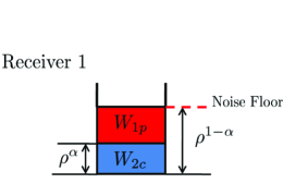
(a) 2 user SISO interference channel

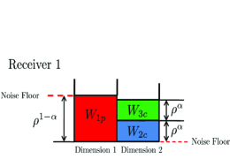
(b) 3 user $1\times 2$ SIMO interference channel

Figure 6: Power of common messages in Receiver 1’s signal space for 2 user SISO interference channel and 3 user $1\times 2$ SIMO case

Now let us consider the $N+1$ user, $1\times N$ SIMO interference channel. For simplicity, consider the case when $N=2$. Again, the private message achieves $1-\alpha$ degrees of freedom. Different from the 2 user SISO case, common messages can achieve positive degrees of freedom. Due to symmetry, let us consider Receiver 1. For the $1\times 2$ SIMO interference channel, the receiver has a 2 dimensional signal space. The desired signal along channel vector $\mathbf{H}_{11}$ occupies one dimension. In this one dimensional subspace, similar to the analysis for the 2 user SISO case, Transmitter 1’s private message is received at power $\rho^{1-\alpha}$ raising the noise level in this dimension; however, in the other dimension, the noise level is not affected. Thus, the common messages from Transmitter 2 and 3 together can achieve $\alpha$ degrees of freedom in that orthogonal dimension. This is illustrated in Fig. 6(b).

V-B Outer bounds for the Generalized Degrees of Freedom

We present three outer bounds which are tight for different regimes.

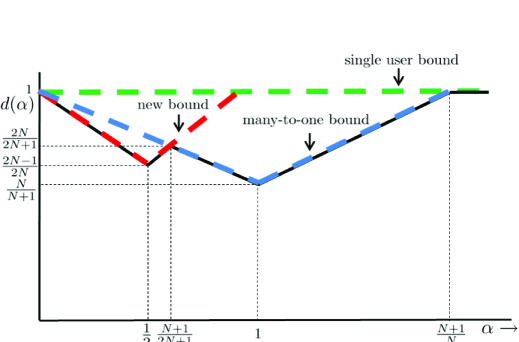
Figure 7: Outer bounds for $N+1$ user $1\times N$ SIMO interference channel

V-B1 Single user bound

For the point to point channel with a single transmit antenna and $N$ receive antennas, the degrees of freedom is 1. The generalized degrees of freedom per user cannot be more than 1 with interference, i.e., $d(\alpha)\leq 1$. As shown in Fig. 7, this bound is tight for very strong interference regime, i.e, $\alpha\geq\frac{N+1}{N}$.

V-B2 Many-to-one outer bound

We first derive an outer bound for the general $K$ user SIMO Gaussian interference channel (not necessarily symmetric) with $N$ antennas at each receiver. The channel is given by

$$\mathbf{Y}_{j}=\sum_{i=1}^{K}\mathbf{H}_{ji}x_{i}+\mathbf{Z}_{j}\quad\forall j=1,\cdots,K$$

where $E[|x_{i}|^{2}]\leq P_{i}$ and $\mathbf{Z}_{j}\sim\mathcal{CN}(\mathbf{0},\mathbf{I})$.

Lemma 3

For the $K$ user SIMO Gaussian interference channel with $N$ antennas at each receiver, the sum capacity is bounded above by

$$R_{\text{sum}} \leq \log|\mathbf{I}+(\mathbf{I}+\sum_{i=2}^{K}P_{i}\mathbf{H}_{1i}\mathbf{H}_{1i}^{\dagger})^{-1}P_{1}\mathbf{H}_{11}\mathbf{H}_{11}^{\dagger}|+\sum_{i=2}^{K}\log(1+P_{i}\|\mathbf{H}_{ii}\|^{2})$$ (90)

$$+\log|\mathbf{I}+\sum_{i=2}^{K}\frac{P_{i}}{1+\|\mathbf{H}_{ii}\|^{2}P_{i}}\mathbf{H}_{1i}\mathbf{H}_{1i}^{\dagger}|$$

Proof:

This outer bound is a natural generalization of the one-sided interference channel outer bound for the two user interference channel with single antenna nodes [1]. More specifically, we will derive an outer bound on the interference channel where only Receiver 1 sees interference. Clearly, this outer bound is also an outer bound for the original interference channel. Suppose the genie provides side information $x_{i}$, $\forall i=1,\ldots,K~{}i\neq j$ to Receiver $j$ $\forall j=2,\ldots,K$. That is, for all receiver but Receiver 1, the genie provides all interference signals to it. So Receiver $j$ $\forall j=2,\ldots,K$ can subtract the interference from their received signals. Then, the genie-aided channel is

$$\mathbf{Y}_{1} = \mathbf{H}_{11}x_{1}+\mathbf{H}_{12}x_{2}+\cdots+\mathbf{H}_{1K}x_{K}+\mathbf{Z}_{1}$$ (91)

$$= \mathbf{H}_{11}x_{1}+\underline{\mathbf{H}}_{12}\underline{\mathbf{X}}_{2}+\mathbf{Z}_{1}$$

$$\mathbf{Y^{\prime}}_{j} = \mathbf{H}_{jj}x_{j}+\mathbf{Z}_{j}~{}\forall j=2,\ldots,K$$ (92)

where $\underline{\mathbf{H}}_{12}=[\mathbf{H}_{12}~{}\cdots~{}\mathbf{H}_{1K}]$. (92) is equivalent to

$$y_{j}=\|\mathbf{H}_{jj}\|x_{j}+z_{j}$$

where $z_{j}\sim\mathcal{CN}(0,1)$. Now let all transmitters but Transmitter 1 cooperate as one transmitter and their corresponding receivers cooperate as one receiver. Then it is equivalent to a two user one-sided interference channel. Since allowing transmitters to cooperate cannot decrease the capacity, the capacity region of this channel is an outer bound of the capacity region of the genie-aided channel. The received signal at Receiver 2 of this two user one-sided interference channel is

$$\underline{\mathbf{Y}}_{2}=\underline{\mathbf{H}}_{2}\underline{\mathbf{X}}_{2}+\underline{\mathbf{Z}}_{2}$$

where $\underline{\mathbf{Y}}_{2}=[y_{2}~{}\cdots~{}y_{K}]^{T}$, $\underline{\mathbf{Z}}_{2}=[z_{2}~{}\cdots~{}z_{K}]^{T}$ and

$$\underline{\mathbf{H}}_{2} = \left[\begin{array}[]{ccc}\|\mathbf{H}_{22}\|&\cdots&0\\ \vdots&\ddots&\vdots\\ 0&\cdots&\|\mathbf{H}_{KK}\|\end{array}\right].$$

Now we can bound the sum rate on this two user one-sided interference channel by providing side information $\mathbf{S}=\underline{\mathbf{H}}_{12}\underline{\mathbf{X}}_{2}+\mathbf{Z}_{1}$ to Receiver 2. Starting from Fano’s inequality, we have

$$nR_{\text{sum}}-n\epsilon_{n}$$ (94)

$$\leq I(x_{1}^{n};\mathbf{Y}_{1}^{n})+I(\underline{\mathbf{X}}_{2}^{n};\underline{\mathbf{Y}}_{2}^{n},\mathbf{S}^{n})$$

$$= h(\mathbf{Y}_{1}^{n})-h(\mathbf{Y}_{1}^{n}|x_{1}^{n})+I(\underline{\mathbf{X}}_{2}^{n};\mathbf{S}^{n})+I(\underline{\mathbf{X}}_{2}^{n};\underline{\mathbf{Y}}_{2}^{n}|\mathbf{S}^{n})$$

$$= h(\mathbf{Y}_{1}^{n})-h(\mathbf{S}^{n})+h(\mathbf{S}^{n})-h(\mathbf{S}^{n}|\underline{\mathbf{X}}_{2}^{n})+I(\underline{\mathbf{X}}_{2}^{n};\underline{\mathbf{Y}}_{2}^{n}|\mathbf{S}^{n})$$

$$= h(\mathbf{Y}_{1}^{n})-h(\mathbf{Z}_{1}^{n})+h(\underline{\mathbf{Y}}_{2}^{n}|\mathbf{S}^{n})-h(\underline{\mathbf{Z}}_{2}^{n}|\mathbf{Z}_{1}^{n})$$

$$\stackrel{{\scriptstyle(a)}}{{\leq}} nh(\mathbf{Y}_{1}^{*})-nh(\mathbf{Z}_{1})+nh(\underline{\mathbf{Y}}_{2}^{*}|\mathbf{S}^{*})-nh(\underline{\mathbf{Z}}_{2}|\mathbf{Z}_{1})$$

$$= nI(x_{1}^{*};\mathbf{Y}_{1}^{*})+nI(\underline{\mathbf{X}}_{2}^{*};\underline{\mathbf{Y}}_{2}^{*},\mathbf{S}^{*})$$ (95)

where * denotes the inputs are i.i.d Gaussian with maximum power, i.e. $x_{i}^{*}\sim\mathcal{CN}(0,P_{i})$ and $\mathbf{Y}_{i}^{*}$ and $\mathbf{S}^{*}$ are the corresponding signals. The fact that $h(\underline{\mathbf{Y}}_{2}^{n}|\mathbf{S}^{n})\leq nh(\underline{\mathbf{Y}}_{2}^{*}|\mathbf{S}^{*})$ in step (a) follows from Lemma 1 in [5].

Now we calculate each term in (95). First,

$$I(x_{1}^{*};\mathbf{Y}_{1}^{*})=\log|\mathbf{I}+(\mathbf{I}+\sum_{i=2}^{K}P_{i}\mathbf{H}_{1i}\mathbf{H}_{1i}^{\dagger})^{-1}P_{1}\mathbf{H}_{11}\mathbf{H}_{11}^{\dagger}|$$ (96)

Since $I(\underline{\mathbf{X}}_{2}^{*};\underline{\mathbf{Y}}_{2}^{*},\mathbf{S}^{*})=I(\underline{\mathbf{X}}_{2}^{*};\underline{\mathbf{Y}}_{2}^{*})+I(\underline{\mathbf{X}}_{2}^{*};\mathbf{S}^{*}|\underline{\mathbf{Y}}_{2}^{*})$ where

$$I(\underline{\mathbf{X}}_{2}^{*};\underline{\mathbf{Y}}_{2}^{*})=\sum_{i=2}^{K}\log(1+P_{i}\|\mathbf{H}_{ii}\|^{2})$$ (97)

and $I(\underline{\mathbf{X}}_{2}^{*};\mathbf{S}^{*}|\underline{\mathbf{Y}}_{2}^{*})=h(\mathbf{S}^{*}|\underline{\mathbf{Y}}_{2}^{*})-h(\mathbf{S}^{*}|\underline{\mathbf{Y}}_{2}^{*},\underline{\mathbf{X}}_{2}^{*})$. Let $\Sigma_{\mathbf{S}^{*}|\underline{\mathbf{Y}}_{2}^{*}}$ be the covariance matrix of $\mathbf{S}^{*}|\underline{\mathbf{Y}}_{2}^{*}$. Then

$$h(\mathbf{S}^{*}|\underline{\mathbf{Y}}_{2}^{*})=\log|\pi e\Sigma_{\mathbf{S}^{*}|\underline{\mathbf{Y}}_{2}^{*}}|$$

where

$$\Sigma_{\mathbf{S}^{*}|\underline{\mathbf{Y}}_{2}^{*}} = E[\mathbf{S}^{*}\mathbf{S}^{*\dagger}]-E[\mathbf{S}^{*}\underline{\mathbf{Y}}_{2}^{*\dagger}]E[\underline{\mathbf{Y}}_{2}^{*}\underline{\mathbf{Y}}_{2}^{*\dagger}]^{-1}E[\underline{\mathbf{Y}}_{2}^{*}\mathbf{S}^{*\dagger}]$$

$$= \mathbf{I}+\mathbf{\underline{H}}_{12}\mathbf{P}_{2}\mathbf{\underline{H}}_{12}^{\dagger}-\mathbf{\underline{H}}_{12}\mathbf{P}_{2}\mathbf{\underline{H}}_{2}^{\dagger}(\mathbf{I}+\mathbf{\underline{H}}_{2}\mathbf{P}_{2}\mathbf{\underline{H}}_{2}^{\dagger})^{-1}\mathbf{\underline{H}}_{2}\mathbf{P}_{2}\mathbf{\underline{H}}_{12}^{\dagger}$$

$$= \mathbf{I}+\mathbf{\underline{H}}_{12}\big{(}\mathbf{P}_{2}-\mathbf{P}_{2}\mathbf{\underline{H}}_{2}^{\dagger}(\mathbf{I}+\mathbf{\underline{H}}_{2}\mathbf{P}_{2}\mathbf{\underline{H}}_{2}^{\dagger})^{-1}\mathbf{\underline{H}}_{2}\mathbf{P}_{2}\big{)}\mathbf{\underline{H}}_{12}^{\dagger}$$

$$\stackrel{{\scriptstyle(a)}}{{=}} \mathbf{I}+\mathbf{\underline{H}}_{12}(\mathbf{P}_{2}^{-1}+\mathbf{\underline{H}}_{2}^{\dagger}\mathbf{\underline{H}}_{2})^{-1}\mathbf{\underline{H}}_{12}^{\dagger}$$

where $(a)$ follows from Woodbury matrix identity [16], which is

$$(\mathbf{A}+\mathbf{B}\mathbf{C}\mathbf{D})^{-1}=\mathbf{A}^{-1}-\mathbf{A}^{-1}\mathbf{B}(\mathbf{C}^{-1}+\mathbf{D}\mathbf{A}^{-1}\mathbf{B})^{-1}\mathbf{D}\mathbf{A}^{-1}$$ (98)

where $\mathbf{A}$, $\mathbf{B}$, $\mathbf{C}$ and $\mathbf{D}$ are $n\times n$, $n\times k$, $k\times k$ and $k\times n$ matrices, respectively. And

$$\mathbf{\underline{H}}_{2}^{\dagger}\mathbf{\underline{H}}_{2}=\left[\begin{array}[]{ccc}\|\mathbf{H}_{22}\|^{2}&\cdots&0\\ \vdots&\ddots&\vdots\\ 0&\cdots&\|\mathbf{H}_{KK}\|^{2}\end{array}\right]\quad\mathbf{P}_{2}=\left[\begin{array}[]{ccc}P_{2}&\cdots&0\\ \vdots&\ddots&\vdots\\ 0&\cdots&P_{K}\end{array}\right]$$

Therefore, we have

$$h(\mathbf{S}^{*}|\underline{\mathbf{Y}}_{2}^{*})=\log|\pi e(\mathbf{I}+\mathbf{\underline{H}}_{12}(\mathbf{P}_{2}^{-1}+\mathbf{\underline{H}}_{2}^{\dagger}\mathbf{\underline{H}}_{2})^{-1}\mathbf{\underline{H}}_{12}^{\dagger})|$$ (100)

and

$$I(\underline{\mathbf{X}}_{2}^{*};\mathbf{S}^{*}|\underline{\mathbf{Y}}_{2}^{*}) = h(\mathbf{S}^{*}|\underline{\mathbf{Y}}_{2}^{*})-h(\mathbf{S}^{*}|\underline{\mathbf{Y}}_{2}^{*},\underline{\mathbf{X}}_{2}^{*})$$

$$= h(\mathbf{S}^{*}|\underline{\mathbf{Y}}_{2}^{*})-h(\mathbf{Z}_{1})$$

$$= \log|\pi e(\mathbf{I}+\mathbf{\underline{H}}_{12}(\mathbf{P}_{2}^{-1}+\mathbf{\underline{H}}_{2}^{\dagger}\mathbf{\underline{H}}_{2})^{-1}\mathbf{\underline{H}}_{12}^{\dagger})|-N\log(\pi e)$$

$$= \log|\mathbf{I}+\mathbf{\underline{H}}_{12}(\mathbf{P}_{2}^{-1}+\mathbf{\underline{H}}_{2}^{\dagger}\mathbf{\underline{H}}_{2})^{-1}\mathbf{\underline{H}}_{12}^{\dagger}|$$ (102)

$$= \log|\mathbf{I}+\sum_{i=2}^{K}\frac{P_{i}}{1+\|\mathbf{H}_{ii}\|^{2}P_{i}}\mathbf{H}_{1i}\mathbf{H}_{1i}^{\dagger}|$$ (103)

Adding (96), (97) and (103), we prove the lemma. ∎

Applying the outer bound to the symmetric case, we have an outer bound for the GDOF which is tight in the regime where $\frac{N+1}{2N+1}\leq\alpha\leq\frac{N+1}{N}$. Before we present the GDOF bound, let us see intuitively why this bound is good for $\frac{N+1}{2N+1}\leq\alpha\leq\frac{N+1}{N}$. Recall that in this regime, at Receiver 1 the MAC constraint that is active for the common messages is $R_{1c}+\cdots+R_{(N+1)c}$. Notice that the received signal $\mathbf{Y}_{1}^{*}$ at Receiver 1 roughly contains common information from Transmitter 1 to $N+1$ and private message from Transmitter 1. Since the power of private messages from Transmitter 2 to $N+1$ is at noise floor at Receiver 1, they do not reveal to Receiver 1. Therefore, we can think that $R_{1}+R_{2c}+\cdots+R_{(N+1)c}\leq h(\mathbf{Y}_{1}^{*})-h(\mathbf{Z}_{1})$. On the other hand, $\underline{\mathbf{Y}}_{2}^{*}|\mathbf{S}^{*}$ roughly contains the private information from transmitter 2 to $N+1$, since the interfering signal $\mathbf{S}^{*}$ roughly contains the common information of transmitter 2 to $N+1$. Thus, we can think that $R_{2p}+\cdots+R_{(N+1)p}\leq h(\underline{\mathbf{Y}}_{2}^{*}|\mathbf{S}^{*})-h(\underline{\mathbf{Z}}_{2}|\mathbf{Z}_{1})$. Adding this one to the previous constraint, we have the outer bound for $R_{1}+\cdots+R_{N+1}$.

Remark: Note that the corresponding outer bound for the deterministic channel is $R_{1}+R_{2}+R_{3}\leq H(Y_{1}|V_{1}V_{2}V_{3})+H(Y_{2}|V_{1}V_{2}V_{3})+H(Y_{3})$. As we can see, they are very similar, except that there is no noise term for the deterministic case.

Lemma 4

For $\frac{N+1}{2N+1}\leq\alpha\leq\frac{N+1}{N}$, the symmetric generalized degrees of freedom of the $N+1$ user $1\times N$ SIMO Gaussian interference channel are bounded above as

$$d_{\text{sym}}(\alpha)\leq\left\{\begin{array}[]{ccc}\frac{N}{N+1}\alpha&{}\hfil&\alpha\geq 1\\ 1-\frac{\alpha}{N+1}&{}\hfil&\alpha\leq 1\end{array}\right.$$

Proof:

Applying Lemma 3 to the $N+1$ user symmetric case defined in (51), we have

$$R_{\text{sum}} \leq \log|\mathbf{I}+(\mathbf{I}+\rho^{\alpha}\underline{\mathbf{H}}_{12}\underline{\mathbf{H}}_{12}^{{\dagger}})^{-1}\rho\mathbf{H}_{11}\mathbf{H}_{11}^{{\dagger}}|+N\log(1+\rho)+\log|\mathbf{I}+\frac{\rho^{\alpha}}{1+\rho}\underline{\mathbf{H}}_{12}\underline{\mathbf{H}}_{12}^{{\dagger}}|$$ (105)

where $\underline{\mathbf{H}}_{12}=[\mathbf{H}_{12}~{}\cdots~{}\mathbf{H}_{1N+1}]$. Next we calculate the degrees of freedom associated with each term in the above equation.

$$\log|\mathbf{I}+(\mathbf{I}+\rho^{\alpha}\underline{\mathbf{H}}_{12}\underline{\mathbf{H}}_{12}^{{\dagger}})^{-1}\rho\mathbf{H}_{11}\mathbf{H}_{11}^{{\dagger}}|=\left\{\begin{array}[]{ccc}\mathcal{O}(1)&{}\hfil&\alpha\geq 1\\ (1-\alpha)\log\rho+\mathcal{O}(1)&{}\hfil&\alpha\leq 1\end{array}\right.$$ (108)

and

$$N\log(1+\rho)=N\log\rho+\mathcal{O}(1)$$ (109)

and

$$\log|\mathbf{I}+\frac{\rho^{\alpha}}{1+\rho}\underline{\mathbf{H}}_{12}\underline{\mathbf{H}}_{12}^{{\dagger}}|=\left\{\begin{array}[]{ccc}N(\alpha-1)\log\rho+\mathcal{O}(1)&{}\hfil&\alpha\geq 1\\ \mathcal{O}(1)&{}\hfil&\alpha\leq 1\end{array}\right.$$ (112)

From (108), (109), (112), we have

$$R_{\text{sum}}\leq\left\{\begin{array}[]{ccc}N\alpha\log\rho+\mathcal{O}(1)&{}\hfil&\alpha\geq 1\\ (N+1-\alpha)\log\rho+\mathcal{O}(1)&{}\hfil&\alpha\leq 1\end{array}\right.$$ (115)

Therefore, the symmetric GDOF are bounded above as

$$d_{\text{sym}}(\alpha)\leq\left\{\begin{array}[]{ccc}\frac{N}{N+1}\alpha&{}\hfil&\alpha\geq 1\\ 1-\frac{\alpha}{N+1}&{}\hfil&\alpha\leq 1\end{array}\right.$$

∎

As shown in Fig. 7, this bound gives a tight outer bound for the second “V” part of the W curve.

V-B3 A new outer bound

Again, we derive an outer bound for the general SIMO Gaussian interference channel. Then we apply this bound to the symmetric case and show that it is tight in terms of GDOF in the regime where $0\leq\alpha\leq\frac{N+1}{2N+1}$.

Lemma 5

For the $K>2$ user SIMO Gaussian interference channel with $N$ antennas at each receiver, we have the following bound:

$$R_{1}+2(R_{2}+\cdots+R_{K-1})+R_{K}$$

$$\leq \log|\mathbf{I}+\sum_{i=2}^{K}P_{i}\mathbf{H}_{1i}\mathbf{H}_{1i}^{\dagger}+\frac{P_{1}}{1+\|\mathbf{H}_{K1}\|^{2}P_{1}}\mathbf{H}_{11}\mathbf{H}_{11}^{\dagger}|$$

$$+\log|\mathbf{I}+\sum_{i=1}^{K-1}P_{i}\mathbf{H}_{Ki}\mathbf{H}_{Ki}^{\dagger}+\frac{P_{K}}{1+\|\mathbf{H}_{1K}\|^{2}P_{K}}\mathbf{H}_{KK}\mathbf{H}_{KK}^{\dagger}|$$

$$+\sum_{i=2}^{K-1}\big{(}\log|\mathbf{I}+\underline{\mathbf{H}}_{i1}(\underline{\mathbf{P}}_{i1}^{-1}+\mathbf{\underline{H}}_{K1}^{\dagger}\mathbf{\underline{H}}_{K1})^{-1}\mathbf{\underline{H}}_{i1}^{\dagger}+\underline{\mathbf{H}}_{i2}(\underline{\mathbf{P}}_{i2}^{-1}+\mathbf{\underline{H}}_{12}^{\dagger}\mathbf{\underline{H}}_{12})^{-1}\mathbf{\underline{H}}_{i2}^{\dagger}|$$

$$+\log|\mathbf{I}+\underline{\mathbf{H}}_{i3}(\underline{\mathbf{P}}_{i3}^{-1}+\mathbf{\underline{H}}_{13}^{\dagger}\mathbf{\underline{H}}_{13})^{-1}\mathbf{\underline{H}}_{i3}^{\dagger}+\underline{\mathbf{H}}_{i4}(\underline{\mathbf{P}}_{i4}^{-1}+\mathbf{\underline{H}}_{K4}^{\dagger}\mathbf{\underline{H}}_{K4})^{-1}\mathbf{\underline{H}}_{i4}^{\dagger}|\big{)}$$

where $\mathbf{\underline{H}}_{i1}=[\mathbf{H}_{i1}\cdots\mathbf{H}_{ii}],~{}\mathbf{\underline{H}}_{i2}=[\mathbf{H}_{ii+1}\cdots\mathbf{H}_{iK}]~{}\mathbf{\underline{H}}_{i3}=[\mathbf{H}_{iK}~{}\mathbf{H}_{i2}\cdots\mathbf{H}_{ii}],~{}\mathbf{\underline{H}}_{i4}=[\mathbf{H}_{i1}~{}\mathbf{H}_{ii+1}\cdots\mathbf{H}_{iK-1}]$ and $\mathbf{\underline{H}}_{K1}=[\mathbf{H}_{K1}\cdots\mathbf{H}_{Ki}],~{}\mathbf{\underline{H}}_{12}=[\mathbf{H}_{1i+1}\cdots\mathbf{H}_{1K}],~{}\mathbf{\underline{H}}_{13}=[\mathbf{H}_{1K}~{}\mathbf{H}_{12}\cdots\mathbf{H}_{1i}],~{}\mathbf{\underline{H}}_{K4}=[\mathbf{H}_{K1}~{}\mathbf{H}_{Ki+1}\cdots\mathbf{H}_{KK-1}]$. And

$$\underline{\mathbf{P}}_{i1}=\left[\begin{array}[]{ccc}P_{1}&\cdots&0\\ \vdots&\ddots&\vdots\\ 0&\cdots&P_{i}\end{array}\right]~{}~{}\underline{\mathbf{P}}_{i2}=\left[\begin{array}[]{ccc}P_{i+1}&\cdots&0\\ \vdots&\ddots&\vdots\\ 0&\cdots&P_{K}\end{array}\right]$$

$$\underline{\mathbf{P}}_{i3}=\left[\begin{array}[]{cccc}P_{K}&0&\cdots&0\\ 0&P_{2}&\cdots&0\\ \vdots&\vdots&\ddots&\vdots\\ 0&0&\cdots&P_{i}\end{array}\right]~{}~{}\underline{\mathbf{P}}_{i4}=\left[\begin{array}[]{cccc}P_{1}&0&\cdots&0\\ 0&P_{i+1}&\cdots&0\\ \vdots&\vdots&\ddots&\vdots\\ 0&0&\cdots&P_{K-1}\end{array}\right]$$

Note that this bound is the counterpart of the ETW bound derived for the 2 user Gaussian interference channel in [1]. However, the nature of this bound is significantly different from the two user case. In the two user case, we simply have a sum rate bound, but as seen here, with more than 2 users this is not a sum-rate bound.

Proof:

The outer bound is obtained by providing side information to receivers such that unwanted terms can be canceled. Let $\mathbf{S}_{j,\mathcal{B}}=\sum_{i\in\mathcal{B}}\mathbf{H}_{ji}x_{i}+\mathbf{Z}_{j}$ where $\mathcal{B}$ is a set of transmitters. And let $\mathcal{A}$ denote the set of all transmitters, i.e., $\mathcal{A}=\{1,2,\cdots,K\}$. The notation $\mathcal{A}\backslash\mathcal{B}$ means the complement of $\mathcal{B}$ in $\mathcal{A}$. Then, the outer bound is

$$R_{1}+2(R_{2}+\cdots+R_{K-1})+R_{K}$$ (118)

$$\leq h(\mathbf{Y}_{1}^{*}|\mathbf{S}_{K,1}^{*})+h(\mathbf{Y}_{K}^{*}|\mathbf{S}_{1,K}^{*})+\sum_{i=2}^{K-1}\big{(}h(\mathbf{Y}_{i}^{*}|\mathbf{S}_{K,\mathcal{A}\backslash\{K,2,\ldots,i\}}^{*},\mathbf{S}_{1,\{K,2,\ldots,i\}}^{*})+h(\mathbf{Y}_{i}^{*}|\mathbf{S}_{1,\mathcal{A}\backslash\{1,2,\ldots,i\}}^{*},\mathbf{S}_{K,\{1,2,\ldots,i\}}^{*})\big{)}$$

$$-2\sum_{i=2}^{K-1}h(\mathbf{Z}_{i})-h(\mathbf{Z}_{1})-h(\mathbf{Z}_{K})$$

where * denotes the inputs are i.i.d Gaussian with maximum power, i.e. $x_{i}^{*}\sim\mathcal{CN}(0,P_{i})$ and $\mathbf{Y}_{i}^{*}$ and $\mathbf{S}^{*}$ are the corresponding signals.

Here we only provide a proof for the case when $K=3$. The proof for arbitrary $K>3$ is provided in the Appendix. The outer bound is derived by giving side information to receivers. In general, it is very difficult to guess what genie information should be given to receivers. Here, we can easily figure out the appropriate genie information by using the hints provided by the deterministic channel. Notice that for the deterministic channel, the outer bounds are in terms of $V_{1}$, $V_{2}$ and $V_{3}$. We first determine the counterparts to $V_{1},V_{2},V_{3}$ in the Gaussian case. Let $\mathbf{S}_{j,\mathcal{B}}=\sum_{i\in\mathcal{B}}\mathbf{H}_{ji}x_{i}+\mathbf{Z}_{j}$ where $\mathcal{B}\subseteq\{1,2,3\}$ is a set of transmitters. Then the counterparts to $V_{1}$, $V_{2}$ and $V_{3}$ should be $\mathbf{S}_{3,1}$ or $\mathbf{S}_{2,1}$, $\mathbf{S}_{1,2}$ or $\mathbf{S}_{3,2}$ and $\mathbf{S}_{1,3}$ or $\mathbf{S}_{2,3}$, respectively. Replacing $V_{i}$ in the deterministic outer bounds with the Gaussian counterparts and roughly calculating the generalized degrees of freedom of the outer bounds, we identify the following bound is tight in terms of GDOF for the very weak interference regime, i.e., $0\leq\alpha\leq\frac{3}{5}$.

$$R_{1}+2R_{2}+R_{3}\leq H(Y_{1}|V_{1})+2H(Y_{2}|V_{1}V_{2}V_{3})+H(Y_{3}|V_{3})$$ (119)

Thus we expect the outer bound for the Gaussian case will be similar to this bound. Consider the first term in (119). The counterpart of $H(Y_{1}|V_{1})$ should be $h(\mathbf{Y}_{1}|\mathbf{S}_{3,1})$ or $h(\mathbf{Y}_{1}|\mathbf{S}_{2,1})$. Now we choose $h(\mathbf{Y}_{1}|\mathbf{S}_{3,1})$. In order to get $h(\mathbf{Y}_{1}|\mathbf{S}_{3,1})$, we need to provide side information $\mathbf{S}_{3,1}$ to Receiver 1. Then, we have

$$I(x_{1}^{n};\mathbf{Y}_{1}^{n}) \leq I(x_{1}^{n};\mathbf{Y}_{1}^{n},\mathbf{S}_{3,1}^{n})$$ (120)

$$= I(x_{1}^{n};\mathbf{S}_{3,1}^{n})+I(x_{1}^{n};\mathbf{Y}_{1}^{n}|\mathbf{S}_{3,1}^{n})$$

$$= h(\mathbf{S}_{3,1}^{n})-h(\mathbf{S}_{3,1}^{n}|x_{1}^{n})+h(\mathbf{Y}_{1}^{n}|\mathbf{S}_{3,1}^{n})-h(\mathbf{Y}_{1}^{n}|\mathbf{S}_{3,1}^{n},x_{1}^{n})$$

$$= h(\mathbf{S}_{3,1}^{n})-h(\mathbf{Z}_{3}^{n})+h(\mathbf{Y}_{1}^{n}|\mathbf{S}_{3,1}^{n})-h(\mathbf{S}_{1,\{2,3\}}^{n})$$

Comparing (120) with (119), we can see that $h(\mathbf{S}_{3,1}^{n})$ and $h(\mathbf{S}_{1,\{2,3\}}^{n})$ are unwanted terms. So we would like to give appropriate side information to other receivers such that they can be canceled. On the other hand, in order to have terms similar to $H(Y_{2}|V_{1}V_{2}V_{3})$, we should provide the counterparts of $V_{1}V_{2}V_{3}$ to Receiver 2. Based on these two considerations, we give $\mathbf{S}_{3,\{1,2\}},\mathbf{S}_{1,3}$ to Receiver 2. Then, we have

$$I(x_{2}^{n};\mathbf{Y}_{2}^{n}) \leq I(x_{2}^{n};\mathbf{Y}_{2}^{n},\mathbf{S}_{3,\{1,2\}}^{n},\mathbf{S}_{1,3}^{n})$$ (121)

$$= I(x_{2}^{n};\mathbf{S}_{3,\{1,2\}}^{n})+I(x_{2}^{n};\mathbf{Y}_{2}^{n},\mathbf{S}_{1,3}^{n}|\mathbf{S}_{3,\{1,2\}}^{n})$$

$$= h(\mathbf{S}_{3,\{1,2\}}^{n})-h(\mathbf{S}_{3,\{1,2\}}^{n}|x_{2}^{n})+I(x_{2}^{n};\mathbf{S}_{1,3}^{n}|\mathbf{S}_{3,\{1,2\}}^{n})+I(x_{2}^{n};\mathbf{Y}_{2}^{n}|\mathbf{S}_{1,3}^{n},\mathbf{S}_{3,\{1,2\}}^{n})$$

$$= h(\mathbf{S}_{3,\{1,2\}}^{n})-h(\mathbf{S}_{3,1}^{n})+I(x_{2}^{n};\mathbf{Y}_{2}^{n}|\mathbf{S}_{1,3}^{n},\mathbf{S}_{3,\{1,2\}}^{n})$$

$$= h(\mathbf{S}_{3,\{1,2\}}^{n})-h(\mathbf{S}_{3,1}^{n})+h(\mathbf{Y}_{2}^{n}|\mathbf{S}_{1,3}^{n},\mathbf{S}_{3,\{1,2\}}^{n})-h(\mathbf{Y}_{2}^{n}|\mathbf{S}_{1,3}^{n},\mathbf{S}_{3,\{1,2\}}^{n},x_{2}^{n})$$

$$\leq h(\mathbf{S}_{3,\{1,2\}}^{n})-h(\mathbf{S}_{3,1}^{n})+h(\mathbf{Y}_{2}^{n}|\mathbf{S}_{1,3}^{n},\mathbf{S}_{3,\{1,2\}}^{n})-h(\mathbf{Y}_{2}^{n}|\mathbf{S}_{1,3}^{n},\mathbf{S}_{3,\{1,2\}}^{n},x_{1}^{n},x_{2}^{n},x_{3}^{n})$$

$$= h(\mathbf{S}_{3,\{1,2\}}^{n})-h(\mathbf{S}_{3,1}^{n})+h(\mathbf{Y}_{2}^{n}|\mathbf{S}_{1,3}^{n},\mathbf{S}_{3,\{1,2\}}^{n})-h(\mathbf{Z}_{2}^{n})$$

Adding (120) and (121), we have

$$I(x_{1}^{n};\mathbf{Y}_{1}^{n})+I(x_{2}^{n};\mathbf{Y}_{2}^{n})$$

$$\leq h(\mathbf{S}_{3,1}^{n})-h(\mathbf{Z}_{3}^{n})+h(\mathbf{Y}_{1}^{n}|\mathbf{S}_{3,1}^{n})-h(\mathbf{S}_{1,\{2,3\}}^{n})+h(\mathbf{S}_{3,\{1,2\}}^{n})-h(\mathbf{S}_{3,1}^{n})+h(\mathbf{Y}_{2}^{n}|\mathbf{S}_{1,3}^{n},\mathbf{S}_{3,\{1,2\}}^{n})-h(\mathbf{Z}_{2}^{n})$$

$$= h(\mathbf{Y}_{1}^{n}|\mathbf{S}_{3,1}^{n})+h(\mathbf{Y}_{2}^{n}|\mathbf{S}_{1,3}^{n},\mathbf{S}_{3,\{1,2\}}^{n})+h(\mathbf{S}_{3,\{1,2\}}^{n})-h(\mathbf{S}_{1,\{2,3\}}^{n})-h(\mathbf{Z}_{2}^{n})-h(\mathbf{Z}_{3}^{n})$$

Note that $h(\mathbf{Y}_{2}^{n}|\mathbf{S}_{1,3}^{n},\mathbf{S}_{3,\{1,2\}}^{n})$ is the counterpart to $H(Y_{2}|V_{1}V_{2}V_{3})$ and the unwanted term $h(\mathbf{S}_{3,1}^{n})$ is canceled. Similarly, we have

$$I(x_{3}^{n};\mathbf{Y}_{3}^{n})+I(x_{2}^{n};\mathbf{Y}_{2}^{n})\leq h(\mathbf{Y}_{3}^{n}|\mathbf{S}_{1,3}^{n})+h(\mathbf{Y}_{2}^{n}|\mathbf{S}_{3,1}^{n},\mathbf{S}_{1,\{3,2\}}^{n})+h(\mathbf{S}_{1,\{3,2\}}^{n})-h(\mathbf{S}_{3,\{2,1\}}^{n})-h(\mathbf{Z}_{2}^{n})-h(\mathbf{Z}_{1}^{n})$$

Thus, from Fano’s inequality, we have

$$n(R_{1}+2R_{2}+R_{3}-\epsilon_{n})$$ (122)

$$\leq I(x_{1}^{n};\mathbf{Y}_{1}^{n})+2I(x_{2}^{n};\mathbf{Y}_{2}^{n})+I(x_{3}^{n};\mathbf{Y}_{3}^{n})$$

$$\leq h(\mathbf{Y}_{1}^{n}|\mathbf{S}_{3,1}^{n})+h(\mathbf{Y}_{2}^{n}|\mathbf{S}_{1,3}^{n},\mathbf{S}_{3,\{1,2\}}^{n})+h(\mathbf{Y}_{3}^{n}|\mathbf{S}_{1,3}^{n})+h(\mathbf{Y}_{2}^{n}|\mathbf{S}_{3,1}^{n},\mathbf{S}_{1,\{3,2\}}^{n})-h(\mathbf{Z}_{1}^{n})-2h(\mathbf{Z}_{2}^{n})-h(\mathbf{Z}_{3}^{n})$$

$$\leq n\big{(}h(\mathbf{Y}_{1}^{*}|\mathbf{S}_{3,1}^{*})+h(\mathbf{Y}_{2}^{*}|\mathbf{S}_{1,3}^{*},\mathbf{S}_{3,\{1,2\}}^{*})+h(\mathbf{Y}_{3}^{*}|\mathbf{S}_{1,3}^{*})+h(\mathbf{Y}_{2}^{*}|\mathbf{S}_{3,1}^{*},\mathbf{S}_{1,\{3,2\}}^{*})-h(\mathbf{Z}_{1})-2h(\mathbf{Z}_{2})-h(\mathbf{Z}_{3})\big{)}$$

where $\mathbf{Y}^{*}$ and $\mathbf{S}^{*}$ are corresponding signal when $x_{i}\sim\mathcal{CN}(0,P_{i})$. This follows from Lemma 1 in [5]. ∎

Also, let us see intuitively why this bound is good for $0\leq\alpha\leq\frac{N+1}{2N+1}$. Recall that in this regime, at Receiver 1 the MAC constraint that is active for the common messages is the sum rate of all common messages from interfering transmitters, i.e., $R_{2c}+\cdots+R_{(N+1)c}$. Notice that $\mathbf{Y}_{1}^{*}|\mathbf{S}_{N+1,1}^{*}$ roughly contains common information from Transmitter 2 to $N+1$ and private message from Transmitter 1, since $\mathbf{S}_{N+1,1}^{*}$ roughly contains Transmitter 1’s common message. Thus, we can think that $R_{1p}+R_{2c}+\cdots+R_{(N+1)c}\leq h(\mathbf{Y}_{1}^{*}|\mathbf{S}_{N+1,1}^{*})-h(\mathbf{Z}_{1})$. On the other hand, $\mathbf{Y}_{i}^{*}|\mathbf{S}_{N+1,\mathcal{A}\backslash\{N+1,2,\ldots,i\}}^{*},\mathbf{S}_{1,\{N+1,2,\ldots,i\}}^{*}$ roughly contains the private messages of Transmitter $i~{}\forall i=2,\cdots,N$, since $\mathbf{S}_{N+1,\mathcal{A}\backslash\{N+1,2,\ldots,i\}}^{*}\text{and}~{}\mathbf{S}_{1,\{N+1,2,\ldots,i\}}^{*}$ roughly contain common information of all transmitters. Thus, we can think that $R_{2p}+\cdots+R_{Np}\leq\sum_{i=2}^{N}(h(\mathbf{Y}_{i}^{*}|\mathbf{S}_{N+1,\mathcal{A}\backslash\{N+1,2,\ldots,i\}}^{*},\mathbf{S}_{1,\{N+1,2,\ldots,i\}}^{*})-h(\mathbf{Z}_{i}))$. Adding this to the previous one, we have

$$R_{1p}+R_{2}+\cdots+R_{N}+R_{(N+1)c}\leq h(\mathbf{Y}_{1}^{*}|\mathbf{S}_{N+1,1}^{*})-h(\mathbf{Z}_{1})+\sum_{i=2}^{N}(h(\mathbf{Y}_{i}^{*}|\mathbf{S}_{N+1,\mathcal{A}\backslash\{N+1,2,\ldots,i\}}^{*},\mathbf{S}_{1,\{N+1,2,\ldots,i\}}^{*})-h(\mathbf{Z}_{i}))$$

Similarly, we have

$$R_{1c}+R_{2}+\cdots+R_{N}+R_{(N+1)p}\leq h(\mathbf{Y}_{N+1}^{*}|\mathbf{S}_{1,N+1}^{*})-h(\mathbf{Z}_{N+1})+\sum_{i=2}^{N}(h(\mathbf{Y}_{i}^{*}|\mathbf{S}_{1,\mathcal{A}\backslash\{1,2,\ldots,i\}}^{*},\mathbf{S}_{N+1,\{1,2,\ldots,i\}}^{*})-h(\mathbf{Z}_{i}))$$

Adding these two bounds, we have the outer bound for $R_{1}+2(R_{2}+\cdots+R_{N})+R_{N+1}$.

Lemma 6

For $0\leq\alpha\leq\frac{N+1}{2N+1}$, the symmetric generalized degrees of freedom of the $N+1$ user $1\times N$ SIMO Gaussian interference channel are bounded above as

$$d_{\text{sym}}(\alpha) \leq \max\{1-\frac{\alpha}{N},\frac{N-1}{N}+\frac{\alpha}{N}\}$$

Proof:

See the Appendix. ∎

As shown in Fig. 7, this bound gives a tight outer bound for the first “V” part of the W curve.

VI The Symmetric Capacity within $\mathcal{O}(1)$

VI-A The $\mathcal{O}(1)$ Capacity Approximation

Theorem 3

For the $N+1$ user symmetric SIMO Gaussian interference channel with $N$ antennas at each receiver, the symmetric capacity is approximated within $\mathcal{O}(1)$ as

$$C_{\text{sym}}\approx\left\{\begin{array}[]{cc}\log\text{SNR}&\log{\text{INR}}<0\\ \log\text{SNR}-\frac{1}{N}\log\text{INR}&0<\log{\text{INR}}<\frac{1}{2}\log{\text{SNR}}\\ \frac{N-1}{N}\log\text{SNR}+\frac{1}{N}\log\text{INR}&\frac{1}{2}\log{\text{SNR}}\leq\log{\text{INR}}\leq\frac{N+1}{2N+1}\log\text{SNR}\\ \log\text{SNR}-\frac{1}{N+1}\log\text{INR}&\frac{N+1}{2N+1}\log{\text{SNR}}\leq\log{\text{INR}}\leq\log{\text{SNR}}\\ \frac{N}{N+1}\log\text{INR}&\log{\text{SNR}}\leq\log{\text{INR}}\leq\frac{N+1}{N}\log{\text{SNR}}\\ \log{\text{SNR}}&\log{\text{INR}}\geq\frac{N+1}{N}\log{\text{SNR}}\end{array}\right.$$

Proof:

If $\log{\text{INR}}<0$, by treating interference as noise, it can be easily seen that the symmetric capacity can be approximated as $\log\text{SNR}+\mathcal{O}(1)$. If $\log{\text{INR}}>0$, since both the outer bounds and inner bounds for GDOF are $\mathcal{O}(1)$ characterizations, it directly leads to the $\mathcal{O}(1)$ approximation of the capacity, i.e. $C_{\text{sym}}=d_{\text{sym}}(\alpha)\log\text{SNR}+\mathcal{O}(1)$. ∎

The $\mathcal{O}(1)$ approximation provides a capacity approximation whose gap to the accurate capacity is a constant. This constant is independent of SNR and INR. However, the gap depends on other channel parameters. In this case, the gap depends on the correlations between channel vectors at each receiver:

$$c_{jk,ji}=\frac{\mathbf{H}_{jk}^{\dagger}\mathbf{H}_{ji}}{\|\mathbf{H}_{jk}\|\|\mathbf{H}_{ji}\|}~{}\forall j,k,i=1,\cdots,N+1~{}~{}k\neq i$$ (124)

In the following part of this section, we would like to explore further how the gap depends on the channel parameters.

VI-B Gap between the inner bound and outer bound

For simplicity, we consider the case when $N=2$, i.e., 3 user symmetric SIMO interference channel with 2 antennas at each receiver. In addition to the assumptions we make for the channel model in Section IV-A , we further assume

$$c=\mathbf{H}_{12}^{\dagger}\mathbf{H}_{13}=\mathbf{H}_{21}^{\dagger}\mathbf{H}_{23}=\mathbf{H}_{32}^{\dagger}\mathbf{H}_{31}$$ (125)

$$c_{1}=\mathbf{H}_{12}^{\dagger}\mathbf{H}_{11}=\mathbf{H}_{21}^{\dagger}\mathbf{H}_{22}=\mathbf{H}_{32}^{\dagger}\mathbf{H}_{33}$$ (126)

$$c_{2}=\mathbf{H}_{13}^{\dagger}\mathbf{H}_{11}=\mathbf{H}_{23}^{\dagger}\mathbf{H}_{22}=\mathbf{H}_{31}^{\dagger}\mathbf{H}_{33}$$ (127)

This assumption means that the relative orientations of the desired signal and interference vectors are identical at each receiver. The channel is unaffected by relabeling the users. Now the capacity depends on parameters SNR, INR, $c,c_{1}$ and $c_{2}$.

Theorem 4

For the 3 user symmetric Gaussian interference channel with 2 antennas at each receiver defined above, the achievable scheme proposed in Section V achieves the symmetric capacity within $\max\{3,\frac{8}{3}-\frac{1}{3}\log(1-|c|^{2})\}$ bits/channel use.

This result can be obtained by directly calculating the gap between the inner bound and the outer bound. The proof is provided in the Appendix. Note that the gap only depends on $c$ which is the correlation between two interfering vectors. If $|c|$ is small, then the gap is small. But if $|c|$ is large, the gap is large. In fact, this indicates that Han-Kobayashi type scheme with Gaussian codebooks is not good enough and interference alignment may be needed when $|c|$ is large. Similar observation is made by Wang and Tse [14] for the three-to-one Gaussian interference channel where the interfered receiver has two antennas.

VII Capacity region for the strong interference regime

In this section, we derive an outer bound for the 3 user Gaussian interference channel (not necessarily symmetric) with 2 antennas at each receiver. This outer bound directly leads to the capacity region of this channel if the channel vectors satisfy certain constraints. The channel’s input-output relationship is described as

$$\mathbf{Y}_{k}=\sum_{j=1}^{3}\mathbf{H}_{kj}x_{j}+\mathbf{Z}_{k}~{}~{}~{}~{}~{}~{}\forall k\in\{1,2,3\}$$ (128)

where $\mathbf{Y}_{k}$ is the $2\times 1$ received signal vector at receiver $k$, $\mathbf{H}_{kj}$ is the $2\times 1$ channel vector from transmitter $j$ to receiver $k$, $x_{j}$ is the input signal which satisfies the average power constraint $\mathbf{E}[|x_{j}|^{2}]\leq P_{j}$ and $\mathbf{Z}_{k}$ is the additive circularly symmetric white complex Gaussian noise vector with zero mean and identity covariance matrix, i.e., $\mathbf{Z}_{k}\sim\mathcal{CN}(\mathbf{0},\mathbf{I})$. Without loss of generality, we assume the norm of each direct channel vector is equal to 1, i.e., $\|\mathbf{H}_{jj}\|=1,\forall j=1,2,3$.

VII-A Outer bound on the Capacity Region

Let us define the correlation coefficients between two channel vectors as

$$c_{12,13}=\frac{<\mathbf{H}_{12},\mathbf{H}_{13}>}{\|\mathbf{H}_{12}\|\|\mathbf{H}_{13}\|}$$

$$c_{21,23}=\frac{<\mathbf{H}_{21},\mathbf{H}_{23}>}{\|\mathbf{H}_{21}\|\|\mathbf{H}_{23}\|}$$

$$c_{31,32}=\frac{<\mathbf{H}_{31},\mathbf{H}_{32}>}{\|\mathbf{H}_{31}\|\|\mathbf{H}_{32}\|}$$

where $<\cdot,\cdot>$ is the inner product of two vectors. The outer bound of the capacity region of the 3 user SIMO Gaussian interference channel is presented in the following theorem.

Theorem 5

The capacity region of the 3 user SIMO Gaussian interference channel where each receiver has two antennas is bounded above by the intersection of the capacity regions of the 3 multiple access channels (MACs), one for each receiver with the additive noise $\mathbf{Z}_{k}\sim\mathcal{CN}(\mathbf{0},\mathbf{I})$ modified to $\mathbf{Z^{\prime}}_{k}\sim\mathcal{CN}(\mathbf{0},a^{2}_{k}\mathbf{I})~{}\forall k=1,2,3$ where

$$a_{1} = \min\big{(}1,\sqrt{1-|c_{12,13}|^{2}}\max(\|\mathbf{H}_{12}\|,\|\mathbf{H}_{13}\|),\min(\|\mathbf{H}_{12}\|,\|\mathbf{H}_{13}\|)\big{)}$$

$$a_{2} = \min\big{(}1,\sqrt{1-|c_{21,23}|^{2}}\max(\|\mathbf{H}_{21}\|,\|\mathbf{H}_{23}\|),\min(\|\mathbf{H}_{21}\|,\|\mathbf{H}_{23}\|)\big{)}$$

$$a_{3} = \min\big{(}1,\sqrt{1-|c_{31,32}|^{2}}\max(\|\mathbf{H}_{31}\|,\|\mathbf{H}_{32}\|),\min(\|\mathbf{H}_{31}\|,\|\mathbf{H}_{32}\|)\big{)}$$

Proof:

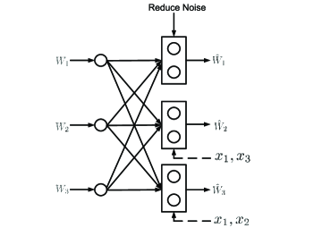
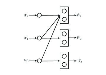
Figure 8: Genie-aided channel with noise reduction

Let a genie provide Receiver 2 with the side information containing the entire codewords $x_{1}$ and $x_{3}$. Then Receiver 2 can simply subtract out the interference from Transmitter 1 and 3 from its received signal. Similarly, $x_{1}$ and $x_{2}$ are given to Receiver 3 by a genie, so Receiver 3 can subtract out the interference from its received signal. Then we replace the original noise $\mathbf{Z}_{1}$ at Receiver 1 with $\mathbf{Z^{\prime}}_{1}$. These operations are summarized in Fig. 8. We end up with a many-to-one interference channel as shown in Fig. 8. It is obvious that the capacity region of this channel is an outer bound of the capacity region of the original interference channel. Now we will argue that on the genie-aided channel with noise reduction, Receiver 1 is able to decode all messages, hence giving the MAC bound. Consider any rate point in the capacity region of the genie-aided channel, so that each receiver can decode its message reliably. Receiver 1 can subtract $x_{1}$ from its own received signal after decoding it. The resulting channel is given by

$$\mathbf{Y^{\prime}}_{1} = \mathbf{H}_{12}x_{2}+\mathbf{H}_{13}x_{3}+\mathbf{Z}^{\prime}_{1}$$ (129)

$$\mathbf{Y^{\prime}}_{2} = \mathbf{H}_{22}x_{2}+\mathbf{Z}_{2}$$ (130)

$$\mathbf{Y^{\prime}}_{3} = \mathbf{H}_{33}x_{3}+\mathbf{Z}_{3}$$ (131)

Without loss of generality, we assume that $\|\mathbf{H}_{12}\|\geq\|\mathbf{H}_{13}\|$. Now we argue that Receiver 1 is able to decode $x_{2}$ by zero forcing $x_{3}$. It projects the received signal onto the direction that is orthogonal to $\mathbf{H}_{13}$. The resulting signal is

$$y_{1}=\sqrt{1-|c_{12,13}|^{2}}\|\mathbf{H}_{12}\|x_{2}+z_{1}$$ (132)

where $z_{1}\sim\mathcal{CN}(0,a_{1}^{2})$. (132) is equivalent to

$$y^{\prime}_{1}=x_{2}+z^{\prime}_{1}$$ (133)

where $y^{\prime}_{1}=\frac{y_{1}}{\sqrt{1-|c_{12,13}|^{2}}\|\mathbf{H}_{12}\|}$ and $z^{\prime}_{1}=\frac{z_{1}}{\sqrt{1-|c_{12,13}|^{2}}\|\mathbf{H}_{12}\|}\sim\mathcal{CN}(0,\frac{a^{2}_{1}}{(1-|c_{12,13}|^{2})\|\mathbf{H}_{12}\|^{2}})$. Note that at Receiver 2 the received signal (130) is equivalent to

$$y_{2}=x_{2}+z_{2}$$ (134)

where $z_{2}\sim\mathcal{CN}(0,1)$. Since $\frac{a_{1}}{\sqrt{1-|c_{12,13}|^{2}}\|\mathbf{H}_{12}\|}\leq 1$, (134) is more noisy than (133). This implies that Receiver 1 is able to decode $x_{2}$ since Receiver 2 can decode $x_{2}$. After decoding $x_{2}$, Receiver 1 can subtract it resulting in a clean channel from Transmitter 3:

$$y^{\prime\prime}_{1}=\|\mathbf{H}_{13}\|x_{3}+z^{\prime\prime}_{1}$$ (135)

where $z^{\prime\prime}_{1}\sim\mathcal{CN}(0,a_{1}^{2})$. (135) is equivalent to

$$\frac{y^{\prime\prime}_{1}}{\|\mathbf{H}_{13}\|}=x_{3}+\frac{z^{\prime\prime}_{1}}{\|\mathbf{H}_{13}\|}$$ (136)

where $\frac{z^{\prime\prime}_{1}}{\|\mathbf{H}_{13}\|}\sim\mathcal{CN}(0,\frac{a^{2}_{1}}{\|\mathbf{H}_{13}\|^{2}})$. Note that (131) is equivalent to

$$y_{3}=x_{3}+z_{3}$$ (137)

where $z_{3}\sim\mathcal{CN}(0,1)$. Since $\frac{a^{2}_{1}}{\|\mathbf{H}_{13}\|^{2}}\leq 1$, (137) is more noisy than (136). This implies that Receiver 1 is able to decode $x_{3}$ since Receiver 3 can decode $x_{3}$. As a result, Receiver 1 is able to decode both $x_{2}$ and $x_{3}$, hence giving the MAC bound.

By the same arguments, Receiver 2 and Receiver 3 can decode all messages if the noise at Receiver 2 and Receiver 3 are modified to $\mathbf{Z}_{2}^{\prime}$ and $\mathbf{Z}_{3}^{\prime}$, respectively. Therefore, the capacity region of the original interference channel is bounded above by the intersection of the capacity regions of the 3 MACs. ∎

A direct application of this outer bound is to establish the capacity region of the 3 user SIMO interference channel in strong interference regime, where each receiver can decode all messages.

Corollary 1

The capacity region of the 3 user SIMO Gaussian interference channel is the intersection of the MAC capacity regions of each receiver, if the following conditions are true:

$$(1-|c_{12,13}|^{2})\geq\min(\frac{1}{\|\mathbf{H}_{12}\|^{2}},\frac{1}{\|\mathbf{H}_{13}\|^{2}}),~{}~{}\min(\|\mathbf{H}_{12}\|,\|\mathbf{H}_{13}\|)\geq 1$$ (138)

$$(1-|c_{21,23}|^{2})\geq\min(\frac{1}{\|\mathbf{H}_{21}\|^{2}},\frac{1}{\|\mathbf{H}_{23}\|^{2}}),~{}~{}\min(\|\mathbf{H}_{21}\|,\|\mathbf{H}_{23}\|)\geq 1$$ (139)

$$(1-|c_{31,32}|^{2})\geq\min(\frac{1}{\|\mathbf{H}_{31}\|^{2}},\frac{1}{\|\mathbf{H}_{32}\|^{2}}),~{}~{}\min(\|\mathbf{H}_{31}\|,\|\mathbf{H}_{32}\|)\geq 1$$ (140)

Proof:

If (138), (139), (140) are satisfied, then $a_{1}=a_{2}=a_{3}=1$ in Theorem 5. The outer bound is the intersection of the MAC capacity regions of each receiver. Since this region is achieved by decoding all messages at each receiver, this region is the capacity region of the 3 user SIMO interference channel. ∎

Remark: The capacity region in Corollary 1 is also the capacity region of the 3 user SIMO Gaussian multicast channel, where each transmitter has a common message for all receivers.

VIII Conclusion

We characterize the capacity of a class of symmetric SIMO Gaussian interference channels within $\mathcal{O}(1)$. To get this result, we first generalize the El Gamal and Costa deterministic interference channel model to study a three user interference channel with multiple antenna nodes and find the capacity region of the proposed deterministic interference channel. Based on the insights provided by the deterministic channel, we characterize the generalized degrees of freedom of the $N+1$ user symmetric SIMO Gaussian interference channels with $N$ antennas at each receiver, which leads to the $\mathcal{O}(1)$ capacity characterization.

This work follows the idea of successive approximations of capacity of interference networks that have emerged throughout recent research on interference channel. Starting from degrees of freedom which is obtained in [12], we solve the GDOF problem and find the $\mathcal{O}(1)$ characterization and the exact capacity region for the strong interference regime. While we consider only the symmetric case in this paper, we believe the key ideas that emerge from this study can be used to solve the asymmetric case (as in the 2 user interference channel) as well in a similar manner. We suspect the extension will be extremely cumbersome due to the explosive growth in the number of parameters, but may be a useful exercise for a system designer to develop detailed insights into the problem of interference management for interference networks.

Finally, the SIMO setting is especially of interest for commonly occurring asymmetric communication scenarios where one end of the communication link, e.g. the base station is equipped with more antennas than the other, e.g. the user terminals. This work may provide useful insights for interference management schemes for such systems from an information theoretic perspective.

Appendix A Analysis of error probability for the 3 user deterministic interference channel

We only consider Receiver 1. The same analysis is applied to Receiver 2 and 3. Due to the symmetry of the code generation, the average probability of error averaged over all codes does not depend on the particular index that was sent. Thus, without loss of generality, we assume the message indexed by (1,1) is sent at Receiver 1, 2 and 3, i.e., $(j_{1},l_{1})=(j_{2},l_{2})=(j_{3},l_{3})=(1,1)$.

An error occurs if the correct codewords are not jointly typical with the received sequence, i.e.,

$$(X_{1}^{n}(1,1),V_{1}^{n}(1),V_{2}^{n}(1),V_{3}^{n}(1),Y_{1}^{n})\notin A_{n}^{\epsilon}.$$

Also, we have an error if the incorrect codewords from Transmitter 1 are jointly typical with the received sequence, i.e., $(X_{1}^{n}(\hat{j}_{1},\hat{l}_{1}),V_{1}^{n}(\hat{j}_{1}),V_{2}^{n}(\hat{j}_{2}),V_{3}^{n}(\hat{j}_{3}),Y_{1}^{n})\in A_{n}^{\epsilon}$ if $(\hat{j}_{1},\hat{l}_{1})\neq(1,1)$. Note that Receiver 1 is only interested in Transmitter 1’s message, so there is no error if the message from Transmitter 1 can be decoded correctly even the common messages from Transmitter 2 and 3 are decoded wrongly. Therefore, no error is declared if $(X_{1}^{n}(1,1),V_{1}^{n}(1),V_{2}^{n}(\hat{j}_{2}),V_{3}^{n}(\hat{j}_{3}),Y_{1}^{n})$ are jointly typical even $(\hat{j}_{2},\hat{j}_{3})\neq(1,1)$. Define the events

$$E_{j_{1}l_{1}j_{2}j_{3}}=\{(X_{1}^{n}(j_{1},l_{1}),V_{1}^{n}(j_{1}),V_{2}^{n}(j_{2}),V_{3}^{n}(j_{3}),Y_{1}^{n})\in A_{n}^{\epsilon}\}$$

Then the probability of error is

$$P_{e} = P\big{(}E_{1111}^{c}\bigcup\cup_{(j_{1},l_{1})\neq(1,1)}E_{j_{1}l_{1}j_{2}j_{3}}\big{)}$$

$$< P(E_{1111}^{c})+\sum_{j_{1}\neq 1,l_{1}\neq 1,j_{2}\neq 1,j_{3}\neq 1}P(E_{j_{1}l_{1}j_{2}j_{3}})+\sum_{j_{1}\neq 1,l_{1}\neq 1,j_{2}\neq 1,j_{3}=1}P(E_{j_{1}l_{1}j_{2}1})+\sum_{j_{1}\neq 1,l_{1}\neq 1,j_{2}=1,j_{3}\neq 1}P(E_{j_{1}l_{1}1j_{3}})$$

$$+\sum_{j_{1}\neq 1,l_{1}\neq 1,j_{2}=1,j_{3}=1}P(E_{j_{1}l_{1}11})+\sum_{j_{1}\neq 1,l_{1}=1,j_{2}\neq 1,j_{3}\neq 1}P(E_{j_{1}1j_{2}j_{3}})+\sum_{j_{1}\neq 1,l_{1}=1,j_{2}\neq 1,j_{3}=1}P(E_{j_{1}1j_{2}1})$$

$$+\sum_{j_{1}\neq 1,l_{1}=1,j_{2}=1,j_{3}\neq 1}P(E_{j_{1}11j_{3}})+\sum_{j_{1}\neq 1,l_{1}=1,j_{2}=1,j_{3}=1}P(E_{j_{1}111})+\sum_{j_{1}=1,l_{1}\neq 1,j_{2}\neq 1,j_{3}\neq 1}P(E_{1l_{1}j_{2}j_{3}})$$

$$+\sum_{j_{1}=1,l_{1}\neq 1,j_{2}\neq 1,j_{3}=1}P(E_{1l_{1}j_{2}1})+\sum_{j_{1}=1,l_{1}\neq 1,j_{2}=1,j_{3}\neq 1}P(E_{1l_{1}1j_{3}})+\sum_{j_{1}=1,l_{1}\neq 1,j_{2}=1,j_{3}=1}P(E_{1l_{1}11})$$

The first term is $\epsilon$ as $n\rightarrow\infty$. All other terms go to zero as $n\rightarrow\infty$, if the following constraints are satisfied:

$$R_{1c}+R_{1p}+R_{2c}+R_{3c} \leq I(X_{1},V_{2},V_{3};Y_{1})=H(Y_{1})$$

$$R_{1c}+R_{1p}+R_{2c} \leq I(X_{1},V_{2};Y_{1}|V_{3})=H(Y_{1}|V_{3})$$

$$R_{1c}+R_{1p}+R_{3c} \leq I(X_{1},V_{3};Y_{1}|V_{2})=H(Y_{1}|V_{2})$$

$$R_{1c}+R_{1p} \leq I(X_{1};Y_{1}|V_{2}V_{3})=H(Y_{1}|V_{2}V_{3})$$

$$R_{1c}+R_{2c}+R_{3c} \leq I(X_{1},V_{2},V_{3};Y_{1})=H(Y_{1})$$

$$R_{1c}+R_{2c} \leq I(X_{1},V_{2};Y_{1}|V_{3})=H(Y_{1}|V_{3})$$

$$R_{1c}+R_{3c} \leq I(X_{1},V_{3};Y_{1}|V_{2})=H(Y_{1}|V_{2})$$

$$R_{1c} \leq I(X_{1};Y_{1}|V_{2}V_{3})=H(Y_{1}|V_{2}V_{3})$$

$$R_{1p}+R_{2c}+R_{3c} \leq I(X_{1},V_{2},V_{3};Y_{1}|V_{1})=H(Y_{1}|V_{1})$$

$$R_{1p}+R_{2c} \leq I(X_{1},V_{2};Y_{1}|V_{1}V_{3})=H(Y_{1}|V_{1}V_{3})$$

$$R_{1p}+R_{3c} \leq I(X_{1},V_{3};Y_{1}|V_{1}V_{2})=H(Y_{1}|V_{1}V_{2})$$

$$R_{1p} \leq I(X_{1};Y_{1}|V_{1}V_{2}V_{3})=H(Y_{1}|V_{1}V_{2}V_{3})$$

$$R_{ip},R_{ic} \geq 0~{}\forall i=1,2,3$$

Reducing the redundant ones, we have

$$R_{1p}+R_{1c}+R_{2c}+R_{3c} \leq H(Y_{1})$$

$$R_{1c}+R_{1p}+R_{2c} \leq H(Y_{1}|V_{3})$$

$$R_{1c}+R_{1p}+R_{3c} \leq H(Y_{1}|V_{2})$$

$$R_{1p}+R_{2c}+R_{3c} \leq H(Y_{1}|V_{1})$$

$$R_{1p}+R_{2c} \leq H(Y_{1}|V_{1}V_{3})$$

$$R_{1p}+R_{3c} \leq H(Y_{1}|V_{1}V_{2})$$

$$R_{1c}+R_{1p} \leq H(Y_{1}|V_{2}V_{3})$$

$$R_{1p} \leq H(Y_{1}|V_{1}V_{2}V_{3})$$

$$R_{ip},R_{ic} \geq 0~{}\forall i=1,2,3$$

Receiver 2 (3) has similar constraints by swapping the indices 1 and 2 (3). All these conditions specify the achievable rate region for rate vector $(R_{1p},R_{2p},R_{3p},R_{1c},R_{2c},R_{3c})$.

Appendix B Proof for Lemma 5

Proof:

Let $\mathbf{S}_{j,\mathcal{B}}=\sum_{i\in\mathcal{B}}\mathbf{H}_{ji}x_{i}+\mathbf{Z}_{j}$ where $\mathcal{B}$ is a set of transmitters. And let $\mathcal{A}$ denote the set of all transmitters, i.e. $\mathcal{A}=\{1,2,\cdots,K\}$. The notation $\mathcal{A}\backslash\mathcal{B}$ means the complement of $\mathcal{B}$ in $\mathcal{A}$. First, let us consider $I(x_{1}^{n};\mathbf{Y}_{1}^{n})+I(x_{2}^{n};\mathbf{Y}_{2}^{n})$+$\cdots$+$I(x_{K-1}^{n};\mathbf{Y}_{K-1}^{n})$. By providing side information to receivers, we have

$$I(x_{1}^{n};\mathbf{Y}_{1}^{n}) \leq I(x_{1}^{n};\mathbf{Y}_{1}^{n},\mathbf{S}_{K,1}^{n})$$ (141)

$$= I(x_{1}^{n};\mathbf{S}_{K,1}^{n})+I(x_{1}^{n};\mathbf{Y}_{1}^{n}|\mathbf{S}_{K,1}^{n})$$

$$= h(\mathbf{S}_{K,1}^{n})-h(\mathbf{S}_{K,1}^{n}|x_{1}^{n})+h(\mathbf{Y}_{1}^{n}|\mathbf{S}_{K,1}^{n})-h(\mathbf{Y}_{1}^{n}|\mathbf{S}_{K,1}^{n},x_{1}^{n})$$

$$= h(\mathbf{S}_{K,1}^{n})-h(\mathbf{Z}_{K}^{n})+h(\mathbf{Y}_{1}^{n}|\mathbf{S}_{K,1}^{n})-h(\mathbf{S}_{1,\{2,3,\cdots,K\}}^{n})$$

For any $i=2,\ldots,K-1$,

$$I(x_{i}^{n};\mathbf{Y}_{i}^{n}) \leq I(x_{i}^{n};\mathbf{Y}_{i}^{n},\mathbf{S}_{K,\{1,2,\ldots,i\}}^{n},\mathbf{S}_{1,\mathcal{A}\backslash\{1,2,\ldots,i\}}^{n})$$ (142)

$$= I(x_{i}^{n};\mathbf{S}_{K,\{1,2,\ldots,i\}}^{n})+I(x_{i}^{n};\mathbf{Y}_{i}^{n},\mathbf{S}_{1,\mathcal{A}\backslash\{1,2,\ldots,i\}}^{n}|\mathbf{S}_{K,\{1,2,\ldots,i\}}^{n})$$

$$= h(\mathbf{S}_{K,\{1,2,\ldots,i\}}^{n})-h(\mathbf{S}_{K,\{1,2,\ldots,i\}}^{n}|x_{i}^{n})+I(x_{i}^{n};\mathbf{S}_{1,\mathcal{A}\backslash\{1,2,\ldots,i\}}^{n}|\mathbf{S}_{K,\{1,2,\ldots,i\}}^{n})$$

$$+I(x_{i}^{n};\mathbf{Y}_{i}^{n}|\mathbf{S}_{1,\mathcal{A}\backslash\{1,2,\ldots,i\}}^{n},\mathbf{S}_{K,\{1,2,\ldots,i\}}^{n})$$

$$= h(\mathbf{S}_{K,\{1,2,\ldots,i\}}^{n})-h(\mathbf{S}_{K,\{1,2,\ldots,i-1\}}^{n})+I(x_{i}^{n};\mathbf{Y}_{i}^{n}|\mathbf{S}_{1,\mathcal{A}\backslash\{1,2,\ldots,i\}}^{n},\mathbf{S}_{K,\{1,2,\ldots,i\}}^{n})$$

$$= h(\mathbf{S}_{K,\{1,2,\ldots,i\}}^{n})-h(\mathbf{S}_{K,\{1,2,\ldots,i-1\}}^{n})+h(\mathbf{Y}_{i}^{n}|\mathbf{S}_{1,\mathcal{A}\backslash\{1,2,\ldots,i\}}^{n},\mathbf{S}_{K,\{1,2,\ldots,i\}}^{n})$$

$$-h(\mathbf{Y}_{i}^{n}|\mathbf{S}_{1,\mathcal{A}\backslash\{1,2,\ldots,i\}}^{n},\mathbf{S}_{K,\{1,2,\ldots,i\}}^{n},x_{i}^{n})$$

$$\leq h(\mathbf{S}_{K,\{1,2,\ldots,i\}}^{n})-h(\mathbf{S}_{K,\{1,2,\ldots,i-1\}}^{n})+h(\mathbf{Y}_{i}^{n}|\mathbf{S}_{1,\mathcal{A}\backslash\{1,2,\ldots,i\}}^{n},\mathbf{S}_{K,\{1,2,\ldots,i\}}^{n})$$

$$-h(\mathbf{Y}_{i}^{n}|\mathbf{S}_{1,\mathcal{A}\backslash\{1,2,\ldots,i\}}^{n},\mathbf{S}_{K,\{1,2,\ldots,i\}}^{n},x_{\mathcal{A}}^{n})$$

$$= h(\mathbf{S}_{K,\{1,2,\ldots,i\}}^{n})-h(\mathbf{S}_{K,\{1,2,\ldots,i-1\}}^{n})+h(\mathbf{Y}_{i}^{n}|\mathbf{S}_{1,\mathcal{A}\backslash\{1,2,\ldots,i\}}^{n},\mathbf{S}_{K,\{1,2,\ldots,i\}}^{n})-h(\mathbf{Z}_{i}^{n})$$

Therefore,

$$I(x_{1}^{n};\mathbf{Y}_{1}^{n})+I(x_{2}^{n};\mathbf{Y}_{2}^{n})+\cdots+I(x_{K-1}^{n};\mathbf{Y}_{K-1}^{n})$$

$$\leq h(\mathbf{S}_{K,1}^{n})-h(\mathbf{Z}_{K}^{n})+h(\mathbf{Y}_{1}^{n}|\mathbf{S}_{K,1}^{n})-h(\mathbf{S}_{1,\{2,3,\cdots,K\}}^{n})$$

$$+\sum_{i=2}^{K-1}\big{(}h(\mathbf{S}_{K,\{1,2,\ldots,i\}}^{n})-h(\mathbf{S}_{K,\{1,2,\ldots,i-1\}}^{n})+h(\mathbf{Y}_{i}^{n}|\mathbf{S}_{1,\mathcal{A}\backslash\{1,2,\ldots,i\}}^{n},\mathbf{S}_{K,\{1,2,\ldots,i\}}^{n})-h(\mathbf{Z}_{i}^{n})\big{)}$$

$$= h(\mathbf{Y}_{1}^{n}|\mathbf{S}_{K,1}^{n})-h(\mathbf{S}_{1,\{2,3,\cdots,K\}}^{n})+\sum_{i=2}^{K-1}h(\mathbf{Y}_{i}^{n}|\mathbf{S}_{1,\mathcal{A}\backslash\{1,2,\ldots,i\}}^{n},\mathbf{S}_{K,\{1,2,\ldots,i\}}^{n})-\sum_{i=2}^{K-1}h(\mathbf{Z}_{i}^{n})-h(\mathbf{Z}_{K}^{n})$$

$$+h(\mathbf{S}_{K,1}^{n})+\sum_{i=2}^{K-1}\big{(}h(\mathbf{S}_{K,\{1,2,\ldots,i\}}^{n})-h(\mathbf{S}_{K,\{1,2,\ldots,i-1\}}^{n})\big{)}$$

$$= h(\mathbf{Y}_{1}^{n}|\mathbf{S}_{K,1}^{n})+\sum_{i=2}^{K-1}h(\mathbf{Y}_{i}^{n}|\mathbf{S}_{1,\mathcal{A}\backslash\{1,2,\ldots,i\}}^{n},\mathbf{S}_{K,\{1,2,\ldots,i\}}^{n})+h(\mathbf{S}_{K,\{1,2,\ldots,K-1\}}^{n})-h(\mathbf{S}_{1,\{2,3,\cdots,K\}}^{n})-\sum_{i=2}^{K}h(\mathbf{Z}_{i}^{n})$$

Similarly,

$$I(x_{K}^{n};\mathbf{Y}_{K}^{n})+I(x_{2}^{n};\mathbf{Y}_{2}^{n})+\cdots+I(x_{K-1}^{n};\mathbf{Y}_{K-1}^{n})$$

$$\leq h(\mathbf{Y}_{K}^{n}|\mathbf{S}_{1,K}^{n})+\sum_{i=2}^{K-1}h(\mathbf{Y}_{i}^{n}|\mathbf{S}_{K,\mathcal{A}\backslash\{K,2,\ldots,i\}}^{n},\mathbf{S}_{1,\{K,2,\ldots,i\}}^{n})+h(\mathbf{S}_{1,\{2,\ldots,K-1,K\}}^{n})-h(\mathbf{S}_{K,\{1,2,3,\cdots,K-1\}}^{n})-\sum_{i=1}^{K-1}h(\mathbf{Z}_{i}^{n})$$

Hence,

$$I(x_{1}^{n};\mathbf{Y}_{1}^{n})+2(I(x_{2}^{n};\mathbf{Y}_{2}^{n})+\cdots+I(x_{K-1}^{n};\mathbf{Y}_{K-1}^{n}))+I(x_{K}^{n};\mathbf{Y}_{K}^{n})$$

$$\leq h(\mathbf{Y}_{1}^{n}|\mathbf{S}_{K,1}^{n})+h(\mathbf{Y}_{K}^{n}|\mathbf{S}_{1,K}^{n})+\sum_{i=2}^{K-1}h(\mathbf{Y}_{i}^{n}|\mathbf{S}_{K,\mathcal{A}\backslash\{K,2,\ldots,i\}}^{n},\mathbf{S}_{1,\{K,2,\ldots,i\}}^{n})+\sum_{i=2}^{K-1}h(\mathbf{Y}_{i}^{n}|\mathbf{S}_{1,\mathcal{A}\backslash\{1,2,\ldots,i\}}^{n},\mathbf{S}_{K,\{1,2,\ldots,i\}}^{n})$$

$$-\sum_{i=1}^{K-1}h(\mathbf{Z}_{i}^{n})-\sum_{i=2}^{K}h(\mathbf{Z}_{i}^{n})$$

$$\leq n\big{(}h(\mathbf{Y}_{1}^{*}|\mathbf{S}_{K,1}^{*})+h(\mathbf{Y}_{K}^{*}|\mathbf{S}_{1,K}^{*})+\sum_{i=2}^{K-1}h(\mathbf{Y}_{i}^{*}|\mathbf{S}_{K,\mathcal{A}\backslash\{K,2,\ldots,i\}}^{*},\mathbf{S}_{1,\{K,2,\ldots,i\}}^{*})+\sum_{i=2}^{K-1}h(\mathbf{Y}_{i}^{*}|\mathbf{S}_{1,\mathcal{A}\backslash\{1,2,\ldots,i\}}^{*},\mathbf{S}_{K,\{1,2,\ldots,i\}}^{*})$$

$$-\sum_{i=1}^{K-1}h(\mathbf{Z}_{i})-\sum_{i=2}^{K}h(\mathbf{Z}_{i})\big{)}$$

where $\mathbf{Y}^{*}$ and $\mathbf{S}^{*}$ are the corresponding signals when $x_{i}\sim\mathcal{CN}(0,P_{i})$. This follows from Lemma 1 in [5]. Therefore, from Fano’s inequality, we have

$$R_{1}+2(R_{2}+\cdots+R_{K-1})+R_{K}-\epsilon_{n}$$

$$\leq \frac{1}{n}(I(x_{1}^{n};\mathbf{Y}_{1}^{n})+2(I(x_{2}^{n};\mathbf{Y}_{2}^{n})+\cdots+I(x_{K-1}^{n};\mathbf{Y}_{K-1}^{n}))+I(x_{K}^{n};\mathbf{Y}_{K}^{n}))$$

$$\leq h(\mathbf{Y}_{1}^{*}|\mathbf{S}_{K,1}^{*})+h(\mathbf{Y}_{K}^{*}|\mathbf{S}_{1,K}^{*})+\sum_{i=2}^{K-1}\big{(}h(\mathbf{Y}_{i}^{*}|\mathbf{S}_{K,\mathcal{A}\backslash\{K,2,\ldots,i\}}^{*},\mathbf{S}_{1,\{K,2,\ldots,i\}}^{*})+h(\mathbf{Y}_{i}^{*}|\mathbf{S}_{1,\mathcal{A}\backslash\{1,2,\ldots,i\}}^{*},\mathbf{S}_{K,\{1,2,\ldots,i\}}^{*})\big{)}$$

$$-2\sum_{i=2}^{K-1}h(\mathbf{Z}_{i})-h(\mathbf{Z}_{1})-h(\mathbf{Z}_{K})$$

Now we calculate each term in the above expression. First consider $h(\mathbf{Y}_{1}^{*}|\mathbf{S}_{K,1}^{*})$. Let $\Sigma_{\mathbf{Y}_{1}^{*}|\mathbf{S}_{K,1}^{*}}$ be the covariance matrix of $\mathbf{Y}_{1}^{*}|\mathbf{S}_{K,1}^{*}$. Then

$$h(\mathbf{Y}_{1}^{*}|\mathbf{S}_{K,1}^{*})=\log|\pi e\Sigma_{\mathbf{Y}_{1}^{*}|\mathbf{S}_{K,1}^{*}}|$$

where

$$\Sigma_{\mathbf{Y}_{1}^{*}|\mathbf{S}_{K,1}^{*}} = E[\mathbf{Y}_{1}^{*}\mathbf{Y}_{1}^{*\dagger}]-E[\mathbf{Y}_{1}^{*}\mathbf{S}_{K,1}^{*\dagger}]E[\mathbf{S}_{K,1}^{*}\mathbf{S}_{K,1}^{*\dagger}]^{-1}E[\mathbf{S}_{K,1}^{*}\mathbf{Y}_{1}^{*\dagger}]$$ (143)

$$= \mathbf{I}+\mathbf{H}_{11}P_{1}\mathbf{H}_{11}^{\dagger}+\sum_{i=2}^{K}\mathbf{H}_{1i}P_{i}\mathbf{H}_{1i}^{\dagger}-\mathbf{H}_{11}P_{1}\mathbf{H}_{K1}^{\dagger}(\mathbf{I}+\mathbf{H}_{K1}P_{1}\mathbf{H}_{K1}^{\dagger})^{-1}\mathbf{H}_{K1}P_{1}\mathbf{H}_{11}^{\dagger}$$ (144)

$$= \mathbf{I}+\sum_{i=2}^{K}\mathbf{H}_{1i}P_{i}\mathbf{H}_{1i}^{\dagger}+\mathbf{H}_{11}(P_{1}-P_{1}\mathbf{H}_{K1}^{\dagger}(\mathbf{I}+\mathbf{H}_{K1}P_{1}\mathbf{H}_{K1}^{\dagger})^{-1}\mathbf{H}_{K1}P_{1})\mathbf{H}_{11}^{\dagger}$$ (145)

$$\stackrel{{\scriptstyle(a)}}{{=}} \mathbf{I}+\sum_{i=2}^{K}\mathbf{H}_{1i}P_{i}\mathbf{H}_{1i}^{\dagger}+\mathbf{H}_{11}(\frac{1}{P_{1}}+\|\mathbf{H}_{K1}\|^{2})^{-1}\mathbf{H}_{11}^{\dagger}$$ (146)

where (a) follows from Woodbury matrix identity [16]. Therefore,

$$h(\mathbf{Y}_{1}^{*}|\mathbf{S}_{K,1}^{*})-h(\mathbf{Z}_{1})$$ (147)

$$= \log|\pi e(\mathbf{I}+\sum_{i=2}^{K}\mathbf{H}_{1i}P_{i}\mathbf{H}_{1i}^{\dagger}+\mathbf{H}_{11}(\frac{1}{P_{1}}+\|\mathbf{H}_{K1}\|^{2})^{-1}\mathbf{H}_{11}^{\dagger})|-N\log(\pi e)$$ (148)

$$= \log|\mathbf{I}+\sum_{i=2}^{K}\mathbf{H}_{1i}P_{i}\mathbf{H}_{1i}^{\dagger}+\frac{P_{1}}{1+P_{1}\|\mathbf{H}_{K1}\|^{2}}\mathbf{H}_{11}\mathbf{H}_{11}^{\dagger}|$$ (149)

Similarly,

$$h(\mathbf{Y}_{K}^{*}|\mathbf{S}_{1,K}^{*})-h(\mathbf{Z}_{K})=\log|\mathbf{I}+\sum_{i=1}^{K-1}\mathbf{H}_{Ki}P_{i}\mathbf{H}_{Ki}^{\dagger}+\frac{P_{K}}{1+P_{K}\|\mathbf{H}_{1K}\|^{2}}\mathbf{H}_{KK}\mathbf{H}_{KK}^{\dagger}|$$ (150)

Next, consider $h(\mathbf{Y}_{i}^{*}|\mathbf{S}_{1,\mathcal{A}\backslash\{1,2,\ldots,i\}}^{*},\mathbf{S}_{K,\{1,2,\ldots,i\}}^{*})$. We have

$$\mathbf{Y}_{i} = \underline{\mathbf{H}}_{i1}\underline{\mathbf{X}}_{1}+\underline{\mathbf{H}}_{i2}\underline{\mathbf{X}}_{2}+\mathbf{\mathbf{Z}}_{i}$$ (151)

$$\mathbf{S}_{K,\{1,2,\ldots,i\}}^{*} = \underline{\mathbf{H}}_{K1}\underline{\mathbf{X}}_{1}+\mathbf{\mathbf{Z}}_{K}$$ (152)

$$\mathbf{S}_{1,\mathcal{A}\backslash\{1,2,\ldots,i\}}^{*} = \underline{\mathbf{H}}_{12}\underline{\mathbf{X}}_{2}+\mathbf{\mathbf{Z}}_{1}$$ (153)

where

$$\underline{\mathbf{X}}_{1} = [x_{1}~{}x_{2}\cdots x_{i}]^{T}$$

$$\underline{\mathbf{X}}_{2} = [x_{i+1}~{}x_{i+2}\cdots x_{K}]^{T}$$

$$\underline{\mathbf{H}}_{i1} = [\mathbf{H}_{i1}~{}\mathbf{H}_{i2}\cdots\mathbf{H}_{ii}]$$

$$\underline{\mathbf{H}}_{i2} = [\mathbf{H}_{ii+1}~{}\mathbf{H}_{ii+2}\cdots\mathbf{H}_{iK}]$$

$$\underline{\mathbf{H}}_{K1} = [\mathbf{H}_{K1}~{}\mathbf{H}_{K2}\cdots\mathbf{H}_{Ki}]$$

$$\underline{\mathbf{H}}_{12} = [\mathbf{H}_{1i+1}~{}\mathbf{H}_{1i+2}\cdots\mathbf{H}_{1K}]$$

Hence,

$$h(\mathbf{Y}_{i}^{*}|\mathbf{S}_{K,\{1,2,\ldots,i\}}^{*},\mathbf{S}_{1,\mathcal{A}\backslash\{1,2,\ldots,i\}}^{*})=h(\underline{\mathbf{H}}_{i1}\underline{\mathbf{X}}_{1}+\underline{\mathbf{H}}_{i2}\underline{\mathbf{X}}_{2}+\mathbf{\mathbf{Z}}_{i}|\underline{\mathbf{H}}_{K1}\underline{\mathbf{X}}_{1}+\mathbf{\mathbf{Z}}_{K},\underline{\mathbf{H}}_{12}\underline{\mathbf{X}}_{2}+\mathbf{\mathbf{Z}}_{1})$$ (154)

Let $\Sigma$ be the covariance matrix of $\mathbf{Y}_{i}^{*}|\mathbf{S}_{K,\{1,2,\ldots,i\}}^{*},\mathbf{S}_{1,\mathcal{A}\backslash\{1,2,\ldots,i\}}^{*}$. We have

$$\Sigma = \mathbf{I}+\underline{\mathbf{H}}_{i1}\mathbf{\underline{P}}_{i1}\underline{\mathbf{H}}_{i1}^{\dagger}+\underline{\mathbf{H}}_{i2}\mathbf{\underline{P}}_{i2}\underline{\mathbf{H}}_{i2}^{\dagger}$$ (160)

$$-\left[\underline{\mathbf{H}}_{i1}\mathbf{\underline{P}}_{i1}\underline{\mathbf{H}}_{K1}^{\dagger}~{}\underline{\mathbf{H}}_{i2}\mathbf{\underline{P}}_{i2}\underline{\mathbf{H}}_{12}^{\dagger}\right]\left[\begin{array}[]{ccc}\mathbf{I}+\underline{\mathbf{H}}_{K1}\mathbf{\underline{P}}_{i1}\underline{\mathbf{H}}_{K1}^{\dagger}&{}\hfil&\mathbf{0}\\ \mathbf{0}&{}\hfil&\mathbf{I}+\underline{\mathbf{H}}_{12}\mathbf{\underline{P}}_{i2}\underline{\mathbf{H}}_{12}^{\dagger}\end{array}\right]^{-1}\left[\begin{array}[]{c}\underline{\mathbf{H}}_{K1}\mathbf{\underline{P}}_{i1}\underline{\mathbf{H}}_{i1}^{\dagger}\\ \underline{\mathbf{H}}_{12}\mathbf{\underline{P}}_{i2}\underline{\mathbf{H}}_{i2}^{\dagger}\end{array}\right]$$

$$= \mathbf{I}+\underline{\mathbf{H}}_{i1}\mathbf{\underline{P}}_{i1}\underline{\mathbf{H}}_{i1}^{\dagger}-\underline{\mathbf{H}}_{i1}\mathbf{\underline{P}}_{i1}\underline{\mathbf{H}}_{K1}^{\dagger}(\mathbf{I}+\underline{\mathbf{H}}_{K1}\mathbf{\underline{P}}_{i1}\underline{\mathbf{H}}_{K1}^{\dagger})^{-1}\underline{\mathbf{H}}_{K1}\mathbf{\underline{P}}_{i1}\underline{\mathbf{H}}_{i1}^{\dagger}$$ (162)

$$+\underline{\mathbf{H}}_{i2}\mathbf{\underline{P}}_{i2}\underline{\mathbf{H}}_{i2}^{\dagger}-\underline{\mathbf{H}}_{i2}\mathbf{\underline{P}}_{i2}\underline{\mathbf{H}}_{12}^{\dagger}(\mathbf{I}+\underline{\mathbf{H}}_{12}\mathbf{\underline{P}}_{i2}\underline{\mathbf{H}}_{12}^{\dagger})^{-1}\underline{\mathbf{H}}_{12}\mathbf{\underline{P}}_{i2}\underline{\mathbf{H}}_{i2}^{\dagger}$$

$$= \mathbf{I}+\underline{\mathbf{H}}_{i1}(\mathbf{\underline{P}}_{i1}-\mathbf{\underline{P}}_{i1}\underline{\mathbf{H}}_{K1}^{\dagger}(\mathbf{I}+\underline{\mathbf{H}}_{K1}\mathbf{\underline{P}}_{i1}\underline{\mathbf{H}}_{K1}^{\dagger})^{-1}\underline{\mathbf{H}}_{K1}\mathbf{\underline{P}}_{i1})\underline{\mathbf{H}}_{i1}^{\dagger}$$ (164)

$$+\underline{\mathbf{H}}_{i2}(\mathbf{\underline{P}}_{i2}-\mathbf{\underline{P}}_{i2}\underline{\mathbf{H}}_{12}^{\dagger}(\mathbf{I}+\underline{\mathbf{H}}_{12}\mathbf{\underline{P}}_{i2}\underline{\mathbf{H}}_{12}^{\dagger})^{-1}\underline{\mathbf{H}}_{12}\mathbf{\underline{P}}_{i2})\underline{\mathbf{H}}_{i2}^{\dagger}$$

$$\stackrel{{\scriptstyle(a)}}{{=}} \mathbf{I}+\underline{\mathbf{H}}_{i1}(\mathbf{\underline{P}}_{i1}^{-1}+\underline{\mathbf{H}}_{K1}^{\dagger}\underline{\mathbf{H}}_{K1})^{-1}\underline{\mathbf{H}}_{i1}^{\dagger}+\underline{\mathbf{H}}_{i2}(\mathbf{\underline{P}}_{i2}^{-1}+\underline{\mathbf{H}}_{12}^{\dagger}\underline{\mathbf{H}}_{12})^{-1}\underline{\mathbf{H}}_{i2}^{\dagger}$$ (165)

where (a) follows from Woodbury matrix identity [16] and

$$\underline{\mathbf{P}}_{i1}=\left[\begin{array}[]{ccc}P_{1}&\cdots&0\\ \vdots&\ddots&\vdots\\ 0&\cdots&P_{i}\end{array}\right]~{}~{}\underline{\mathbf{P}}_{i2}=\left[\begin{array}[]{ccc}P_{i+1}&\cdots&0\\ \vdots&\ddots&\vdots\\ 0&\cdots&P_{K}\end{array}\right]$$ (172)

Therefore,

$$h(\mathbf{Y}_{i}^{*}|\mathbf{S}_{K,\{1,2,\ldots,i\}}^{*},\mathbf{S}_{1,\mathcal{A}\backslash\{1,2,\ldots,i\}}^{*})-h(\mathbf{Z}_{i})$$ (173)

$$= \log|\pi e(\mathbf{I}+\underline{\mathbf{H}}_{i1}(\mathbf{\underline{P}}_{i1}^{-1}+\underline{\mathbf{H}}_{K1}^{\dagger}\underline{\mathbf{H}}_{K1})^{-1}\underline{\mathbf{H}}_{i1}^{\dagger}+\underline{\mathbf{H}}_{i2}(\mathbf{\underline{P}}_{i2}^{-1}+\underline{\mathbf{H}}_{12}^{\dagger}\underline{\mathbf{H}}_{12})^{-1}\underline{\mathbf{H}}_{i2}^{\dagger})|-N\log(\pi e)$$ (174)

$$= \log|\mathbf{I}+\underline{\mathbf{H}}_{i1}(\mathbf{\underline{P}}_{i1}^{-1}+\underline{\mathbf{H}}_{K1}^{\dagger}\underline{\mathbf{H}}_{K1})^{-1}\underline{\mathbf{H}}_{i1}^{\dagger}+\underline{\mathbf{H}}_{i2}(\mathbf{\underline{P}}_{i2}^{-1}+\underline{\mathbf{H}}_{12}^{\dagger}\underline{\mathbf{H}}_{12})^{-1}\underline{\mathbf{H}}_{i2}^{\dagger}|$$ (175)

Similarly, we have

$$h(\mathbf{Y}_{i}^{*}|\mathbf{S}_{1,\{K,2,\ldots,i\}}^{*},\mathbf{S}_{K,\mathcal{A}\backslash\{K,2,\ldots,i\}}^{*})-h(\mathbf{Z}_{i})$$ (176)

$$= \log|\mathbf{I}+\underline{\mathbf{H}}_{i3}(\mathbf{\underline{P}}_{i3}^{-1}+\underline{\mathbf{H}}_{13}^{\dagger}\underline{\mathbf{H}}_{13})^{-1}\underline{\mathbf{H}}_{i3}^{\dagger}+\underline{\mathbf{H}}_{i4}(\mathbf{\underline{P}}_{i4}^{-1}+\underline{\mathbf{H}}_{K4}^{\dagger}\underline{\mathbf{H}}_{K4})^{-1}\underline{\mathbf{H}}_{i4}^{\dagger}|$$ (177)

where

$$\underline{\mathbf{H}}_{i3} = [\mathbf{H}_{iK}~{}\mathbf{H}_{i2}\cdots\mathbf{H}_{ii}]$$

$$\underline{\mathbf{H}}_{i4} = [\mathbf{H}_{i1}~{}\mathbf{H}_{ii+1}\cdots\mathbf{H}_{iK-1}]$$

$$\underline{\mathbf{H}}_{13} = [\mathbf{H}_{1K}~{}\mathbf{H}_{12}\cdots\mathbf{H}_{1i}]$$

$$\underline{\mathbf{H}}_{K4} = [\mathbf{H}_{K1}~{}\mathbf{H}_{Ki+1}\cdots\mathbf{H}_{KK-1}]$$

$$\underline{\mathbf{P}}_{i3} = \left[\begin{array}[]{cccc}P_{K}&0&\cdots&0\\ 0&P_{2}&\cdots&0\\ \vdots&\vdots&\ddots&\vdots\\ 0&0&\cdots&P_{i}\end{array}\right]$$

$$\underline{\mathbf{P}}_{i4} = \left[\begin{array}[]{cccc}P_{1}&0&\cdots&0\\ 0&P_{i+1}&\cdots&0\\ \vdots&\vdots&\ddots&\vdots\\ 0&0&\cdots&P_{K-1}\end{array}\right]$$

Therefore,

$$R_{1}+2(R_{2}+\cdots+R_{K-1})+R_{K}$$

$$\leq\log|\mathbf{I}+\sum_{i=2}^{K}P_{i}\mathbf{H}_{1i}\mathbf{H}_{1i}^{\dagger}+\frac{P_{1}}{1+\|\mathbf{H}_{K1}\|^{2}P_{1}}\mathbf{H}_{11}\mathbf{H}_{11}^{\dagger}|$$

$$+\log|\mathbf{I}+\sum_{i=1}^{K-1}P_{i}\mathbf{H}_{Ki}\mathbf{H}_{Ki}^{\dagger}+\frac{P_{K}}{1+\|\mathbf{H}_{1K}\|^{2}P_{K}}\mathbf{H}_{KK}\mathbf{H}_{KK}^{\dagger}|$$

$$+\sum_{i=2}^{K-1}(\log|\mathbf{I}+\underline{\mathbf{H}}_{i1}(\underline{\mathbf{P}}_{i1}^{-1}+\mathbf{\underline{H}}_{K1}^{\dagger}\mathbf{\underline{H}}_{K1})^{-1}\mathbf{\underline{H}}_{i1}^{\dagger}+\underline{\mathbf{H}}_{i2}(\underline{\mathbf{P}}_{i2}^{-1}+\mathbf{\underline{H}}_{12}^{\dagger}\mathbf{\underline{H}}_{12})^{-1}\mathbf{\underline{H}}_{i2}^{\dagger}|$$

$$+\log|\mathbf{I}+\underline{\mathbf{H}}_{i3}(\underline{\mathbf{P}}_{i3}^{-1}+\mathbf{\underline{H}}_{13}^{\dagger}\mathbf{\underline{H}}_{13})^{-1}\mathbf{\underline{H}}_{i3}^{\dagger}+\underline{\mathbf{H}}_{i4}(\underline{\mathbf{P}}_{i4}^{-1}+\mathbf{\underline{H}}_{K4}^{\dagger}\mathbf{\underline{H}}_{K4})^{-1}\mathbf{\underline{H}}_{i4}^{\dagger}|)$$

∎

Appendix C proof for lemma 6

Proof:

Now we apply the bound in Lemma 5 to the $N+1$ user $1\times N$ symmetric SIMO interference channel. By replacing $\mathbf{H}_{ji}$ with $\sqrt{\rho^{\alpha}}\mathbf{H}_{ji}$ for $i\neq j$, $\mathbf{H}_{jj}$ with $\sqrt{\rho}\mathbf{H}_{jj}$ and setting $P_{i}=1$ in Lemma 5, we have

$$R_{1}+2(R_{2}+\cdots+R_{N})+R_{N+1}$$

$$\leq\log|\mathbf{I}+\sum_{i=2}^{N+1}\rho^{\alpha}\mathbf{H}_{1i}\mathbf{H}_{1i}^{\dagger}+\frac{\rho}{1+\rho^{\alpha}}\mathbf{H}_{11}\mathbf{H}_{11}^{\dagger}|$$ (180)

$$+\log|\mathbf{I}+\sum_{i=1}^{N}\rho^{\alpha}\mathbf{H}_{N+1i}\mathbf{H}_{N+1i}^{\dagger}+\frac{\rho}{1+\rho^{\alpha}}\mathbf{H}_{N+1N+1}\mathbf{H}_{N+1N+1}^{\dagger}|$$ (181)

$$+\sum_{i=2}^{N}(\log|\mathbf{I}+\rho^{\alpha}\underline{\mathbf{H}}_{i1}(\mathbf{I}+\rho^{\alpha}\underline{\mathbf{H}}_{N+11}^{\dagger}\underline{\mathbf{H}}_{N+11})^{-1}\underline{\mathbf{H}}_{i1}^{\dagger}+\rho^{\alpha}\underline{\mathbf{H}}_{i2}(\mathbf{I}+\rho^{\alpha}\underline{\mathbf{H}}_{12}^{\dagger}\underline{\mathbf{H}}_{12})^{-1}\underline{\mathbf{H}}_{i2}^{\dagger}|$$ (182)

$$+\log|\mathbf{I}+\rho^{\alpha}\underline{\mathbf{H}}_{i3}(\mathbf{I}+\rho^{\alpha}\underline{\mathbf{H}}_{13}^{\dagger}\underline{\mathbf{H}}_{13})^{-1}\underline{\mathbf{H}}_{i3}^{\dagger}+\rho^{\alpha}\underline{\mathbf{H}}_{i4}(\mathbf{I}+\rho^{\alpha}\underline{\mathbf{H}}_{N+14}^{\dagger}\underline{\mathbf{H}}_{N+14})^{-1}\underline{\mathbf{H}}_{i4}^{\dagger}|)$$ (183)

Note that here $\underline{\mathbf{H}}_{i1}=[\mathbf{H}_{i1}~{}\mathbf{H}_{i2}\cdots\sqrt{\rho^{1-\alpha}}\mathbf{H}_{ii}]$ and $\underline{\mathbf{H}}_{i3}=[\mathbf{H}_{iN+1}~{}\mathbf{H}_{i2}\cdots\sqrt{\rho^{1-\alpha}}\mathbf{H}_{ii}]$. Now let us calculate the degrees of freedom of the outer bound. Consider the first term.

$$\log|\mathbf{I}+\sum_{i=2}^{N+1}\rho^{\alpha}\mathbf{H}_{1i}\mathbf{H}_{1i}^{\dagger}+\frac{\rho}{1+\rho^{\alpha}}\mathbf{H}_{11}\mathbf{H}_{11}^{\dagger}|$$

$$\stackrel{{\scriptstyle(a)}}{{=}} (\max\{1-\alpha,\alpha\}+(N-1)\alpha)\log\rho+\mathcal{O}(1)$$

$$= \max\{1+(N-2)\alpha,N\alpha\}\log\rho+\mathcal{O}(1)$$ (185)

where $(a)$ follows from Lemma 1. Similarly, we have

$$\log|\mathbf{I}+\sum_{i=1}^{N}\rho^{\alpha}\mathbf{H}_{N+1i}\mathbf{H}_{N+1i}^{\dagger}+\frac{\rho}{1+\rho^{\alpha}}\mathbf{H}_{N+1N+1}\mathbf{H}_{N+1N+1}^{\dagger}|=\max\{1+(N-2)\alpha,N\alpha\}\log\rho+\mathcal{O}(1)$$ (186)

Next,

$$\log|\mathbf{I}+\rho^{\alpha}\underline{\mathbf{H}}_{i1}(\mathbf{I}+\rho^{\alpha}\underline{\mathbf{H}}_{N+11}^{\dagger}\underline{\mathbf{H}}_{N+11})^{-1}\underline{\mathbf{H}}_{i1}^{\dagger}+\rho^{\alpha}\underline{\mathbf{H}}_{i2}(\mathbf{I}+\rho^{\alpha}\underline{\mathbf{H}}_{12}^{\dagger}\underline{\mathbf{H}}_{12})^{-1}\underline{\mathbf{H}}_{i2}^{\dagger}|$$ (187)

$$= \log|\mathbf{I}+\rho^{\alpha}\underline{\mathbf{H}}_{i1}(\rho^{\alpha}\underline{\mathbf{H}}_{N+11}^{\dagger}\underline{\mathbf{H}}_{N+11})^{-1}\underline{\mathbf{H}}_{i1}^{\dagger}+\rho^{\alpha}\underline{\mathbf{H}}_{i2}(\rho^{\alpha}\underline{\mathbf{H}}_{12}^{\dagger}\underline{\mathbf{H}}_{12})^{-1}\underline{\mathbf{H}}_{i2}^{\dagger}|+\mathcal{O}(1)$$ (188)

$$= \log|\mathbf{I}+\underline{\mathbf{H}}_{i1}(\underline{\mathbf{H}}_{N+11}^{\dagger}\underline{\mathbf{H}}_{N+11})^{-1}\underline{\mathbf{H}}_{i1}^{\dagger}+\underline{\mathbf{H}}_{i2}(\underline{\mathbf{H}}_{12}^{\dagger}\underline{\mathbf{H}}_{12})^{-1}\underline{\mathbf{H}}_{i2}^{\dagger}|+\mathcal{O}(1)$$ (189)

$$\stackrel{{\scriptstyle(a)}}{{=}} \log|\mathbf{I}+\underline{\mathbf{H}}_{i1}\underline{\mathbf{H}}_{i1}^{\dagger}|+\mathcal{O}(1)$$ (190)

$$= \log|\mathbf{I}+\mathbf{H}_{i1}\mathbf{H}_{i1}^{\dagger}+\cdots+\mathbf{H}_{ii-1}\mathbf{H}_{ii-1}^{\dagger}+\rho^{1-\alpha}\mathbf{H}_{ii}\mathbf{H}_{ii}^{\dagger}|+\mathcal{O}(1)$$ (191)

$$= (1-\alpha)\log\rho+\mathcal{O}(1)$$ (192)

where ($a$) follows from the fact that $\underline{\mathbf{H}}_{i2}(\underline{\mathbf{H}}_{12}^{\dagger}\underline{\mathbf{H}}_{12})^{-1}\underline{\mathbf{H}}_{i2}^{\dagger}$ and $\underline{\mathbf{H}}_{N+11}^{\dagger}\underline{\mathbf{H}}_{N+11}$ are constant. Similarly, we have

$$\log|\mathbf{I}+\rho^{\alpha}\underline{\mathbf{H}}_{i3}(\mathbf{I}+\rho^{\alpha}\underline{\mathbf{H}}_{13}^{\dagger}\underline{\mathbf{H}}_{13})^{-1}\underline{\mathbf{H}}_{i3}^{\dagger}+\rho^{\alpha}\underline{\mathbf{H}}_{i4}(\mathbf{I}+\rho^{\alpha}\underline{\mathbf{H}}_{N+14}^{\dagger}\underline{\mathbf{H}}_{N+14})^{-1}\underline{\mathbf{H}}_{i4}^{\dagger}|$$ (193)

$$= (1-\alpha)\log\rho+\mathcal{O}(1)$$ (194)

From (185), (186), (192) and (194), we have

$$R_{1}+2(R_{2}+\cdots+R_{N})+R_{N+1}$$ (195)

$$\leq (2\max\{1+(N-2)\alpha,N\alpha\}+2(N-1)(1-\alpha))\log\rho+\mathcal{O}(1)$$ (196)

Hence,

$$d_{\text{sym}}(\alpha) \leq \frac{1}{2N}(2\max\{1+(N-2)\alpha,N\alpha\}+2(N-1)(1-\alpha))$$ (197)

$$= \max\{1-\frac{\alpha}{N},\frac{N-1}{N}+\frac{\alpha}{N}\}$$ (198)

∎

Appendix D Proof for Theorem 4

Proof:

We prove the theorem by calculating the difference between the inner bound and outer bound in different regimes. First, we state some equalities and inequalities which will be used repeatedly later. Define $\underline{\mathbf{H}}_{12}=[\mathbf{H}_{12}~{}\mathbf{H}_{13}]$. Consider

$$\log|\mathbf{I}+\rho^{\alpha}\underline{\mathbf{H}}_{12}\underline{\mathbf{H}}_{12}^{{\dagger}}|$$

$$= \log|\mathbf{I}+\rho^{\alpha}\underline{\mathbf{H}}_{12}^{{\dagger}}\underline{\mathbf{H}}_{12}|$$

$$= \log|\mathbf{I}+\rho^{\alpha}\left[\begin{array}[]{cc}1&c\\ c^{*}&1\end{array}\right]|$$ (202)

$$= \log(1+2\rho^{\alpha}+\rho^{2\alpha}-\rho^{2\alpha}|c|^{2})$$ (203)

$$= \log(1+2\rho^{\alpha}+\rho^{2\alpha}|\bar{c}|^{2})$$ (204)

where $|\bar{c}|^{2}=1-|c|^{2}$. If $\alpha=0$ in (D), then

$$\log|\mathbf{I}+\underline{\mathbf{H}}_{12}\underline{\mathbf{H}}_{12}^{{\dagger}}|=\log(3+|\bar{c}|^{2})\leq 2$$ (205)

We will use inequality:

$$\log|\mathbf{I}+\rho^{\alpha}\underline{\mathbf{H}}_{12}\underline{\mathbf{H}}_{12}^{{\dagger}}|<\log|\mathbf{I}+\mathbf{H}_{11}\mathbf{H}^{{\dagger}}_{11}+\rho^{\alpha}\underline{\mathbf{H}}_{12}\underline{\mathbf{H}}_{12}^{{\dagger}}|<\log|\mathbf{I}+\mathbf{H}_{11}\mathbf{H}^{{\dagger}}_{11}|+\log|\mathbf{I}+\rho^{\alpha}\underline{\mathbf{H}}_{12}\underline{\mathbf{H}}_{12}^{{\dagger}}|$$ (206)

Notice that this inequality is GDOF tight, i.e., the 3 parts are equal in terms of GDOF.

We present the outer bounds which will be used later. The first one is the single user bound:

$$R \leq \log(1+\rho)$$ (207)

The second bound is the two user bound. We apply Lemma 3 to a two user $1\times 2$ SIMO interference channel . It is obvious that this is also an outer bound for the 3 user SIMO interference channel. Then, we have

$$R_{1}+R_{2} \leq \log|\mathbf{I}+\rho^{\alpha}\mathbf{H}_{12}\mathbf{H}_{12}^{\dagger}+\rho\mathbf{H}_{11}\mathbf{H}_{11}^{\dagger}|+\log(1+\frac{\rho}{1+\rho^{\alpha}})$$ (208)

$$\Rightarrow R \leq \frac{1}{2}\log|\mathbf{I}+\rho^{\alpha}\mathbf{H}_{12}\mathbf{H}_{12}^{\dagger}+\rho\mathbf{H}_{11}\mathbf{H}_{11}^{\dagger}|+\frac{1}{2}\log(1+\frac{\rho}{1+\rho^{\alpha}})$$ (209)

where $R$ is the symmetric rate. Similarly,

$$R \leq \frac{1}{2}\log|\mathbf{I}+\rho^{\alpha}\mathbf{H}_{13}\mathbf{H}_{13}^{\dagger}+\rho\mathbf{H}_{11}\mathbf{H}_{11}^{\dagger}|+\frac{1}{2}\log(1+\frac{\rho}{1+\rho^{\alpha}})$$ (210)

The third bound is obtained by applying Lemma 5 to the 3 user symmetric SIMO interference channel. Then, we have

$$R_{1}+2R_{2}+R_{3} \leq \log|\mathbf{I}+\rho^{\alpha}\mathbf{\underline{H}}_{12}\mathbf{\underline{H}}_{12}^{\dagger}+\frac{\rho}{1+\rho^{\alpha}}\mathbf{H}_{11}\mathbf{H}_{11}^{\dagger}|+\log|\mathbf{I}+\rho^{\alpha}\underline{\mathbf{H}}_{32}\underline{\mathbf{H}}_{32}^{\dagger}+\frac{\rho}{1+\rho^{\alpha}}\mathbf{H}_{33}\mathbf{H}_{33}^{\dagger}|$$

$$+\log|\mathbf{I}+\rho^{\alpha}\underline{\mathbf{H}}_{21}(\mathbf{I}+\rho^{\alpha}\underline{\mathbf{H}}_{31}^{\dagger}\underline{\mathbf{H}}_{31})^{-1}\underline{\mathbf{H}}_{21}^{\dagger}+\frac{\rho^{\alpha}}{1+\rho^{\alpha}}\mathbf{H}_{23}\mathbf{H}_{23}^{\dagger}|$$

$$+\log|\mathbf{I}+\rho^{\alpha}\underline{\mathbf{H}}_{23}(\mathbf{I}+\rho^{\alpha}\underline{\mathbf{H}}_{13}^{\dagger}\underline{\mathbf{H}}_{13})^{-1}\underline{\mathbf{H}}_{23}^{\dagger}+\frac{\rho^{\alpha}}{1+\rho^{\alpha}}\mathbf{H}_{21}\mathbf{H}_{21}^{\dagger}|$$

where

$$\underline{\mathbf{H}}_{32} = [\mathbf{H}_{31}~{}\mathbf{H}_{32}]$$

$$\underline{\mathbf{H}}_{21} = [\mathbf{H}_{21}~{}\sqrt{\rho^{1-\alpha}}\mathbf{H}_{22}]$$

$$\underline{\mathbf{H}}_{31} = [\mathbf{H}_{31}~{}\mathbf{H}_{32}]$$

$$\underline{\mathbf{H}}_{23} = [\mathbf{H}_{23}~{}\sqrt{\rho^{1-\alpha}}\mathbf{H}_{22}]$$

$$\underline{\mathbf{H}}_{13} = [\mathbf{H}_{13}~{}\mathbf{H}_{12}]$$

We can loosen this bound a little such that it can be used to bound the gap between the outer bound and inner bound. Consider the third term in the above equation.

$$\log|\mathbf{I}+\rho^{\alpha}\underline{\mathbf{H}}_{21}(\mathbf{I}+\rho^{\alpha}\underline{\mathbf{H}}_{31}^{\dagger}\underline{\mathbf{H}}_{31})^{-1}\underline{\mathbf{H}}_{21}^{\dagger}+\frac{\rho^{\alpha}}{1+\rho^{\alpha}}\mathbf{H}_{23}\mathbf{H}_{23}^{\dagger}|$$ (211)

$$< \log|\mathbf{I}+\rho^{\alpha}\underline{\mathbf{H}}_{21}(\mathbf{I}+\rho^{\alpha}\underline{\mathbf{H}}_{31}^{\dagger}\underline{\mathbf{H}}_{31})^{-1}\underline{\mathbf{H}}_{21}^{\dagger}|+\log|\mathbf{I}+\frac{\rho^{\alpha}}{1+\rho^{\alpha}}\mathbf{H}_{23}\mathbf{H}_{23}^{\dagger}|$$ (212)

$$< \log|\mathbf{I}+\underline{\mathbf{H}}_{21}\underline{\mathbf{H}}_{21}^{\dagger}|+\log|\mathbf{I}+\frac{\rho^{\alpha}}{1+\rho^{\alpha}}\mathbf{H}_{23}\mathbf{H}_{23}^{\dagger}|$$ (213)

$$= \log|\mathbf{I}+\mathbf{H}_{21}\mathbf{H}_{21}^{\dagger}+\rho^{1-\alpha}\mathbf{H}_{22}\mathbf{H}_{22}^{\dagger}|+\log|\mathbf{I}+\frac{\rho^{\alpha}}{1+\rho^{\alpha}}\mathbf{H}_{23}\mathbf{H}_{23}^{\dagger}|$$ (214)

$$< \log|\mathbf{I}+\mathbf{H}_{21}\mathbf{H}_{21}^{\dagger}|+\log|\mathbf{I}+\rho^{1-\alpha}\mathbf{H}_{22}\mathbf{H}_{22}^{\dagger}|+\log|\mathbf{I}+\mathbf{H}_{23}\mathbf{H}_{23}^{\dagger}|$$ (215)

$$= \log(1+\rho^{1-\alpha})+2$$ (216)

Similarly,

$$\log|\mathbf{I}+\rho^{\alpha}\underline{\mathbf{H}}_{23}(\mathbf{I}+\rho^{\alpha}\underline{\mathbf{H}}_{13}^{\dagger}\underline{\mathbf{H}}_{13})^{-1}\underline{\mathbf{H}}_{23}^{\dagger}+\frac{\rho^{\alpha}}{1+\rho^{\alpha}}\mathbf{H}_{21}\mathbf{H}_{21}^{\dagger}|<\log(1+\rho^{1-\alpha})+2$$ (217)

Therefore,

$$R_{1}+2R_{2}+R_{3}$$

$$\leq \log|\mathbf{I}+\rho^{\alpha}\mathbf{\underline{H}}_{12}\mathbf{\underline{H}}_{12}^{\dagger}+\frac{\rho}{1+\rho^{\alpha}}\mathbf{H}_{11}\mathbf{H}_{11}^{\dagger}|+\log|\mathbf{I}+\rho^{\alpha}\underline{\mathbf{H}}_{32}\underline{\mathbf{H}}_{32}^{\dagger}+\frac{\rho}{1+\rho^{\alpha}}\mathbf{H}_{33}\mathbf{H}_{33}^{\dagger}|+2(2+\log(1+\rho^{1-\alpha}))$$

$$< \log|\mathbf{I}+\rho^{\alpha}\mathbf{\underline{H}}_{12}\mathbf{\underline{H}}_{12}^{\dagger}+\rho^{1-\alpha}\mathbf{H}_{11}\mathbf{H}_{11}^{\dagger}|+\log|\mathbf{I}+\rho^{\alpha}\underline{\mathbf{H}}_{32}\underline{\mathbf{H}}_{32}^{\dagger}+\rho^{1-\alpha}\mathbf{H}_{33}\mathbf{H}_{33}^{\dagger}|+2(2+\log(1+\rho^{1-\alpha}))$$

$$\stackrel{{\scriptstyle(a)}}{{=}} 2\log|\mathbf{I}+\rho^{\alpha}\mathbf{\underline{H}}_{12}\mathbf{\underline{H}}_{12}^{\dagger}+\rho^{1-\alpha}\mathbf{H}_{11}\mathbf{H}_{11}^{\dagger}|+2(2+\log(1+\rho^{1-\alpha}))$$

$$\Rightarrow R \leq \frac{1}{2}\log|\mathbf{I}+\rho^{\alpha}\mathbf{\underline{H}}_{12}\mathbf{\underline{H}}_{12}^{\dagger}+\rho^{1-\alpha}\mathbf{H}_{11}\mathbf{H}_{11}^{\dagger}|+\frac{1}{2}(2+\log(1+\rho^{1-\alpha}))$$ (218)

where (a) follows from the assumption about the symmetry of directions of channel vectors at different receivers.

The last bound is obtained by applying Lemma 3 to the 3 user symmetric SIMO interference channel. We have

$$R_{1}+R_{2}+R_{3}$$ (219)

$$\leq \log|\mathbf{I}+\rho^{\alpha}\underline{\mathbf{H}}_{12}\underline{\mathbf{H}}_{12}^{{\dagger}}+\rho\mathbf{H}_{11}\mathbf{H}_{11}^{{\dagger}}|-\log|\mathbf{I}+\rho^{\alpha}\underline{\mathbf{H}}_{12}\underline{\mathbf{H}}_{12}^{{\dagger}}|+2\log(1+\rho)+\log|\mathbf{I}+\frac{\rho^{\alpha}}{1+\rho}\underline{\mathbf{H}}_{12}\underline{\mathbf{H}}_{12}^{{\dagger}}|$$

$$< \log|\mathbf{I}+\rho^{\alpha}\underline{\mathbf{H}}_{12}\underline{\mathbf{H}}_{12}^{{\dagger}}+\rho\mathbf{H}_{11}\mathbf{H}_{11}^{{\dagger}}|-\log|\mathbf{I}+\rho^{\alpha}\underline{\mathbf{H}}_{12}^{{\dagger}}\underline{\mathbf{H}}_{12}|+2\log(1+\rho)+\log|\mathbf{I}+\rho^{\alpha-1}\underline{\mathbf{H}}_{12}^{{\dagger}}\underline{\mathbf{H}}_{12}|$$

$$\Rightarrow R \leq \frac{1}{3}\log|\mathbf{I}+\rho^{\alpha}\underline{\mathbf{H}}_{12}\underline{\mathbf{H}}_{12}^{{\dagger}}+\rho\mathbf{H}_{11}\mathbf{H}_{11}^{{\dagger}}|-\frac{1}{3}\log|\mathbf{I}+\rho^{\alpha}\underline{\mathbf{H}}_{12}\underline{\mathbf{H}}_{12}^{{\dagger}}|+\frac{2}{3}\log(1+\rho)+\frac{1}{3}\log|\mathbf{I}+\rho^{\alpha-1}\underline{\mathbf{H}}_{12}\underline{\mathbf{H}}_{12}^{{\dagger}}|$$

Since the achievable schemes are different for $\alpha>1$ and $0\leq\alpha\leq 1$, we consider two cases separately.

D-A $\alpha>1$

In this regime, the achievable scheme is to let each receiver decode all messages. Thus, the achievable rate region is the intersection of 3 MAC capacity regions, one at each receiver. Due to symmetry, consider the MAC at Receiver 1. The rate region is specified by

$$R_{1} \leq \log(1+\rho)$$ (221)

$$R_{2} \leq \log(1+\rho^{\alpha})$$ (222)

$$R_{3} \leq \log(1+\rho^{\alpha})$$ (223)

$$R_{1}+R_{2} \leq \log|\mathbf{I}+\rho\mathbf{H}_{11}\mathbf{H}_{11}^{{\dagger}}+\rho^{\alpha}\mathbf{H}_{12}\mathbf{H}_{12}^{\dagger}|$$ (224)

$$R_{1}+R_{3} \leq \log|\mathbf{I}+\rho\mathbf{H}_{11}\mathbf{H}_{11}^{{\dagger}}+\rho^{\alpha}\mathbf{H}_{13}\mathbf{H}_{13}^{\dagger}|$$ (225)

$$R_{2}+R_{3} \leq \log|\mathbf{I}+\rho^{\alpha}\mathbf{H}_{12}\mathbf{H}^{{\dagger}}_{12}+\rho^{\alpha}\mathbf{H}_{13}\mathbf{H}_{13}^{\dagger}|$$ (226)

$$R_{1}+R_{2}+R_{3} \leq \log|\mathbf{I}+\rho\mathbf{H}_{11}\mathbf{H}_{11}^{{\dagger}}+\rho^{\alpha}\mathbf{H}_{12}\mathbf{H}^{{\dagger}}_{12}+\rho^{\alpha}\mathbf{H}_{13}\mathbf{H}_{13}^{\dagger}|$$ (227)

The constraints at Receiver 2 (3) can be obtained by swapping the indices 1 and 2 (3). Due to symmetry of directions of channel vectors, the achievable symmetric rate is unaffected by swapping user indices. Thus, the achievable symmetric rate is specified by the following constraints:

$$R \leq \log(1+\rho)$$ (228)

$$R \leq \frac{1}{2}\log|\mathbf{I}+\rho\mathbf{H}_{11}\mathbf{H}_{11}^{{\dagger}}+\rho^{\alpha}\mathbf{H}_{12}\mathbf{H}_{12}^{\dagger}|$$ (229)

$$R \leq \frac{1}{2}\log|\mathbf{I}+\rho\mathbf{H}_{11}\mathbf{H}_{11}^{{\dagger}}+\rho^{\alpha}\mathbf{H}_{13}\mathbf{H}_{13}^{\dagger}|$$ (230)

$$R \leq \frac{1}{2}\log|\mathbf{I}+\rho^{\alpha}\mathbf{H}_{12}\mathbf{H}^{{\dagger}}_{12}+\rho^{\alpha}\mathbf{H}_{13}\mathbf{H}_{13}^{\dagger}|$$ (231)

$$R \leq \frac{1}{3}\log|\mathbf{I}+\rho\mathbf{H}_{11}\mathbf{H}_{11}^{{\dagger}}+\rho^{\alpha}\mathbf{H}_{12}\mathbf{H}^{{\dagger}}_{12}+\rho^{\alpha}\mathbf{H}_{13}\mathbf{H}_{13}^{\dagger}|$$ (232)

Next, we will calculate the gap between each inner bound and its corresponding outer bound. For (228), from the single user bound, the gap is 0. For (229), the corresponding outer bound is (209). Calculating the difference between (209) and (229), we have the gap

$$\frac{1}{2}\log(1+\frac{\rho}{1+\rho^{\alpha}})\leq 0.5$$ (233)

Similarly, the gap for (230) is no more than 0.5 bit/channel use. For (231), the corresponding outer bound is (218). Calculating the difference between (218) and (231), we have the gap

$$\frac{1}{2}\log|\mathbf{I}+\rho^{\alpha}\mathbf{\underline{H}}_{12}\mathbf{\underline{H}}_{12}^{\dagger}+\rho^{1-\alpha}\mathbf{H}_{11}\mathbf{H}_{11}^{\dagger}|+\frac{1}{2}(2+\log(1+\rho^{1-\alpha}))-\frac{1}{2}\log|\mathbf{I}+\rho^{\alpha}\mathbf{H}_{12}\mathbf{H}^{{\dagger}}_{12}+\rho^{\alpha}\mathbf{H}_{13}\mathbf{H}_{13}^{\dagger}|$$

$$< \frac{1}{2}\log|\mathbf{I}+\rho^{\alpha}\mathbf{\underline{H}}_{12}\mathbf{\underline{H}}_{12}^{\dagger}|+\frac{1}{2}\log|\mathbf{I}+\rho^{1-\alpha}\mathbf{H}_{11}\mathbf{H}_{11}^{\dagger}|+\frac{1}{2}(2+\log(1+\rho^{1-\alpha}))-\frac{1}{2}\log|\mathbf{I}+\rho^{\alpha}\mathbf{H}_{12}\mathbf{H}^{{\dagger}}_{12}+\rho^{\alpha}\mathbf{H}_{13}\mathbf{H}_{13}^{\dagger}|$$

$$= 1+\log(1+\rho^{1-\alpha})$$

$$\leq 2$$

For (232), the corresponding outer bound is (LABEL:gapouterbound3). Then the gap is

$$\frac{2}{3}\log(1+\rho)+\frac{1}{3}\log|\mathbf{I}+\rho^{\alpha-1}\underline{\mathbf{H}}_{12}\underline{\mathbf{H}}_{12}^{{\dagger}}|-\frac{1}{3}\log|\mathbf{I}+\rho^{\alpha}\underline{\mathbf{H}}_{12}\underline{\mathbf{H}}_{12}^{{\dagger}}|$$ (234)

$$= \frac{2}{3}\log(1+\rho)+\frac{1}{3}\log(1+2\rho^{\alpha-1}+\rho^{2\alpha-2}|\bar{c}|^{2})-\frac{1}{3}\log(1+2\rho^{\alpha}+\rho^{2\alpha}|\bar{c}|^{2})$$ (235)

$$= \frac{2}{3}\log(1+\rho)-\frac{2}{3}\log\rho+\frac{1}{3}\log(\rho^{2}+2\rho^{\alpha+1}+\rho^{2\alpha}|\bar{c}|^{2})-\frac{1}{3}\log(1+2\rho^{\alpha}+\rho^{2\alpha}|\bar{c}|^{2})$$ (236)

$$= \frac{2}{3}(\log(1+\rho)-\log\rho)+\frac{1}{3}\log\frac{\rho^{2}+2\rho^{\alpha+1}+\rho^{2\alpha}|\bar{c}|^{2}}{1+2\rho^{\alpha}+\rho^{2\alpha}|\bar{c}|^{2}}$$ (237)

$$< \frac{2}{3}(\log(1+\rho)-\log\rho)+\frac{1}{3}\log\frac{\rho^{2}+2\rho^{\alpha+1}+\rho^{2\alpha}|\bar{c}|^{2}}{\rho^{2\alpha}|\bar{c}|^{2}}$$ (238)

$$\stackrel{{\scriptstyle(a)}}{{<}} \frac{2}{3}+\frac{1}{3}\log\frac{4}{|\bar{c}|^{2}}$$ (239)

$$= \frac{4}{3}-\frac{1}{3}\log(|\bar{c}|^{2})$$ (240)

where (a) uses the fact that $|\bar{c}|^{2}\leq 1$ and $\alpha>1$.

D-B $0\leq\alpha\leq 1$

For this weak interference regime, the achievable scheme is the Han-Kobayashi type scheme. The achievable rate is the sum of the rate for the common messages and the rate for the private messages. Due to symmetric assumption, from (63), the achievable rate for the private message is

$$R_{p}=\log|\mathbf{I}+\underline{\mathbf{H}}_{12}\underline{\mathbf{H}}_{12}^{{\dagger}}+\rho^{1-\alpha}\mathbf{H}_{11}\mathbf{H}_{11}^{{\dagger}}|-\log|\mathbf{I}+\underline{\mathbf{H}}_{12}\underline{\mathbf{H}}_{12}^{{\dagger}}|$$

where $\underline{\mathbf{H}}_{12}=[\mathbf{H}_{12}~{}\mathbf{H}_{13}]$. For the achievable rate for the common message, it is the intersection of 3 MAC capacity regions, one at each receiver. The MAC constraints at Receiver 1 are

$$R_{1c}\leq\log|\mathbf{I}+\mathbf{H}_{13}\mathbf{H}^{{\dagger}}_{13}+\mathbf{H}_{12}\mathbf{H}_{12}^{\dagger}+\rho\mathbf{H}_{11}\mathbf{H}_{11}^{{\dagger}}|-\log|\mathbf{I}+\underline{\mathbf{H}}_{12}\underline{\mathbf{H}}_{12}^{{\dagger}}+\rho^{1-\alpha}\mathbf{H}_{11}\mathbf{H}_{11}^{{\dagger}}|$$ (241)

$$R_{2c}\leq\log|\mathbf{I}+\mathbf{H}_{13}\mathbf{H}^{{\dagger}}_{13}+\rho^{1-\alpha}\mathbf{H}_{11}\mathbf{H}_{11}^{{\dagger}}+\rho^{\alpha}\mathbf{H}_{12}\mathbf{H}_{12}^{\dagger}|-\log|\mathbf{I}+\underline{\mathbf{H}}_{12}\underline{\mathbf{H}}_{12}^{{\dagger}}+\rho^{1-\alpha}\mathbf{H}_{11}\mathbf{H}_{11}^{{\dagger}}|$$ (242)

$$R_{3c}\leq\log|\mathbf{I}+\mathbf{H}_{12}\mathbf{H}^{{\dagger}}_{12}+\rho^{1-\alpha}\mathbf{H}_{11}\mathbf{H}_{11}^{{\dagger}}+\rho^{\alpha}\mathbf{H}_{13}\mathbf{H}_{13}^{\dagger}|-\log|\mathbf{I}+\underline{\mathbf{H}}_{12}\underline{\mathbf{H}}_{12}^{{\dagger}}+\rho^{1-\alpha}\mathbf{H}_{11}\mathbf{H}_{11}^{{\dagger}}|$$ (243)

$$R_{1c}+R_{2c}\leq\log|\mathbf{I}+\mathbf{H}_{13}\mathbf{H}^{{\dagger}}_{13}+\rho\mathbf{H}_{11}\mathbf{H}_{11}^{{\dagger}}+\rho^{\alpha}\mathbf{H}_{12}\mathbf{H}_{12}^{\dagger}|-\log|\mathbf{I}+\underline{\mathbf{H}}_{12}\underline{\mathbf{H}}_{12}^{{\dagger}}+\rho^{1-\alpha}\mathbf{H}_{11}\mathbf{H}_{11}^{{\dagger}}|$$ (244)

$$R_{1c}+R_{3c}\leq\log|\mathbf{I}+\mathbf{H}_{12}\mathbf{H}^{{\dagger}}_{12}+\rho\mathbf{H}_{11}\mathbf{H}_{11}^{{\dagger}}+\rho^{\alpha}\mathbf{H}_{13}\mathbf{H}_{13}^{\dagger}|-\log|\mathbf{I}+\underline{\mathbf{H}}_{12}\underline{\mathbf{H}}_{12}^{{\dagger}}+\rho^{1-\alpha}\mathbf{H}_{11}\mathbf{H}_{11}^{{\dagger}}|$$ (245)

$$R_{2c}+R_{3c}\leq\log|\mathbf{I}+\rho^{\alpha}\mathbf{H}_{12}\mathbf{H}^{{\dagger}}_{12}+\rho^{1-\alpha}\mathbf{H}_{11}\mathbf{H}_{11}^{{\dagger}}+\rho^{\alpha}\mathbf{H}_{13}\mathbf{H}_{13}^{\dagger}|-\log|\mathbf{I}+\underline{\mathbf{H}}_{12}\underline{\mathbf{H}}_{12}^{{\dagger}}+\rho^{1-\alpha}\mathbf{H}_{11}\mathbf{H}_{11}^{{\dagger}}|$$ (246)

$$R_{1c}+R_{2c}+R_{3c}\leq\log|\mathbf{I}+\rho\mathbf{H}_{11}\mathbf{H}_{11}^{{\dagger}}+\rho^{\alpha}\mathbf{H}_{12}\mathbf{H}^{{\dagger}}_{12}+\rho^{\alpha}\mathbf{H}_{13}\mathbf{H}_{13}^{\dagger}|-\log|\mathbf{I}+\underline{\mathbf{H}}_{12}\underline{\mathbf{H}}_{12}^{{\dagger}}+\rho^{1-\alpha}\mathbf{H}_{11}\mathbf{H}_{11}^{{\dagger}}|$$ (247)

The constraints at Receiver 2 (3) can be obtained by swapping the indices 1 and 2 (3). Due to symmetry of directions of channel vectors, the achievable symmetric rate is unaffected by swapping user indices. Adding the the private message’s rate, we have the following achievable symmetric rate:

$$R \leq \log|\mathbf{I}+\mathbf{H}_{13}\mathbf{H}^{{\dagger}}_{13}+\mathbf{H}_{12}\mathbf{H}_{12}^{\dagger}+\rho\mathbf{H}_{11}\mathbf{H}_{11}^{{\dagger}}|-\log|\mathbf{I}+\underline{\mathbf{H}}_{12}\underline{\mathbf{H}}_{12}^{{\dagger}}|$$ (248)

$$R \leq \log|\mathbf{I}+\mathbf{H}_{13}\mathbf{H}^{{\dagger}}_{13}+\rho^{1-\alpha}\mathbf{H}_{11}\mathbf{H}_{11}^{{\dagger}}+\rho^{\alpha}\mathbf{H}_{12}\mathbf{H}_{12}^{\dagger}|-\log|\mathbf{I}+\underline{\mathbf{H}}_{12}\underline{\mathbf{H}}_{12}^{{\dagger}}|$$ (249)

$$R \leq \log|\mathbf{I}+\mathbf{H}_{12}\mathbf{H}^{{\dagger}}_{12}+\rho^{1-\alpha}\mathbf{H}_{11}\mathbf{H}_{11}^{{\dagger}}+\rho^{\alpha}\mathbf{H}_{13}\mathbf{H}_{13}^{\dagger}|-\log|\mathbf{I}+\underline{\mathbf{H}}_{12}\underline{\mathbf{H}}_{12}^{{\dagger}}|$$ (250)

$$R \leq \frac{1}{2}\log|\mathbf{I}+\mathbf{H}_{13}\mathbf{H}^{{\dagger}}_{13}+\rho\mathbf{H}_{11}\mathbf{H}_{11}^{{\dagger}}+\rho^{\alpha}\mathbf{H}_{12}\mathbf{H}_{12}^{\dagger}|+\frac{1}{2}\log|\mathbf{I}+\underline{\mathbf{H}}_{12}\underline{\mathbf{H}}_{12}^{{\dagger}}+\rho^{1-\alpha}\mathbf{H}_{11}\mathbf{H}_{11}^{{\dagger}}|-\log|\mathbf{I}+\underline{\mathbf{H}}_{12}\underline{\mathbf{H}}_{12}^{{\dagger}}|$$

$$R \leq \frac{1}{2}\log|\mathbf{I}+\mathbf{H}_{12}\mathbf{H}^{{\dagger}}_{12}+\rho\mathbf{H}_{11}\mathbf{H}_{11}^{{\dagger}}+\rho^{\alpha}\mathbf{H}_{13}\mathbf{H}_{13}^{\dagger}|+\frac{1}{2}\log|\mathbf{I}+\underline{\mathbf{H}}_{12}\underline{\mathbf{H}}_{12}^{{\dagger}}+\rho^{1-\alpha}\mathbf{H}_{11}\mathbf{H}_{11}^{{\dagger}}|-\log|\mathbf{I}+\underline{\mathbf{H}}_{12}\underline{\mathbf{H}}_{12}^{{\dagger}}|$$

$$R \leq \frac{1}{2}\log|\mathbf{I}+\rho^{\alpha}\mathbf{\underline{H}}_{12}\mathbf{\underline{H}}_{12}^{\dagger}+\rho^{1-\alpha}\mathbf{H}_{11}\mathbf{H}_{11}^{\dagger}|+\frac{1}{2}\log|\mathbf{I}+\mathbf{\underline{H}}_{12}\mathbf{\underline{H}}_{12}^{\dagger}+\rho^{1-\alpha}\mathbf{H}_{11}\mathbf{H}_{11}^{\dagger}|-\log|\mathbf{I}+\mathbf{\underline{H}}_{12}\mathbf{\underline{H}}_{12}^{\dagger}|$$ (253)

$$R \leq \frac{1}{3}\log|\mathbf{I}+\rho^{\alpha}\mathbf{\underline{H}}_{12}\mathbf{\underline{H}}_{12}^{\dagger}+\rho\mathbf{H}_{11}\mathbf{H}_{11}^{\dagger}|+\frac{2}{3}\log|\mathbf{I}+\mathbf{\underline{H}}_{12}\mathbf{\underline{H}}_{12}^{\dagger}+\rho^{1-\alpha}\mathbf{H}_{11}\mathbf{H}_{11}^{\dagger}|-\log|\mathbf{I}+\mathbf{\underline{H}}_{12}\mathbf{\underline{H}}_{12}^{\dagger}|$$ (254)

We will calculate the gap for each case.

For (248), the corresponding outer bound is the single user bound. Thus, the gap is

$$R_{\text{up}}-R_{\text{low}} = \log(1+\rho)-\log|\mathbf{I}+\mathbf{H}_{13}\mathbf{H}^{{\dagger}}_{13}+\mathbf{H}_{12}\mathbf{H}_{12}^{\dagger}+\rho\mathbf{H}_{11}\mathbf{H}_{11}^{{\dagger}}|+\log|\mathbf{I}+\underline{\mathbf{H}}_{12}\underline{\mathbf{H}}_{12}^{{\dagger}}|$$

$$< \log(1+\rho)-\log|\mathbf{I}+\rho\mathbf{H}_{11}\mathbf{H}_{11}^{{\dagger}}|+\log|\mathbf{I}+\underline{\mathbf{H}}_{12}\underline{\mathbf{H}}_{12}^{{\dagger}}|$$

$$\leq 2$$

For (249), the achievable rate can be bounded below as

$$R = \log|\mathbf{I}+\mathbf{H}_{13}\mathbf{H}^{{\dagger}}_{13}+\rho^{1-\alpha}\mathbf{H}_{11}\mathbf{H}_{11}^{{\dagger}}+\rho^{\alpha}\mathbf{H}_{12}\mathbf{H}_{12}^{\dagger}|-\log|\mathbf{I}+\underline{\mathbf{H}}_{12}\underline{\mathbf{H}}_{12}^{{\dagger}}|$$ (255)

$$> \log|\mathbf{I}+\rho^{1-\alpha}\mathbf{H}_{11}\mathbf{H}_{11}^{{\dagger}}+\rho^{\alpha}\mathbf{H}_{12}\mathbf{H}_{12}^{\dagger}|-\log|\mathbf{I}+\underline{\mathbf{H}}_{12}\underline{\mathbf{H}}_{12}^{{\dagger}}|$$ (256)

For the outer bound, by giving $x_{3}$ to Receiver 1 and 2, we essentially have a two user interference channel. We will use a sum rate bound for the 2 user MIMO interference channel derived in [15]. This bound is the generalization of the ETW bound to multiple antennas case.

$$R_{1}+R_{2}\leq h(\mathbf{Y}_{1}|\mathbf{S}_{21},x_{3})+h(\mathbf{Y}_{2}|\mathbf{S}_{12},x_{3})-h(\mathbf{Z}_{1})-h(\mathbf{Z}_{2})$$

where

$$\mathbf{S}_{21}=\sqrt{\rho^{\alpha}}\mathbf{H}_{21}x_{1}+\mathbf{Z}_{2}\quad\mathbf{S}_{12}=\sqrt{\rho^{\alpha}}\mathbf{H}_{12}x_{2}+\mathbf{Z}_{1}$$

Thus,

$$R_{1}+R_{2} \leq \log|\mathbf{I}+\rho^{\alpha}\mathbf{H}_{12}\mathbf{H}_{12}^{\dagger}+\frac{\rho}{1+\rho^{\alpha}}\mathbf{H}_{11}\mathbf{H}_{11}^{\dagger}|+\log|\mathbf{I}+\rho^{\alpha}\mathbf{H}_{21}\mathbf{H}_{21}^{\dagger}+\frac{\rho}{1+\rho^{\alpha}}\mathbf{H}_{22}\mathbf{H}_{22}^{\dagger}|$$ (257)

$$< \log|\mathbf{I}+\rho^{\alpha}\mathbf{H}_{12}\mathbf{H}_{12}^{\dagger}+\rho^{1-\alpha}\mathbf{H}_{11}\mathbf{H}_{11}^{\dagger}|+\log|\mathbf{I}+\rho^{\alpha}\mathbf{H}_{21}\mathbf{H}_{21}^{\dagger}+\rho^{1-\alpha}\mathbf{H}_{22}\mathbf{H}_{22}^{\dagger}|$$

$$\stackrel{{\scriptstyle(a)}}{{=}} 2\log|\mathbf{I}+\rho^{\alpha}\mathbf{H}_{12}\mathbf{H}_{12}^{\dagger}+\rho^{1-\alpha}\mathbf{H}_{11}\mathbf{H}_{11}^{\dagger}|$$ (258)

$$\Rightarrow R < \log|\mathbf{I}+\rho^{\alpha}\mathbf{H}_{12}\mathbf{H}_{12}^{\dagger}+\rho^{1-\alpha}\mathbf{H}_{11}\mathbf{H}_{11}^{\dagger}|$$ (259)

where (a) follows from the assumption about the symmetry of directions of channel vectors. By calculating the difference between (259) and (256), the gap is

$$\log|\mathbf{I}+\underline{\mathbf{H}}_{12}\underline{\mathbf{H}}_{12}^{{\dagger}}|\leq 2$$

Similarly, for (250) the gap is also 2 bits/channel use.

For (LABEL:achievablerate4), the achievable rate can be bounded below as

$$R = \frac{1}{2}\log|\mathbf{I}+\mathbf{H}_{13}\mathbf{H}^{{\dagger}}_{13}+\rho\mathbf{H}_{11}\mathbf{H}_{11}^{{\dagger}}+\rho^{\alpha}\mathbf{H}_{12}\mathbf{H}_{12}^{\dagger}|+\frac{1}{2}\log|\mathbf{I}+\underline{\mathbf{H}}_{12}\underline{\mathbf{H}}_{12}^{{\dagger}}+\rho^{1-\alpha}\mathbf{H}_{11}\mathbf{H}_{11}^{{\dagger}}|-\log|\mathbf{I}+\underline{\mathbf{H}}_{12}\underline{\mathbf{H}}_{12}^{{\dagger}}|$$

$$> \frac{1}{2}\log|\mathbf{I}+\rho\mathbf{H}_{11}\mathbf{H}_{11}^{{\dagger}}+\rho^{\alpha}\mathbf{H}_{12}\mathbf{H}_{12}^{\dagger}|+\frac{1}{2}\log|\mathbf{I}+\rho^{1-\alpha}\mathbf{H}_{11}\mathbf{H}_{11}^{{\dagger}}|-\log|\mathbf{I}+\underline{\mathbf{H}}_{12}\underline{\mathbf{H}}_{12}^{{\dagger}}|$$

The outer bound is (209). Therefore, the gap is

$$R_{\text{gap}} < \frac{1}{2}\log|\mathbf{I}+\rho^{\alpha}\mathbf{H}_{12}\mathbf{H}_{12}^{\dagger}+\rho\mathbf{H}_{11}\mathbf{H}_{11}^{\dagger}|+\frac{1}{2}\log(1+\frac{\rho}{1+\rho^{\alpha}})-\frac{1}{2}\log|\mathbf{I}+\rho\mathbf{H}_{11}\mathbf{H}_{11}^{{\dagger}}+\rho^{\alpha}\mathbf{H}_{12}\mathbf{H}_{12}^{\dagger}|$$

$$- \frac{1}{2}\log|\mathbf{I}+\rho^{1-\alpha}\mathbf{H}_{11}\mathbf{H}_{11}^{{\dagger}}|+\log|\mathbf{I}+\underline{\mathbf{H}}_{12}\underline{\mathbf{H}}_{12}^{{\dagger}}|$$

$$= \frac{1}{2}\log(1+\frac{\rho}{1+\rho^{\alpha}})-\frac{1}{2}\log(1+\rho^{1-\alpha})+\log|\mathbf{I}+\underline{\mathbf{H}}_{12}\underline{\mathbf{H}}_{12}^{{\dagger}}|$$

$$< 2$$

Similarly, for (LABEL:achievablerate5), the gap is 2 bits/channel user.

For (253), the achievable rate can be bounded below as

$$R = \frac{1}{2}\log|\mathbf{I}+\rho^{\alpha}\mathbf{\underline{H}}_{12}\mathbf{\underline{H}}_{12}^{\dagger}+\rho^{1-\alpha}\mathbf{H}_{11}\mathbf{H}_{11}^{\dagger}|+\frac{1}{2}\log|\mathbf{I}+\mathbf{\underline{H}}_{12}\mathbf{\underline{H}}_{12}^{\dagger}+\rho^{1-\alpha}\mathbf{H}_{11}\mathbf{H}_{11}^{\dagger}|-\log|\mathbf{I}+\mathbf{\underline{H}}_{12}\mathbf{\underline{H}}_{12}^{\dagger}|$$ (260)

$$> \frac{1}{2}\log|\mathbf{I}+\rho^{\alpha}\mathbf{\underline{H}}_{12}\mathbf{\underline{H}}_{12}^{\dagger}+\rho^{1-\alpha}\mathbf{H}_{11}\mathbf{H}_{11}^{\dagger}|+\frac{1}{2}\log(1+\rho^{1-\alpha})-\log|\mathbf{I}+\mathbf{\underline{H}}_{12}\mathbf{\underline{H}}_{12}^{\dagger}|$$

The outer bound is (218). Therefore, the gap is

$$R_{\text{gap}} < \frac{1}{2}\log|\mathbf{I}+\rho^{\alpha}\mathbf{\underline{H}}_{12}\mathbf{\underline{H}}_{12}^{\dagger}+\rho^{1-\alpha}\mathbf{H}_{11}\mathbf{H}_{11}^{\dagger}|+\frac{1}{2}(2+\log(1+\rho^{1-\alpha}))$$ (262)

$$-\frac{1}{2}\log|\mathbf{I}+\rho^{\alpha}\mathbf{\underline{H}}_{12}\mathbf{\underline{H}}_{12}^{\dagger}+\rho^{1-\alpha}\mathbf{H}_{11}\mathbf{H}_{11}^{\dagger}|-\frac{1}{2}\log(1+\rho^{1-\alpha})+\log|\mathbf{I}+\mathbf{\underline{H}}_{12}\mathbf{\underline{H}}_{12}^{\dagger}|$$

$$= 1+\log|\mathbf{I}+\mathbf{\underline{H}}_{12}\mathbf{\underline{H}}_{12}^{\dagger}|$$ (263)

$$\leq 3$$ (264)

Thus the gap for the symmetric capacity is 3 bits/channel use.

For (254), the achievable rate can be bounded below as

$$R = \frac{1}{3}\log|\mathbf{I}+\rho^{\alpha}\mathbf{\underline{H}}_{12}\mathbf{\underline{H}}_{12}^{\dagger}+\rho\mathbf{H}_{11}\mathbf{H}_{11}^{\dagger}|+\frac{2}{3}\log|\mathbf{I}+\mathbf{\underline{H}}_{12}\mathbf{\underline{H}}_{12}^{\dagger}+\rho^{1-\alpha}\mathbf{H}_{11}\mathbf{H}_{11}^{\dagger}|-\log|\mathbf{I}+\mathbf{\underline{H}}_{12}\mathbf{\underline{H}}_{12}^{\dagger}|$$ (265)

$$> \frac{1}{3}\log|\mathbf{I}+\rho^{\alpha}\mathbf{\underline{H}}_{12}\mathbf{\underline{H}}_{12}^{\dagger}+\rho\mathbf{H}_{11}\mathbf{H}_{11}^{\dagger}|+\frac{2}{3}\log|\mathbf{I}+\rho^{1-\alpha}\mathbf{H}_{11}\mathbf{H}_{11}^{\dagger}|-\log|\mathbf{I}+\mathbf{\underline{H}}_{12}\mathbf{\underline{H}}_{12}^{\dagger}|$$ (266)

The outer bound is (LABEL:gapouterbound3). Therefore, the gap is

$$R_{\text{up}}-R_{\text{low}}$$ (267)

$$< \frac{2}{3}\log(1+\rho)+\frac{1}{3}\log|\mathbf{I}+\rho^{\alpha-1}\underline{\mathbf{H}}_{12}^{{\dagger}}\underline{\mathbf{H}}_{12}|-\frac{1}{3}\log|\mathbf{I}+\rho^{\alpha}\underline{\mathbf{H}}_{12}^{{\dagger}}\underline{\mathbf{H}}_{12}|-\frac{2}{3}\log(1+\rho^{1-\alpha})+\log|\mathbf{I}+\mathbf{\underline{H}}_{12}\mathbf{\underline{H}}_{12}^{\dagger}|$$

$$< \frac{2}{3}\log(1+\rho)+\frac{1}{3}\log|\mathbf{I}+\underline{\mathbf{H}}_{12}^{{\dagger}}\underline{\mathbf{H}}_{12}|-\frac{1}{3}\log(1+2\rho^{\alpha}+\rho^{2\alpha}|\bar{c}|^{2})-\frac{2}{3}\log(1+\rho^{1-\alpha})+\log|\mathbf{I}+\mathbf{\underline{H}}_{12}\mathbf{\underline{H}}_{12}^{\dagger}|$$

$$= \frac{1}{3}\log\frac{(1+\rho)^{2}}{(1+2\rho^{\alpha}+\rho^{2\alpha}|\bar{c}|^{2})(1+\rho^{1-\alpha})^{2}}+\frac{4}{3}\log|\mathbf{I}+\underline{\mathbf{H}}_{12}^{{\dagger}}\underline{\mathbf{H}}_{12}|$$

$$< \frac{8}{3}-\frac{1}{3}\log(|\bar{c}|^{2})$$ (268)

Consider all cases, the gap is the maximum one, i.e., $\max\{3,\frac{8}{3}-\frac{1}{3}\log(|\bar{c}|^{2})\}$ bits/channel use. ∎

References

- [1] R.H. Etkin, D. Tse, H. Wang, “Gaussian Interference Channel Capacity to Within One Bit,” IEEE Transactions on Information Theory, vol. 54, No. 12, Dec. 2008
- [2] A. A. El Gamal and M. H. M. Costa, “The Capacity Region of a Class of Deterministic Interferenc Channels,” IEEE Transactions on Information Theory, vol. 28, No. 2, March 1982
- [3] A. Motahari and A. Khandani, “Capacity Bounds for the Gaussian Interference Channel,” in IEEE Transactions on Information theory, vol. 55, No.2, Feb. 2009.
- [4] X. Shang, G. Kramer, and B. Chen, “A new outer bound and the noisy-interference sum-rate capacity for Gaussian interference channels,” in IEEE Transactions on Information theory, vol. 55, No. 2, Feb. 2009.
- [5] V. Annapureddy and V. Veeravalli, “Gaussian interference networks: Sum capacity in the low interference regime and new outer bounds on the capacity region,” in Submitted to IEEE Transactions on Information Theory. arxiv:0802.3495, Feb 2008.
- [6] G. Bresler and D. Tse, “The two user Gaussian interference channel: A determinitic view,” Europ. Trans. Telecommun., vol. 19, no. 4, Jun. 2008.
- [7] G. Bresler, A. Parekh and D. Tse, “The approximate capacity of the many-to-one and one-to-many Gaussian interference channels,” in http://arxiv.org/abs/0809.3554, 2008.
- [8] V. Cadambe and S. Jafar, “Interference alignment and the degrees of freedom of the user interference channel,” IEEE Trans. on Information Theory, vol. 54, pp. 3425–3441, Aug. 2008.
- [9] V. Cadambe, S. Jafar and C. Wang, “Interference Alignment with Asymmetric Complex Signaling-Settling the Host-Madsen-Nostratinia Conjecture,” http://arxiv.org/abs/0904.0274, April 2009.
- [10] R. Etkin and E. Ordentlich, “On the Degrees of Freedom of the K User Gaussian Interference Channnel,” http://arxiv.org/abs/0901.1695, Jan. 2009.
- [11] S. Jafar and S. Vishwanath, “Generalized Degrees of Freedom of the Symmetric Gaussian User Interference Channel,” in arXiv:cs/0804.4489 [cs.IT], 2008.
- [12] T. Gou and S. Jafar, “Degrees of Freedom of the User MIMO Interference Channel,” Proceedings of 42nd Asilomar Conference on Signals, Systems and Computers, Oct 2008.
- [13] S. Avestimehr, S. Diggavi and D. Tse, “A deterministic approach to wireless relay networks,” in Proc. Allerton Conf. Communication, Control, and Computering, Monticello, IL, Sep. 2007.
- [14] I. Wang, D. Tse, “Gaussian Interference Channels with Multiple Receive Antennas: Capacity and Generalized Degrees of Freedom,” Proceedings of 46th Annual Allerton Conference on Communication, Control and Computing, 2008.
- [15] P.A. Parker, D.W. Bliss and V. Tarokh, “On the Degrees of Freedom of the MIMO Interference Channel,” 42nd Annual Conference on Infomration Sciences and Systems, 2008
- [16] Gene H. Golub and Charles F. Van Loan, “Matrix computations (3rd ed.)”, Johns Hopkins University Press, 1996