Attachment and detachment rate distributions in deep-bed filtration

Abstract

We study the transport and deposition dynamics of colloids in saturated porous media under unfavorable filtering conditions. As an alternative to traditional convection-diffusion or more detailed numerical models, we consider a mean-field description in which the attachment and detachment processes are characterized by an entire spectrum of rate constants, ranging from shallow traps which mostly account for hydrodynamic dispersivity, all the way to the permanent traps associated with physical straining. The model has an analytical solution which allows analysis of its properties including the long time asymptotic behavior and the profile of the deposition curves. Furthermore, the model gives rise to a filtering front whose structure, stability and propagation velocity are examined. Based on these results, we propose an experimental protocol to determine the parameters of the model.

I Introduction

Many processes in biological systems as well as in the chemical and petroleum industry involve the transport and filtration of particles in porous media with which they interact through various forcesIndakm-1987 ; Bloomfield-1999 ; Luhrmann-1999 ; Harvey-1991 . These interactions often result in particle adsorption and/or entrapment by the medium. Examples include filtration in the respiratory system, groundwater transport, in situ bioremediation, passage of white blood cells in brain blood vessels in the presence of jam-1 proteins, passage of viral particles in granular media, separation of species in chromatography, and gel permeation. The particle-medium interactions in these systems are not always optimal for particle retention. For example, the passage of groundwater through soil often happens under chemically unfavorable conditions, and as a result many captured particles (e.g., viruses and bacteria) may be released back to the solution. While filtration under favorable conditions has been studied and modeled extensivelyHerzig-1970 ; Tien-1979 ; Chiang-1985 ; Vigneswaran-1986 ; Vigneswaran-1988 ; Ghidaglia-1991 ; Tobiason-1994 ; Lee-Koplik-1996 ; Vigneswaran-1989 ; Jegatheesan-2005 , we are just beginning to understand the process occurring under unfavorable conditions.

Several models have been developed to describe the kinetics of particle filtration under unfavorable conditions. The most commonly used ones are, in essence, phenomenological mean-field models based on the convection-diffusion equation (CDE) [see Eq. (1) and Sec. II]. Typically, one models the dynamics of free particles in terms of the average drift velocity $v$ and the hydrodynamic dispersivity $\lambda$, while the net particle deposition rate $r_{d}$ accounting for particle attachment and detachment at trapping sites is a few-parameter function of local densities of free and trapped particles. For given filtering conditions, the parameters $\lambda$ and $v$ can be determined from a separate experiment with a tracer, while the coefficients of the function $r_{d}$ can be obtained by fitting Eq. (1) to the breakthrough curves.

Despite their attractive simplicity, it is widely accepted now that the phenomenological models at the mean-field level have significant problems. First, the depth dependent deposition curves for viruses and bacteria are often much steeper than it would be expected if the deposition rates were uniform throughout the substrateAbinger-1994 ; Baygents-1998 ; Simoni-1998 ; Bolster-1999 ; Bolster-2000 ; Redman-2001 ; Redman-2001B ; Tufenkji-2003 . This was commonly compensated by introducing the depth-dependent deposition rates. The problem was brought to light in Ref. li-2004 , where it was demonstrated that the steeper-than-expected deposition rates under unfavorable filtering conditions also exist for inert colloids.

Second, Bradford et al. Bradford-2002 ; Bradford-2003 pointed out that the usual mean-field models based on the CDE, accounting for dynamic dispersivity and attachment and detachment phenomena, cannot explain the shape of both the breakthrough curves and the subsequent filter flushing. In these experiments some particles were retained in the medium, and the authors argued for the need to include the straining (permanent capture of colloids) in the model. Even so, these models may still be insufficient to fit the experiments Yoon-2006 .

More elaborate models to describe deep-bed filtration have been proposed in Refs. Redner-2000 ; Hwang-2001 ; Kim-2006 ; shapiro-2007 . These models go beyond the mean-field description by simulating subsequent filter layers as a collection of multiply connected pipes with a wide distribution of radii, which results in a variation in flow speed and also of the attachment and detachment rates (even straining in some cases). The disadvantage of these models is that they are essentially computer based: it is difficult to gain an understanding of the qualitative properties of the solutions, without extensive simulations. Furthermore, the simulation results suffer from statistical uncertainties.

In the present work, we develop a minimalist mean-field model to investigate filtering under unfavorable conditions. The model accounts for both a convective flow and the primary attachment and detachment processes. Unlike the previous mean-field models of filtration, our model contains attachment sites (traps) with different detachment rates $B_{i}$ [see Eq. (32)], which allows an accurate modeling of the filtration dynamics over long-time periods for a broad range of inlet concentrations. Yet, the model admits exact analytical solutions for the profiles of the deposition and breakthrough curves which permit us to understand qualitatively the effect of the corresponding parameters and design a protocol for extracting them from experiment.

One of the advantages of our model is that the “shallow” short-lived traps represent the same effect as hydrodynamical dispersivity without generating unphysically fast moving particles or requiring an additional boundary condition at the inlet of the filter. The “deep” long-lived traps allow to correctly simulate long-time asymptotics of the released colloids in the effluent during a washout stage. The traps with intermediate detachment rates determine the most prominent features of breakthrough curves. The effect of every trap kind is to decrease the apparent drift velocity. As attachment and detachment rate constants depend on colloid size, we can also account for the apparent acceleration of larger particles without any microscopic description as in Ref. Scheibe-2003 . The particle-size distribution can be also used to analyze the steeper deposition profiles near the inlet of the filter Baygents-1998 ; Simoni-1998 ; Tufenkji-2003 ; li-2004 .

The paper is organized as follows. In Sec. II, we give a brief overview of colloid-transport experiments, CDE models, and their analytical solutions in simple cases. The linearized multirate convection-only filtration model is introduced in Sec. III. The model is characterized by a discrete or continuous trap-release-rate distribution; it is generally solved in quadratures, and completely in several special cases. The results support our argument that the hydrodynamic dispersivity can be traded for shallow traps. This serves as a basis for the exact solution of the full mean-field model for filtration under unfavorable conditions introduced in Sec. IV, where we show that a large class of such models can be mapped exactly back to the linearized ones and analyze their solutions, as well as the propagation velocity, structure, and stability of the filtering front. We suggest an experimental protocol to fit the parameters of the model in Sec. V and give our conclusions in Sec. VI.

II Background

II.1 Overview of colloid transport experiments

A typical setup of a colloid-transport experiment is shown in Fig. 1. A cylindrical column packed with sand or other filtering material is saturated with water running from top to bottom until the single-phase state (no trapped air bubbles) is achieved. At the end of this stage, colloidal particles are added to the incoming stream of water with both the concentration of the suspended particles and the flow rate kept constant over time $T$. This is sometimes followed by a filter washout stage in which clean water is pumped through the filter. The filtration processes are characterized by two relevant experimental quantities: the particle breakthrough and deposition profile curves. While breakthrough curve represents the concentration of effluent particles at the outlet of the column as a function of time, deposition curves illustrate the depth distribution of concentration of the particles retained throughout the column.

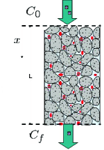
Figure 1: Schematic of experimental setup in the colloid-transport studies.

II.2 Convection-diffusion transport model

As the suspended particles move through the filtering column, each individual colloid follows its own trajectory. Consequently, even for small particles that are never trapped in the filter, the passage time through the column fluctuates. In the case of laminar flows with small Reynolds numbers and sufficiently small particles, which presumably follow the local velocity lines, the passage time scales inversely with the average flow velocity along the column $v$. The effects of the variation between the trajectories of particles as well as their speeds can be approximated by the velocity-dependent diffusion coefficient $D=\lambda v$, where $\lambda$ is the hydrodynamic dispersivity of the filtering medium. In comparison, the actual diffusion rate of colloids in experiments is negligibly small. Dispersivity is often obtained through tracer experiments in which the motion of the particles, i.e., salt ions, which move passively through the filter medium without being trapped, is traced as a function of time.

Overall, the dynamics of the suspended particles along the filter can be approximated by the mean-field CDE,

$$\frac{\partial C}{\partial t}+v\frac{\partial C}{\partial x}-\lambda v\frac{\partial^{2}C}{\partial x^{2}}=-r_{d},$$ (1)

where $C\equiv C(x,t)$ is the number of suspended particles per unit water volume averaged over the filter cross section at a given distance $x$ from the inlet and $r_{d}$ is the deposition rate which may include both attachment and detachment processes.

II.3 Issues with the CDE approximation

The diffusion approximation employed in Eq. (1) has two drawbacks which could seriously affect the resulting calculations if enough care is not used.

First, while the diffusion approximation works well to describe the concentration $C(x,t)$ of suspended particles in places where $C(x,t)$ is large, it seems to significantly overestimate the number of particles far downstream where $C(x,t)$ is expected to be small or zero. This is mainly due to the fact that the diffusion process allows for infinitely fast transport, albeit for a vanishingly small fraction of particles. In the simple case of tracer dynamics [$r_{d}=0$ in Eq. (1)], the general solutions as presented in Eqs. (6) and (7) are non-zero even at very large distances $x-vt\gg 2(\lambda vt)^{1/2}$. While in many instances this may not be crucial, the application of the model to, e.g., public health and water safety issues might trigger a false alert.

Second, for the filtering problem one expects the concentration $C(x,t)$ to be continuous, with the concentration downstream uniquely determined by that of the upstream. On the other hand, Eq. (1) contains second spatial derivative, which requires in addition to the knowledge of $C(x,t)$ at the inlet, $x=0$, another type of boundary condition to describe the concentration of particles along the column. This additional boundary condition could be, e.g., the spatial derivative $C^{\prime}(x,t)$ at the inlet, $x=0$, or the outlet, $x=L$ Lapidus-1952 ; Tufenkji-2003 , or the fixed value of the concentration at the outlet. We show below that fixing a derivative introduces an incontrollable error. On the other hand, we cannot introduce a boundary condition for the function $C(x,t)$ at the outlet, $x=L$, as this is precisely the quantity of interest to calculate.

The situation has an analogy in neutron physicsneutron-diffusion . While neutrons propagate diffusively within a medium, they move ballistically in vacuum. A correct calculation of the neutron flux requires a detailed simulation of the momentum distribution function within a few mean-free paths from the surface separating vacuum and the medium. In contrast to the filtration theory, for the case of neutron scattering, where the neutron distribution is stationary it is common to use an approximate boundary condition in terms of a “linear extrapolation distance” (the inverse logarithmic derivative of neutron density).

The CDE [see Eq. (1)] can be solved on a semi-infinite interval ($x_{\rm max}\gg L$) with setting $C^{\prime}(x,t)=0$ at $x_{\rm max}$ and calculating the value of $C(x,t)$ at $x=L$ as an approximation for the concentration of effluent particles. To illustrate this situation, we solve Eq. (1) for the case of tracer particles, where the deposition rate is set to zero, $r_{d}=0$. We consider a semi-infinite geometry with the initial condition $C(x,0)=0$ and a given concentration $C(0,t)$ at the inlet. The corresponding solution is presented in Sec. II.4. The spatial derivative at the boundary given in Eq. (9) is non-zero, time-dependent, and rather large at early stages of evolution when the diffusive current near the boundary is large. Therefore, setting an additional boundary condition for the derivative, e.g., $C^{\prime}(0,t)=0$, is unphysical.

On the other hand, the problem with the boundary condition far downstream, $C(x_{\rm max},t)=0$, $x_{\rm max}\gg L$, can be ill-defined numerically, as this condition is automatically satisfied to a good accuracy as long as the bulk of the colloids has not reached the end of the interval.

II.4 Tracer model

The simplest version of the convection-diffusion equation [Eq. (1)] applies to tracer particles where the deposition rate is set to zero, $r_{d}=0$,

$$\frac{\partial C}{\partial t}+v\frac{\partial C}{\partial x}-\lambda v\frac{\partial^{2}C}{\partial x^{2}}=0.$$ (2)

With the initial conditions, $C(x,0)=0$, the Laplace-transformed function $\tilde{C}\equiv\tilde{C}(x,p)$ obeys the equation

$$p\tilde{C}+v\tilde{C}^{\prime}-\lambda v\tilde{C}^{\prime\prime}=0,$$ (3)

where primes denote the spatial derivatives, $\tilde{C}^{\prime}\equiv\partial_{x}\tilde{C}(x,p)$. The solution to the above equation is $\tilde{C}\propto e^{\kappa x}$, with

$$\kappa_{\pm}={1\over 2\lambda}\pm\left({1\over 4\lambda^{2}}+{p\over\lambda v}\right)^{1/2}.$$ (4)

At semi-infinite interval $x>0$, only the solution with negative $\kappa=\kappa_{-}$ does not diverge at infinity. Given the Laplace-transformed concentration at the inlet, $\tilde{C}(0,p)$, we obtain

$$\tilde{C}(x,p)=\tilde{C}(0,p)\exp\left({x\over 2\lambda}-x\left[{1\over 4\lambda^{2}}+{p\over\lambda v}\right]^{1/2}\right).$$ (5)

The inverse Laplace transformation of the above equation is a convolution,

$$C(x,t)=\int_{0}^{t}dt^{\prime}\,C(0,t-t^{\prime})\,g(x,t^{\prime}),$$ (6)

with the tracer Green’s function (GF)

$$g(x,t)={x\over 2(\pi\lambda v)^{1/2}}{1\over t^{3/2}}\exp\left(-{(x-vt)^{2}\over 4\lambda vt}\right).$$ (7)

In the special case $C(0,t)=C_{0}=$const, the integration results

$$C=\frac{C_{0}}{2}\left(1+\mathop{\rm erf}\left[\frac{tv-x}{2({tv\lambda})^{1/2}}\right]+e^{x/\lambda}\mathop{\rm erfc}\left[\frac{tv+x}{2({tv\lambda})^{1/2}}\right]\right),$$ (8)

where $\mathop{\rm erfc}(z)\equiv 1-\mathop{\rm erf}(z)$ is the complementary error function.

We note that the spatial derivative of the solution of Eq. (8) at $x=0$ is different from zero. Indeed, it depends on time and is divergent at small $t$, implying an unphysically large diffusive component of the particle current,

$$C^{\prime}(0,t)=\frac{C_{0}}{2}\left({\mathop{\rm erfc}\left(\alpha\right)\over 2\lambda}-{e^{-\alpha^{2}}\over(\pi tv\lambda)^{1/2}}\right),\quad\alpha^{2}\equiv{tv\over 4\lambda}.$$ (9)

In the presence of the straining term, $r_{d}=A_{0}N_{0}C$ in Eq. (1), the GF can be obtained from Eq. (7) by introducing exponential decay with the rate $A_{0}N_{0}$,

$$g(x,t)={x\over 2(\pi\lambda v)^{1/2}}\,{e^{-A_{0}N_{0}t}\over t^{3/2}}\exp\left(-{(x-vt)^{2}\over 4\lambda vt}\right).$$ (10)

Note that we wrote the straining rate as a product of the capture rate $A_{0}$ by infinite-capacity “permanent” traps with the concentration $N_{0}$ per unit volume of water. Such a factorization is convenient for the non-linear model presented later in Sec. IV. The same notations are employed throughout this work for consistency.

III Linearized mean-field filtration model

In this section we discuss the linearized convection-only multitrap filtration model, a variant of the multirate CDE model first proposed in Ref. Haggerty-1995 . Our model is characterized by a (possibly continuous) density of traps as a function of detachment rate [see Eq. (23)]. Generically, continuous trap distribution leads to non-exponential (e.g., power-law) asymptotic forms of the concentration in the effluent on the washout stage.

The main purpose of this section is to demonstrate that “shallow” traps with large detachment rates have the same effect as the hydrodynamic dispersivity in CDE. In addition, the obtained exact solutions will be used in Sec. IV as a basis for the analysis of the full non-linear mean-field model for filtration under unfavorable conditions.

III.1 Shallow traps as a substitute for diffusion

To rectify the problems with the diffusion approximation noted previously, we suggest an alternative approach for the propagation of particles through the filtering medium. Instead of considering the drift with an average velocity with symmetric diffusion-like deviations accounting for dispersion of individual trajectories, we consider the convective motion with the maximum velocity $v$. The random twists and turns delaying the individual trajectories are accounted for by introducing Poissonian traps which slow down the passage of the majority of the particles through the column. In the simplest case suitable for tracer particles, the relevant kinetic equations read as follows:

$$\dot{C}+vC^{\prime}+N_{1}\dot{n}_{1}=0,\quad\dot{n}_{1}=A_{1}C-B_{1}n_{1},$$ (11)

with $n_{1}\equiv n_{1}(x,t)$ as the auxiliary variable describing the average number of particles in a trap, $N_{1}$ as the number of traps per unit water volume, $A_{1}$ as the trapping rate, and $B_{1}$ as the release rate. The particular normalization of the coefficients is chosen to simplify the formulation of models with traps subject to saturation in Sec. IV.

To simulate dispersivity where all time scales are inversely proportional to propagation velocity, we must choose both $A_{1}$ and $B_{1}$ proportional to $v$. The corresponding parameter $\sigma$ in $A_{1}\equiv\sigma v$ has a dimension of area and can be viewed as a trapping cross section. The length $\ell$ in the release rate $B_{1}\equiv v/\ell$ can be viewed as a characteristic size of a stagnation region. On general grounds we expect $\sigma\propto\ell^{2}$ with $\ell$ on the order of the grain size.

III.2 Single-trap model with straining.

To illustrate how shallow traps can provide for dispersivity in convection-only models, let us construct the exact solution of Eq. (11). In fact, it is convenient to consider a slightly generalized model with the addition of straining,

$$\dot{C}+vC^{\prime}+N_{1}\dot{n}_{1}=-A_{0}N_{0}C,\quad\dot{n}_{1}=A_{1}C-B_{1}n_{1}.$$ (12)

With zero initial conditions the Laplace transformation gives for $\tilde{C}\equiv\tilde{C}(x,p)$,

$$\left(p+A_{0}N_{0}+{A_{1}N_{1}p\over p+B_{1}}\right)\tilde{C}+v\tilde{C}^{\prime}=0.$$ (13)

The boundary value for Laplace-transformed $C(x,t)$ at the inlet is given by $\tilde{C}(0,p)$. With initially clean filter, $C(x,0)=n(x,0)=0$, and a given free particle concentration $C(0,t)$ at the inlet, the solution to the linear one-trap convection-only model with straining [Eq. (12)] is a convolution of the form presented in Eq. (6) with the following GF endnote :

$$g(x,t) = e^{-\beta x/v-B_{1}(t-x/v)}\Biggl{\{}\delta\left(t-{x}/{v}\right)$$ (14)

$$+\theta(t-x/v)\frac{(A_{1}N_{1}B_{1}x)^{1/2}}{({tv-x})^{1/2}}I_{1}(\zeta_{t})\Biggr{\}},$$

where $\beta\equiv A_{0}N_{0}+A_{1}N_{1}$ is the clean-bed trapping rate, $\theta(z)$ is the Heaviside step-function, and $I_{1}(\zeta_{t})$ is the modified Bessel function of the first kind with the argument

$$\zeta_{t}\equiv{2\over v}\left[A_{1}N_{1}B_{1}(tv-x)x\right]^{1/2}.$$ (15)

The singular term with the $\delta$ function $\delta(t-x/v)$ in Eq. (14) represents the particles at the leading edge which propagate freely with the maximum velocity $v$ without ever being trapped. The corresponding weight $\exp(-\beta x/v)$ decreases exponentially with the distance from the origin.

Sufficiently far from both the origin and from the leading edge, where the argument $\zeta_{t}$ [Eq. (15)] of the Bessel function is large, we can use the asymptotic form,

$$I_{1}(\zeta)={1\over(2\pi\zeta)^{1/2}}e^{\zeta}\left[1+\mathcal{O}(\zeta^{-1})\right],\mbox{Re}\,\zeta>0.$$ (16)

Subsequently, Eq. (14) becomes

$$g(x,t)\approx e^{-A_{0}N_{0}x/v}{B_{1}\xi^{1/4}\over 2\pi^{1/2}\tau^{3/4}}\exp-(\sqrt{\xi}-\sqrt{\tau})^{2},$$ (17)

where $\tau\equiv B_{1}(t-x/v)$ is the dimensionless retarded time in units of the release rate, and $\xi\equiv A_{1}N_{1}x/v$ is the dimensionless distance from the origin in units of the trapping mean free path.

The correspondence with the GF in Eq. (10) for the CDE with linear straining [or Eq. (7) for the CDE tracer model in the case of no permanent traps, $N_{0}=0$] can be recovered from Eq. (17) by expanding the square roots in the exponent around its maximum at $\xi=\tau$, or $x=v_{0}t$, with the effective velocity $v_{0}=vB_{1}/(B_{1}+N_{1}A_{1})$. Specifically, suppressing the prefactor due to straining, [$N_{0}=0$ in Eq. (17)], we obtain for the asymptotic form of the exponent at large $t$,

$$g(x,t)\propto\exp-{(x-v_{0}t)^{2}\over 4\lambda_{0}v_{0}t},$$ (18)

with the effective dispersivity coefficient [cf. Eq. (7)]

$$\lambda_{0}=v{N_{1}A_{1}\over(N_{1}A_{1}+B_{1})^{2}}.$$ (19)

The approximation is expected to be good as long as both $x$ and $t$ are large compared to the width of the bell-shaped maximum.

The actual shapes of the corresponding GFs, Eqs. (7) and (14) in the absence of permanent traps, $N_{0}=0$, are compared in Fig. 2. While the shape differences are substantial at small $t$, they disappear almost entirely at later times.

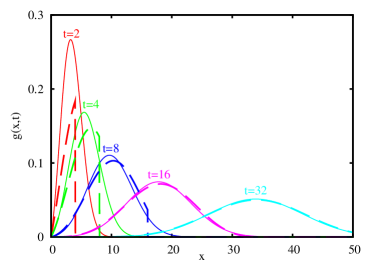
Figure 2: (Color online) Comparison of the spatial dependence of the GFs for the tracer model implemented as the convection-diffusion equation [Eq. (1)] with $r_{d}=0$ (solid lines) and the single-trap convection model [Eq. (11)] (dashed lines). Specifically, we plot Eq. (7) and the regular part of Eq. (14) with $N_{0}=0$, using identical values of $v=v_{0}=1$ and $\lambda=\lambda_{0}=1$ and the release rate $B_{1}=1/2$ (half the maximum value at these parameters) at $t=2$, $4$, $8$, $16$, $32$. Once the maximum is sufficiently far from the origin, the two GFs are virtually identical (see Sec. III.2).

III.3 Multitrap convection-only model

Even though the solutions of the single-trap model correspond to those of the CDE [Eq. (2)], the model presented in Eq. (12) is clearly too simple to accurately describe filtration under conditions where trapped particles can be subsequently released. At the very least, in addition to straining and “shallow” traps that account for the dispersivity, describing the experimentsBradford-2002 ; Bradford-2003 requires another set of “deeper” traps with a smaller release rate.

More generally, consider a linear model with $m$ types of traps differing by the rate coefficients $A_{i}$, $B_{i}$,

$$\dot{C}+vC^{\prime}+\sum_{i=1}^{m}N_{i}\dot{n}_{i}=0,\quad\dot{n}_{i}=A_{i}C-B_{i}n_{i}.$$ (20)

The corresponding solution can be obtained in quadratures in terms of the Laplace transformation. With the initial condition, $C(x,0)=n_{i}(x,0)=0$ and a given time-dependent concentration at the inlet, $C(0,t)=C_{0}(t)$, the result for $C(x,t)$ is a convolution of the form presented in Eq. (6) with the GF given by the inverse Laplace transformation formula,

$$g(x,t)=\int_{c-i\infty}^{c+i\infty}{dp\over 2\pi i}e^{\,\textstyle p\,[t-x/v-x\Sigma(p)/v]},$$ (21)

with the response function

$$\Sigma(p)\equiv\sum_{i=1}^{m}{A_{i}N_{i}\over p+B_{i}}=\int{dB\,\rho(B)\over p+B}.$$ (22)

Here we introduced the effective density of traps,

$$\rho(B)\equiv\sum_{i=1}^{m}A_{i}N_{i}\delta(B-B_{i}),$$ (23)

corresponding to various release rates.

The general structure of the concentration profile can be read off directly from Eq. (21). It gives zero for $t<x/v$, consistent with the fact that $v$ is the maximum propagation velocity in Eq. (20). The structure of the leading-edge singularity (the amplitude of the $\delta$ function due to particles which never got trapped) is determined by the large-$p$ asymptotics of the integrand in Eq. (21). Specifically, GF (21) can be written as

$$g(x,t)=e^{-\beta x/v}\delta(t-x/v)+\theta(t-x/v)g_{\rm reg}(x,t),$$ (24)

where $\beta=\lim_{p\to\infty}p\Sigma(p)=\sum_{i}N_{i}A_{i}$ [cf. Eq. (14)] is the clean-bed trapping rate, and $g_{\rm reg}$ is the non-singular part of the GF.

Similarly, the structure of the diffusion-like peak of the GF away from both the origin and the leading edge is determined by the saddle point of the integrand in Eq. (21) at small $p$. Assuming the expansion $\Sigma(p)=\Sigma(0)-\Sigma_{1}p+\mathcal{O}(p^{2})$ and evaluating the resulting Gaussian integral around the saddle point at

$$p_{\star}\approx{t-x/v_{0}\over 2x\Sigma_{1}/v},\quad v_{0}\equiv{v\over 1+\Sigma(0)},$$ (25)

we obtain

$$g(x,t)\approx{1\over 2(\pi\Sigma_{1}x/v)^{1/2}}e^{-(t-x/v_{0})^{2}/(4\Sigma_{1}x/v)}.$$ (26)

The exponent near the maximum can be approximately rewritten in the form of that in Eq. (7), with the effective dispersivity

$$\lambda_{0}={v_{0}^{2}\over v}\Sigma_{1}={v\Sigma_{1}\over[1+\Sigma(0)]^{2}}.$$ (27)

For the case of one trap, $m=1$, the expressions for the effective parameters clearly correspond to our earlier results of Eqs. (18) and (19). Note that the precise structure of the exponent and the prefactor in Eq. (26) is different from those in Eq. (18) which was obtained by a more accurate calculation.

The effective diffusion approximation [Eq. (26)] is accurate for large $x$ near the maximum as long as the integral in Eq. (21) remains dominated by the saddle-point in Eq. (25). In particular, the poles of response function (22) must be far from $p_{\star}$. This is easily satisfied in the case of “shallow” traps with large release rates $B_{i}\gg|p_{\star}|$.

On the other hand, this condition could be simply violated in the presence of “deep” traps with relatively small $B_{i}$. Over small time intervals compared to the typical dwell time $B_{i}^{-1}$, these traps may work in the straining regime in which they would not contribute to the effective dispersivity. This situation may be manifested as an apparent time-dependence of the effective drift velocity $v_{0}$ and/or the dispersivity $\lambda_{0}$.

III.4 Model with a continuous trap distribution

The multitrap generalization given in Eq. (20) for filtration is clearly a step in the right direction if we want an accurate description of the filtering experiments.

Indeed, apart from the special case of a regular array of identical densely-packed spheres with highly polished surfaces, one expects the trapping sites (e.g., the contact points of neighboring grains) to differ. For small particles such as viruses, even a relatively small variation in trapping energy could result in a wide range of release rates $B_{i}$ differing by many orders of magnitudeKim-2006 ; Yoon-2006 . Under such circumstances, it is appropriate to consider mean-field models with continuous trap distributions.

Here we only consider a special case of a continuous distribution of the trap parameters, $A_{i}$ and $B_{i}$, such that the release-rate density in Eq. (22) has an inverse-square-root singularity, $\rho(B)=\rho_{1/2}/(\pi B^{1/2})$, with the release rates ranging from infinity all the way to zero. The corresponding response function (22) could be expressed as

$$\Sigma(p)=\rho_{1/2}/p^{1/2}.$$ (28)

The inverse Laplace transform [Eq. (21)] gives the following GF:

$$g(x,t)=\frac{x\rho_{1/2}}{2\sqrt{\pi}v\tau^{3/2}}e^{-{x^{2}\rho_{1/2}^{2}}/({4v^{2}\tau})}\theta(\tau),\quad\tau\equiv t-{x\over v}.$$ (29)

Note that, in accordance with Eq. (24), there is no leading-edge $\delta$ function near $t=x/v$ as the expression for the corresponding trapping rate $\beta$ diverges. Because of the singular behavior of $\Sigma(p)$ at $p=0$, there is no saddle-point expansion of the form given in Eq. (25). Thus, there is no Gaussian representation analogous to Eq. (26): at large $t$, the maximum of the GF is located at $x_{\mathrm{max}}=v\rho_{1/2}(2t)^{1/2}$, which is also of the order of the width of the Gaussian maximum. The GF [Eq. (29)] for two representative values of $\rho_{1/2}$ is plotted in Fig. 3.

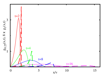
Figure 3: (Color online) Spatial dependence of the GF [Eq. (29)] for the model presented in Eq. (20) with continuous distribution of trap parameters corresponding to inverse-square-root singularity in the response function [see Eqs. (22) and (28))]. Dashed lines show the GF at $\rho_{1/2}=0.25$, while solid lines present the same GF at $\rho_{1/2}=1$ multiplied by the factor of $8$. We chose $t=2,4,8,12$ as indicated in the plot. Unlike in Fig. 2, due to abundance of traps with long release time, the GFs do not asymptotically converge toward a Gaussian form.

We also note that for large $t$ at any given $x$, Eq. (29) has a power-law tail $\propto t^{-3/2}$. This property is generic for continuous trap density distributions leading to small-$p$ power-law singularities in $\Sigma(p)$. For example, taking the density of the release rates as a power law in $B$,

$$\rho(B)={\sin(\pi s)\over\pi}{\rho_{s}\over B^{s}},$$ (30)

where $s$ is the corresponding exponent, $0<s<1$, we obtain $\Sigma(p)=\rho_{s}p^{-s}$, and the large-$t$ asymptotic of the GF at a fixed finite $x$ scales as

$$g(x,t)\propto t^{s-2}.$$ (31)

Such a power law is an essential feature of continuous distribution (30) of the detachments rates; it cannot be reproduced by a discrete set of rates $B_{i}$ which always produce an exponential tail.

IV Filtration under unfavorable conditions

IV.1 Multitrap model with saturation

The considered linearized filtration model presented by Eq. (20) can be used to analyze filtration of identical particles in small concentrations and over limited time interval as long as the trapped particles do not affect the filter performance. However, unless the model is used to simulate tracer particle dynamics in which no actual trapping occurs, it is unlikely that the model remains valid as the number of trapped particles grows.

Indeed, one expects that a trapped particle changes substantially the probability for subsequent particles to be trapped in its vicinity. Under favorable filtering conditions characterized by filter ripening OMelia-Ali-1978 ; Chiang-2004 , the probability of subsequent particle trapping increases with time as the number of trapped particles $n_{i}$ grows. On the other hand, under unfavorable filtering conditions, where the Debye screening length is large compared to the trap size $\ell$, for charged particles one expects trapping probabilities $A_{i}(n_{i})$ to decrease with $n_{i}$.

If repulsive force between particles is large, we can assume that only one particle is allowed to be captured in each trap. Subsequently, a single trap can be characterized by an attachment rate $A_{i}$ when it is empty and a detachment rate $B_{i}$ when it is occupied, and the mean-field trapping/release dynamics for a given group of trapping sites can be written as

$$\dot{n}_{i}=C\,A_{i}(1-n_{i})-B_{i}n_{i}.$$ (32)

Note that this equation is non-linear because it contains the product of $Cn_{i}$.

Previously, similar filtering dynamics was considered in a number of publications (see Refs. Bradford-2002 and Bradford-2003 and references therein). In the present work, we allow for a possibility of groups of traps differing by the rate parameters $A_{i}$ and $B_{i}$. The distribution of rate parameters can also be viewed as an analytical alternative of the computer-based models describing a network of pores of varying diameterRedner-2000 ; Kim-2006 ; shapiro-2007 .

Our mean-field transport model is completed by adding the kinetic equation for the motion of free particles with concentration $C$,

$$\dot{C}+vC^{\prime}+\sum_{i=1}^{m}N_{i}\dot{n}_{i}=0,$$ (33)

which has the same form as the linearized equations [Eq. (20)] considered in Sec. III.4.

We note that for shallow traps with large release rates $B_{i}$, the non-linearity inherent in Eq. (32) is not important for sufficiently small suspended particle concentrations $C$. Indeed, if $C$ is independent of time, the solution of Eq. (32) saturates at

$$n_{i}(C)={CA_{i}\over B_{i}+CA_{i}}.$$ (34)

For small free-particle concentration $C$, or for any $C$ and large enough $B_{i}$, the trap population is small compared to 1, and the non-linear term in Eq. (32) can be ignored.

Therefore, as discussed in relation with the linearized multitrap model [see Sec. IIIA and Eq. (20)], the effect of shallow traps is to introduce dispersivity of the arrival times of the particles on different trajectories. For this reason, we are free to drop the dispersivity term [cf. the CDE model, Eq. (1)], and use a simpler convection-only model (33) with several groups of traps with density $N_{i}$ per unit water volume, characterized by the relaxation parameters $A_{i}$ and $B_{i}$.

IV.2 General properties: Stable filtering front

The constructed non-linear equations [Eqs. (32) and (33)] describe complicated dynamics which is difficult to understand in general. Here, we introduce the front velocity, a parameter that characterizes the speed of deterioration of the filtering capacity.

Consider a semi-infinite filter, with the filtering medium initially clean, and the concentration $C(0,t)=C_{A}$ of suspended particles at the inlet constant. After some time, the concentration of deposited particles near the inlet reaches the dynamical equilibrium $n_{i}(C_{A})$ [Eq. (34)] and, on average, the particles will no longer be deposited there. At a given inlet concentration, the filtering medium near the inlet is saturated with deposited particles. On the other hand, sufficiently far from the inlet, the filter is still clean. On general grounds, there should be some crossover between these two regions.

The size of the saturated region grows with time [see Fig. 4]. The corresponding front velocity $v_{A}\equiv v(C_{A})$ can be easily calculated from the particle balance equation,

$$v_{A}C_{A}+v_{A}\sum_{i}N_{i}n_{i}(C_{A})=vC_{A}.$$ (35)

This equation balances the number of additional particles needed to increase the saturated region by $\delta x=v_{A}\delta t$ on the left, with the number of particles brought from the inlet on the right [see Fig. 4]. The same equation can also be derived if we set $C=C(x-v_{A}t)$, $n_{i}=n_{i}(x-v_{A}t)$ and integrate Eq. (33) over the entire crossover region. The trapped particle density saturates as given by Eq. (34), and the resulting front velocity is

$$v(C_{A})={v\over\displaystyle 1+\sum_{i}{N_{i}A_{i}\over A_{i}C_{A}+B_{i}}}.$$ (36)

This is a monotonously increasing function of $C_{A}$: larger inlet concentration $C_{A}$ leads to higher front velocity, which implies that the filtering front is stable with respect to perturbations. Indeed, in Appendix we show that the velocity $v_{AB}$ of a secondary filtering front with the inlet concentration $C_{B}>C_{A}$ (see Fig. 5), moving on the background of equilibrium concentration of free particles $C_{A}$, is higher than $v_{A}$, i.e., $v_{AB}>v_{A}$. Thus, if for some reason the original filtering front is split into two parts, moving with the velocities $v_{A}$ and $v_{AB}$, the secondary front will eventually catch up, restoring the overall front shape.

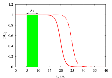
Figure 4: Solid line shows the free particle concentration near a filtering front. Dashed line shows the front shifted by $\Delta x$; the additional free and trapped particles in the shaded region are brought from the inlet [see Eq. (35)]. See Eq. (52) for exact front shape.

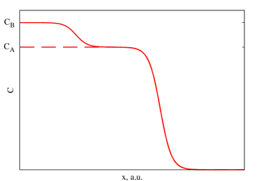
Figure 5: Free particle concentration $C(x,t)$ with two filtering fronts. The initial front moves on the background of clean filter and leaves behind the equilibrium filtering medium with $C=C_{A}$. The secondary front with higher inlet concentration $C_{B}$ is moving on partially saturated medium. With nonlinearity as in Eq. (32), the secondary front is always faster, $v_{AB}>v_{A}$; the two fronts will eventually coalesce into a single front.

We emphasize that the existence of the stable filtering front is in sharp contrast with the linearized filtering problem [see Eq. (20)], where the propagation velocity $v_{0}$ [Eq. (25)] is independent of the inlet concentration, and any structure is eventually washed out dispersively (the width of long-time GF does not saturate with time). Also, in the case of the filter ripening, the nonlinear term in Eq. (32) will be negative and thus would prohibit the filtering front solutions due to the fact that the secondary fronts move slower, $v_{AB}<v_{A}$. The non-linear problem with saturation is thus somewhat analogous to Korteweg-de Vries solitons where the dispersion and nonlinearity compete to stabilize the profilekdv ; drazin-book .

IV.3 Exactly solvable case

IV.3.1 General solution

Compared to the linear case presented in Sec. III, the physics behind the non-linear equations [Eqs. (32) and (33)] is much more complicated. However, the structure of these equations immediately indicates that non-linearity reduces filtering capacity because trapping sites could saturate in this model [see Eq. (34)]. While the relevant equations can also be solved numerically, a thorough understanding of the filtering system, especially with large or infinite number of traps, is difficult to achieve.

To gain some insight about the role of the different parameters in the filtering process, we specifically focus on the non-linear models presented by Eqs. (32) and (33) which can be rendered into a linear set of equations, very similar to the linear multitrap model [Eq. (20)]. To this end, we consider the case where all trapping sites have the same trapping cross sections, that is, all $A_{i}=A$ in Eq. (32). If we introduce the time integral

$$u(x,t)\equiv\int_{0}^{t}C(x,t^{\prime})dt^{\prime},$$ (37)

then Eq. (32) after a multiplication by $\exp Au$ can be written as

$${\partial_{t}}\left(n_{i}e^{Au}\right)+B_{i}\left(n_{i}e^{Au}\right)={\partial_{t}}\left(e^{Au}\right).$$ (38)

Clearly, these are a set of linear equations,

$$\dot{a}_{i}+B_{i}a_{i}=\dot{w},$$ (39)

with the following variables

$$w\equiv w(x,t)=e^{Au},\quad a_{i}\equiv a_{i}(x,t)=n_{i}\,w.$$ (40)

Note that Eq. (33) can also be written as a set of linear equations in terms of these variables. If we integrate Eq. (33) over time, we find

$$\dot{u}+vu^{\prime}+\sum_{i=1}^{m}N_{i}n_{i}=0,$$ (41)

where we assumed initially clean filter, $C(x,0)=n_{i}(x,0)=0$. Considering that $\dot{w}=A\dot{u}\,w$ and $w^{\prime}=Au^{\prime}\,w$, we obtain

$$\dot{w}+vw^{\prime}+A\,\sum_{i=1}^{m}N_{i}a_{i}=0.$$ (42)

The main difference of the linear Eqs. (39) and (42) from Eqs. (20) is in their initial and boundary conditions,

$$w(x,0) = 1,\quad a_{i}(x,0)=0,$$ (43)

$$w(0,t) = e^{Au_{0}(t)},\quad u_{0}(t)\equiv\int_{0}^{t}dt^{\prime}\,C(0,t^{\prime}).$$ (44)

Note that with the time-independent concentration of the particles in suspension at the inlet, i.e., $C(0,t)=C_{0}$, boundary condition (44) gives a growing exponent,

$$w_{0}(t)\equiv w(0,t)=e^{AC_{0}t}.$$ (45)

The derived equations can be solved with the use of the Laplace transformation. Denoting $\tilde{w}\equiv\tilde{w}(x,p)=\mathcal{L}_{p}\{w(t)\}$ and eliminating the Laplace-transformed trap populations $\tilde{n}_{i}(x,p)\equiv\mathcal{L}_{p}\{n_{i}(x,t)\}$, we obtain

$$(p\tilde{w}-1)\left[1+\Sigma(p)\right]+v\tilde{w}^{\prime}=0,\quad\Sigma(p)\equiv A\sum_{i}{N_{i}\over p+B_{i}}.$$ (46)

The response function $\Sigma(p)$ is identical to that in Eq. (22), and for the case of continuous trap distribution we can also introduce the effective density of traps, $\rho(B)\equiv A\sum_{i}N_{i}\delta(B-B_{i})$. The solution of Eq. (46) and the Laplace-transformed boundary condition [Eq. (44)] becomes

$$\tilde{w}={1\over p}+\left[\tilde{w}_{0}(p)-{1\over p}\right]e^{-[1+\Sigma(p)]px/v},$$ (47)

where $\tilde{w}(0,p)=\tilde{w}_{0}(p)$. Employing the same notation as in Eq. (21), the real-time solution of Eqs. (39) and (42) with the boundary conditions [Eqs. (43) and (44)] can be written in quadratures,

$$w(x,t)=1+\int_{0}^{t}dt^{\prime}\,\left[w_{0}(t-t^{\prime})-1\right]\,g(x,t^{\prime}).$$ (48)

The time-dependent concentration can be restored from here with the help of logarithmic derivative,

$$C(x,t)={1\over A}{\partial\,\ln w(x,t)\over\partial t}.$$ (49)

IV.3.2 Structure of the filtering front

In the special case $C(0,t)=C_{0}={\rm const}$, the integrated concentration [Eq. (37)] is linear in time at the inlet, $u_{0}(t)=C_{0}t$, and $w(0,t)$ grows exponentially [see Eq. (45)]. This exponent determines the main contribution to the integral in Eq. (48) for large $t$ and $x$. Indeed, in this case we can rewrite Eq. (48) exactly as $w(x,t)=1+J(C_{0})-J(0)$, where

$$J(C_{0})\equiv e^{AC_{0}t}\int_{0}^{t}dt^{\prime}\,e^{-AC_{0}t^{\prime}}g(x,t^{\prime}).$$ (50)

Note that $J(0)$ is proportional to the solution of the linearized equations [Eq. (20)] with time-independent inlet concentration $C(0,t)=\rm const$ [see Eq. (6)]. The corresponding front is moving with the velocity $v_{0}$ [Eq. (25)] and is widening over time [Eqs. (26) and (27)]. Thus, for $x/v_{0}-t$ positive and sufficiently large, this contribution to $w(x,t)$ is small and can be ignored. In the opposite limit of large negative $x/v_{0}-t$, $J(0)=1$, which exactly cancels the first term in Eq. (48).

On the other hand, the term $J(C_{0})$ grows exponentially large with time. At large enough $t$, the integration limit can be extended to infinity, and the integration in Eq. (50) becomes a Laplace transformation, thus

$$w(x,t) \approx 1+e^{AC_{0}t}\int_{0}^{\infty}dt^{\prime}\,e^{-AC_{0}t^{\prime}}g(x,t^{\prime})$$ (51)

$$= 1+e^{p_{0}t}\,e^{-[1+\Sigma(p_{0})]p_{0}x/v},\quad p_{0}\equiv AC_{0}.\qquad$$

This results in the following free-particle concentration [see Eq. (49)],

$$C(x,t)={C_{0}\over e^{[x/v(C_{0})-t]AC_{0}}+1},$$ (52)

and the occupation of the $i$th trap [Eqs. (39) and (40)],

$$n_{i}(x,t)={A\over B_{i}+AC_{0}}C(x,t),$$ (53)

with the front velocity

$$v(C_{0})\equiv{v\over 1+\Sigma(AC_{0})}.$$ (54)

Note that this coincides exactly with the general case presented in Eq. (36) if we set all $A_{i}=A$.

IV.3.3 Filtering front formation

The approximation in Eq. (51) is valid in the vicinity of the front, $|x/v(C_{0})-t|\lesssim(AC_{0})^{-1}$, as long as $x/v_{0}-t$ is positive and large. Since $v(C_{0})>v_{0}=v(0)$, this implies

$$x\left[{1\over v_{0}}-{1\over v(C_{0})}\right]\gg{1\over AC_{0}},$$ (55)

which provides an estimate of the distance from the outlet where the front structure [Eqs. (52) and (53)] is formed. The exactness of the obtained asymptotic front structure can be verified directly by substituting the obtained profiles in Eqs. (32) and (33).

The exact expressions in Eqs. (48) and (49) for the free-particle concentration can be integrated completely in some special cases. Here we list two such results and demonstrate the presence of striking similarities in the profiles $C(x,t)$ between different models, despite their very different rate distributions. Furthermore, we show that the corresponding exact solutions [Eq. (49)] converge rapidly toward the general filtering front [Eq. (52)].

Single-trap model with straining. In Sec. III.2, we found the explicit expression [Eq. (14)] for the GF in the case of the linear model for two types of trapping sites with rates $A_{1}$ and $B_{1}$ and permanent sites with the capture rate $A_{0}$. The resulting GF (with $A_{1}=A_{0}=A$ and $B_{1}=B$) can be used in Eq. (48) to construct the solution for the corresponding model with saturation,

$$\dot{C}+vC^{\prime}+N_{0}\dot{n}_{0}+N_{1}\dot{n}_{1}=0,$$ (56)

$$\dot{n}_{0}=AC(1-n_{0}),\quad\dot{n}_{1}=AC(1-n_{1})-B_{1}n_{1}.\quad$$ (57)

Let us consider the special case of the inlet concentration, $C(0,t)=C_{0}\,\theta(T-t)\,\theta(t)$, constant over the interval $0<t<T$, and zero afterwards. The function $w_{0}(t)$ [see Eq. (44)] is, then

$$w_{0}(t)=\exp[AC_{0}\min(t,T)],$$ (58)

and the integration in Eq. (48) gives

$$w=1+e^{-\beta\xi}\left[W(t)-e^{AC_{0}T}W(t-T)\right],$$ (59)

$$W(t)\equiv\theta(t-\xi)\Bigl{\{}\left[e^{AC_{0}(t-\xi)}-1\right]$$ (60)

$$\!\!\!+\int^{t}_{\xi}\!\!d\tau\,e^{-B_{1}(\tau-\xi)}\left[e^{AC_{0}(t-\tau)}-1\right]\frac{d}{d\tau}I_{0}(\zeta_{\tau})\Bigr{\}},\qquad\;$$

where $\xi\equiv x/v$ and $\zeta_{\tau}$ is given in Eq. (15). The concentration of free particles, $C(x,t)$, can be now obtained through Eq. (49). The step function $\theta(t-{x}/{v})$ included in $w$ indicates that it takes at least $t=x/v$ for a particle to travel a distance $x$.

Figure 6 illustrates $C(x,t)$ as a function of distance, $x$, at a set of discrete values of time $t=1$, $2$, …,$16$. The model parameters as indicated in the caption were obtained by fitting the response function $\Sigma(p)=AN_{0}/p+AN_{1}/(p+B_{1})$ at the interval $0.5<p<5.0$ to that of the model with the continuous trap distribution (see Fig. 7). The solid lines show the curves for $t\leq T$, while the dashed lines correspond to $t>T$; they have a drop in the concentration near the origin consistent with the boundary condition at the inlet. The exact profiles show excellent convergence toward the corresponding front profiles computed using Eq. (52) (symbols).

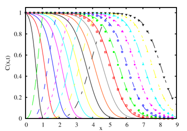
Figure 6: (Color online) Formation of the filtering front for the single-trap filtering model with straining [Eq. (56)]. Lines show the free-particle concentration $C(x,t)$ extracted from Eq. (56) with $T=10$, $A=v=C_{0}=1$, $N_{0}=0.388$, $N_{1}=3.60$, and $B_{1}=4.97$, for $t=1$, $2$, …,$16$. Symbols show the front solution [Eq. (52)] for $t\geq 10$ with the front velocity [Eq. (54)].

Model with square-root singularity. Let us now consider the non-linear model, [Eqs. (33) and (32)] with the inverse-square-root continuous trap distribution, producing the response function given in Eq. (28). The model is exactly solvable if we set all $A_{i}=A$, while allowing the trap densities $N_{i}$ vary with $B$ appropriately.

The solution for the auxiliary function $w$ corresponding to the inlet concentration $C(0,t)$ constant on an interval of duration $T$ is obtained by combining Eqs. (48) and (58), with the relevant GF [Eq. (29)]. The resulting $x$-dependent curves $C(x,t)$ at a set of discrete time values are shown in Fig. (7), along with the corresponding asymptotic front profiles (symbols), for a parameter set as indicated in the caption. The solid lines show the curves for $t\leq T$. The dashed lines are for $t>T$; they display a drop of the concentration near the origin consistent with the boundary condition at the inlet. Again, the time-dependent profiles show gradual convergence toward front solution (52).

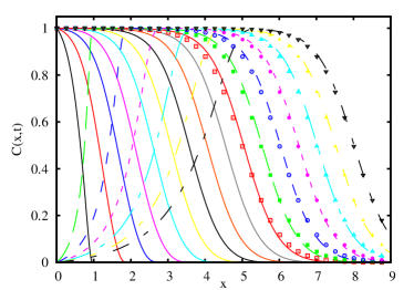
Figure 7: (Color online) As in Fig. 6 but for filtering model (33), Eq. (32) with continuous inverse-square-root trap distribution [Eq. (28)]. Parameters are $A=v=C_{0}=\rho_{1/2}=1$, $T=10$. Symbols show the front solution [Eq. (52)] for $t\geq 10$ with front velocity (54). The raising parts of the curves are almost identical with those in Fig. 6, while there are some quantitative differences in the tails, consistent with the exponential vs power-law long-time asymptotics of the corresponding solutions.

Note that the profiles in Figs. 6 and 7 are very similar even though the corresponding trap distributions differ dramatically. This illustrates that parameter fitting from a limited set of breakthrough curves is a problem ill-defined mathematically. The complexity and ambiguity of the problem grow with increasing number of traps. In Sec. V we suggest an alternative computationally simple procedure for parameter fitting using the data from several breakthrough curves differing by the input concentrations.

V Experimental implications

The suggested class of mean-field models is characterized by a large number of parameters. In the discrete case, these are the trap rate constants $A_{i}$, $B_{i}$ and the corresponding concentrations $N_{i}$ along with the flow velocity $v$. In the continuous case, the filtering medium is characterized by the response function $\Sigma(p)$ [see Eq. (22)]. In our experience, two or three sets of traps are usually sufficient to produce an excellent fit for a typical experimental breakthrough curve (not shown). This is not surprising, given the number of adjustable parameters. On the other hand, from Eq. (54) it is also clear that the obtained parameters would likely prove inadequate if we change the inlet concentration. The long-time asymptotic form of the effluent during the washout stage would also likely be off.

One alternative to a direct non-linear fitting is to use our result given in Eq. (54) [or Eq. (36)] for the filtering front velocity as a function of the inlet concentration, $C_{0}$. With a relatively mild assumption that all trapping rates coincide, $A_{i}=A$, one obtains the entire shape of the filtering front [Eq. (52)]. Thus, fitting the front profiles at different inlet concentrations $C_{0}$ to determine the parameter $A$ and the front velocity $v(C_{0})$ can be used to directly measure the response function $\Sigma(p)$.

The suggested experimental procedure can be summarized as follows. (i) One should use as long filtering columns as practically possible in order to achieve the front formation for a wider range of inlet concentrations. (ii) A set of breakthrough curves $C(L,t)$ for several concentrations $C_{0}$ at the inlet should be taken. (iii) For each curve, the front formation and the applicability of the simplified model with all $A_{i}=A$ should be verified by fitting with the front profile [Eq. (52)]. Given the column length, each fit would result in the front velocity $v(C_{0})$, as well as the inverse front width $p=AC_{0}$. (iv) The resulting data points should be used to recover the functional form of $\Sigma(p)$ and the solution for the full model.

It is important to emphasize that the applicability of the model can be controlled at essentially every step. First, the time-dependence of each curve should fit well with Eq. (52). Second, the values of the trapping rate $A$ obtained from different curves should be close. Third, the computed washout curves should be compared with the experimentally obtained breakthrough curves. The obtained parameters, especially the details of $\Sigma(p)$ for small $p$, can be further verified by repeating the experiments on a shorter filtering column with the same medium.

VI Conclusions

In this paper, we presented a mean-field model to investigate the transport of colloids in porous media. The model corresponds to the filtration under unfavorable conditions, where trapped particles tend to reduce the filtering capacity, and can also be released back to the flow. The situation should be contrasted with favorable filtering conditions characterized by filter ripening. These two different regimes can be achieved, e.g., by changing $p$H of the media if the colloids are charged. The unfavorable filtering conditions are typical for filtering encountered in natural environment, e.g., ground water with biologically active colloids such as viruses or bacteria.

The advantages of the model are twofold. It not only fixes some technical problems inherent in the mean-field models based on the CDE but also admits analytical solutions with many groups of traps or even with a continuous distribution of detachment rates. It is the existence of such analytical solutions that allowed us to formulate a well-defined procedure for fitting the coefficients. Ultimately, this improves predictive capability and accuracy of the model.

The need for the attachment and detachment rate distributions under unfavorable filtering conditions has already been recognized in the fieldBradford-2002 ; Bradford-2003 ; Yoon-2006 . Previously it has been implemented in computer-based models in terms of $ad$ $hoc$ distributions of the pore radiiRedner-2000 ; Kim-2006 ; shapiro-2007 . Such models could result in good fits to the experimental breakthrough curves. However, we showed in Sec.V that the relevant experimental curves are often insensitive to the details of the trap parameter distributions, especially on the early stages of filtering.

On the other hand, our analysis of the filtering front reveals that the front velocity as a function of the inlet colloid concentration, $v(C_{0})$ [Eq. (36)], is primarily determined by the distribution of the attachment and detachment rates characterizing the filtering medium. We, indeed, suggest that the filtering front velocity is one of the most important characteristics of the deep-bed filtration as it is directly related to the loss of filtering capacity.

We have developed a detailed protocol to calculate the model parameters based on the experimentally determined front velocity, $v(C_{0})$. We emphasize that the most notable feature of the model is its ability to distinguish between permanent traps (straining) and the traps with small but finite detachment rate. It is the latter traps that determine the long-time asymptotics of the washout curves.

The suggested model is applicable to a wide range of problems in which macromolecules, stable emulsion drops, or pathogenic micro-organisms such as bacteria and viruses are transported in flow through a porous medium. While the model is purely phenomenological in nature, the mapping of the parameters with the experimental data as a function of flow velocity and colloid size will shed light on the nature of trapping for particular colloids. The model can also be extended to account for variations in attachment and detachment rates for various colloids as needed to explain the steep deposition profiles near the inlet of filtersli-2004 .

Appendix A Velocity of an intermediate front.

Here we derive an inequality for the velocity $v_{AB}$ of an intermediate front interpolating between free-particle concentrations $C_{A}$ and $C_{B}$ [Fig. 5].

We first write the expressions for the filtering front velocities in clean filter, with the inlet concentrations $C_{A}$ and $C_{B}>C_{A}$ [cf. Eq. (35)],

$$\left({v\over v_{A}}-1\right)C_{A} = \sum_{i}N_{i}n_{i}(C_{A}),$$

$$\left({v\over v_{B}}-1\right)C_{B} = \sum_{i}N_{i}n_{i}(C_{B}).$$

The velocity $v_{AB}$ of the filtering front interpolating between $C_{A}$ and $C_{B}$ [Fig. 5] is given by

$$\left({v\over v_{AB}}-1\right)(C_{B}-C_{A})=\sum_{i}N_{i}[n_{i}(C_{B})-n_{i}(C_{A})].$$ (61)

Combining these equations, we obtain

$${C_{B}\over v_{B}}-{C_{A}\over v_{A}}={C_{B}-C_{A}\over v_{AB}}.$$ (62)

From here we conclude that the left-hand side (lhs) of Eq. (62) is positive. Solving for $v_{AB}$ and expressing the difference $v_{AB}-v_{A}$, we have

$$v_{AB}-v_{A}={C_{B}(v_{B}-v_{A})\over\displaystyle\left({C_{B}\over v_{B}}-{C_{A}\over v_{A}}\right)v_{B}}.$$ (63)

For the model with saturation [Eq. (32)], we saw that $v_{B}>v_{A}$, thus $v_{AB}>v_{A}$.

References

- (1) A. O. Imdakm and M. Sahimi, Phys. Rev. A 36, 5304 (1987).
- (2) L. Bloomfield, Sci. Am. 281, 152 (1999).
- (3) L. Luhrmann, U. Noseck, and C. Tix, Water Resour. Res. 34, 421 (1998).
- (4) R. W. Harvey and S. P. Garabedian, 25, 178 (1991).
- (5) J. P. Herzig, D. M. Leclerc, and P. le Goff, Ind. Eng. Chem. 62, 8 (1970).
- (6) C. Tien and A. C. Payatakes, AIChE J. (1979).
- (7) H.-W. Chiang and C. Tien, AIChE J. 31, 1360 (1985).
- (8) S. Vigneswaran and C. J. Song, Water, Air, Soil Pollut. 29, 155 (1986).
- (9) S. Vigneswaran and R. K. Tulachan, Water Res. 22, 1093 (1988).
- (10) C. Ghidaglia. E. Guazzelli and L. Oger, J. Phys. D 24, 2111 (1991).
- (11) J. E. Tobiason and B. Vigneswaran, Water Res. 28, 335 (1994).
- (12) J. Lee and J. Koplik, Phys. Rev. E 54, 4011 (1996).
- (13) S. Vigneswaran and J. S. Chang, Water Res. 23, 1413 (1989).
- (14) V. Jegatheesan and S. Vigneswaran, Crit. Rev. Environ. Sci. Technol. 35, 515 (2005).
- (15) O. Albinger, B. K. Biesemeyer, R. G. Arnold, and B. E. Logan, FEMS Microbiol. Lett. 124, 321 (1994).
- (16) J. C. Baygents et al., Environ. Sci. Technol. 32, 1596 (1998).
- (17) S. F. Simoni, H. Harms, T. N. P. Bosma, and A. J. B. Zehnder, Environ. Sci. Technol. 32, 2100 (1998).
- (18) C. H. Bolster, A. L. Mills, G. M. Hornberger, and J. S. Herman, Water Resour. Res. 35, 1797 (1999).
- (19) C. H. Bolster, A. L. Mills, G. Hornberger, and J. Herman, Ground Water 38, 370 (2000).
- (20) J. A. Redman, S. B. Grant, T. M. Olson, and M. K. Estes, Environ. Sci. Technol. 35, 1798 (2001).
- (21) J. A. Redman, M. K. Estes, and S. B. Grant, Colloids Surf. A 191, 57 (2001).
- (22) N. Tufenkji, J. A. Redman, and M. Elimelech, Environ. Sci. Technol., 37, 616 (2003).
- (23) X. Li, T. D. Scheibe, and W. P. Johnson, Environ. Sci. Technol. 38, 5616 (2004).
- (24) S. A. Bradford, S. Yates, M. Bettahar, and J. Simunek, Water Resour. Res. 38, 1327 (2002).
- (25) S. A. Bradford, J. Simunek, M. Bettahar, M. T. van Genuchten, and S. R. Yates, Environ. Sci. Technol. 37, 2242 (2003).
- (26) J. S. Yoon, J. T. Germaine, and P. J. Culligan, Water Resour. Res. 42, W06417 (2006).
- (27) S. Redner and S. Datta, Phys. Rev. Lett. 84, 6018 (2000).
- (28) W. Hwang and S. Redner, Phys. Rev. E 63, 021508 (2001).
- (29) Y. S. Kim and A. J. Whittle, Transp. Porous Media 65, 309 (2006).
- (30) A. Shapiro, P. G. Bedrikovetsky, A. Santos, and O. Medvedev, Transp. Porous Media 67, 135 (2007).
- (31) T. D. Scheibe and B. D. Wood, Water Resour. Res. 39, 1080 (2003).
- (32) L. Lapidus and N. R. Amundson, J. Phys. Chem. 56, 984 (1952).
- (33) T. Jevremovic, Nuclear Principles in Engineering, (Springer, New York, 2005), Chap. 7, pp.297-396.
- (34) R. Haggerty and S. M. Gorelick, Water Resour. Res. 31, 2383 (1995).
- (35) Note that Eq. (14) can also be written as a time derivative, .
- (36) C. R. O’Melia and W. Ali, Prog. in Water Technol. 10, 167 (1978).
- (37) H.-W. Chiang and C. Tien, AIChE J. 31, 1349 (1984).
- (38) D. J. Korteweg and G. de Vries, Philos. Mag. 39, 422 (1895).
- (39) P. G. Drazin, Solitons, London Mathematical Society Lecture Note Series, Vol. 85 (Cambridge University Press, Cambridge, 1983).