$\Lambda$-doublet spectra of diatomic radicals and their dependence on fundamental constants

Abstract

$\Lambda$-doublet spectra of light diatomic radicals have high sensitivity to the possible variations of the fine structure constant $\alpha$ and electron-to-proton mass ratio $\beta$. For molecules OH and CH sensitivity is further enhanced because of the $J$-dependent decoupling of the electron spin from the molecular axis, where $J$ is total angular momentum of the molecule. When $\Lambda$-splitting has different signs in two limiting coupling cases $a$ and $b$, decoupling of the spin leads to the change of sign of the splitting and to the growth of the dimensionless sensitivity coefficients. For example, sensitivity coefficients for the $\Lambda$-doublet lines $J=\tfrac{9}{2}$ of the $\Pi_{1/2}$ state of OH molecule are on the order of $10^{3}$.

I Introduction

At present an intensive search is going on for the possible space and time variations of fundamental constants (FC). On a short time scale very tight bounds on such variations were obtained in laboratory experiments Rosenband et al. (2008); Shelkovnikov et al. (2008). On the other hand astrophysical observations provide information on the variation of FC on the timescale of the order of $10^{10}$ years. Here results of Ref. Murphy et al. (2003) indicate variation on the level of five sigma, $\Delta\alpha/\alpha=(-0.57\pm 0.11)\times 10^{-5}$. At the same time, Ref. Srianand et al. (2004) reports no variation, $\Delta\alpha/\alpha=(-0.06\pm 0.06)\times 10^{-5}$, and Ref. Levshakov et al. (2007) reports variation of the opposite sign, $\Delta\alpha/\alpha=(+0.54\pm 0.25)\times 10^{-5}$. An intermediate timescale $\sim 2\times 10^{9}$ years is tested by the Oklo phenomenon Shlyakhter (1976); Flambaum and Wiringa (2009).

Recently there was much attention in this context to the microwave spectra of molecules. Generally these spectra are sensitive to possible variations of the electron to proton mass ratio $\beta=m_{e}/m_{p}$. When fine and hyperfine structures are involved, they also become sensitive to variations of the fine structure constant $\alpha$ and nuclear $g$-factor $g_{\mathrm{nuc}}$. There were several proposals of microwave experiments with diatomic molecules. Rotational microwave spectra were used numerous times to study time variation of fundamental constants in astrophysics. However, all such lines have same dependence on FC, $\delta\omega_{\mathrm{rot}}/\omega_{\mathrm{rot}}=\delta\beta/\beta$, so one needs to use reference lines with different dependence on FC. In the microwave band there are several examples of such lines (see Table 1).

Table 1: Quantum numbers and frequencies of microwave lines used for astrophysical studies of possible variation of FC. For $\Lambda$ transitions of CH and OH molecules only one of the strongest hyperfine components is given. Ammonia inversion transition has rotational structure described by quantum numbers $J$ and $K$, where $K$ is projection of the angular momentum $\bm{J}$ on the molecular axis, and smaller hyperfine structure, described by the total angular momentum quantum number $F$ and intermediate quantum number $F_{1}$. Here we present one of the 18 hyperfine components of the inversion line $(J,K)=(1,1)$.

Atom/molecule	$\lambda$ (cm)	Quantum numbers	Frequency (MHz)	Ref.
H	$21$	$1s_{1/2},\,F=0-1$	$1420.405751767(1)$	Essen et al. (1971)
OH	$18$	$\Pi_{3/2},\,J=\tfrac{3}{2},F=2$	$1667.358996(4)$	Hudson et al. (2006)
CH	$9.0$	$\Pi_{1/2},\,J=\tfrac{1}{2},F=1$	$3335.481(1)$	McCarthy et al. (2006)
CH	$42$	$\Pi_{3/2},\,J=\tfrac{3}{2},F=2$	$701.677(10)$	Ziurys and Turner (1985)
CH	$4.1$	$\Pi_{1/2},\,J=\tfrac{3}{2},F=2$	$7348.419(1)$	McCarthy et al. (2006)
NH3	$1.2$	$(J,K)=(1,1);\,F,F_{1}=\tfrac{1}{2},1$	$23694.4591(1)$	Kukolich (1967)

First, the famous 21 cm hydrogen hyperfine line depends on all three FC, $\delta\omega_{\mathrm{hf}}/\omega_{\mathrm{hf}}=\delta{\cal F}/{\cal F}$, ${\cal F}=\alpha^{2}\beta g_{\mathrm{nuc}}$ (note that the 21 cm line of hydrogen was used to constrain variation of FC as early as 1956 Savedoff (1956)). Second, the 18 cm $\Lambda$-doublet line of OH molecule depends on $\alpha$ and $\beta$ as follows: $\delta\omega_{\mathrm{OH}}/\omega_{\mathrm{OH}}=\delta{\cal F}/{\cal F}$, ${\cal F}=\alpha^{-1.14}\beta^{2.57}$ Darling (2003); Chengalur and Kanekar (2003); Kanekar et al. (2004). Third, the 1.2 cm inversion line of ammonia depends only on $\beta$, $\delta\omega_{\mathrm{inv}}/\omega_{\mathrm{inv}}=4.46\,\delta\beta/\beta$ van Veldhoven et al. (2004); Flambaum and Kozlov (2007). Finally, the fine structure far infrared 158 $\mu$m line of C II is sensitive only to $\alpha$, $\delta\omega_{\mathrm{fs}}/\omega_{\mathrm{fs}}=2\delta\alpha/\alpha$. All these four reference lines were used in combination with some rotational lines to put strong limits on variation of FC Murphy et al. (2001); Kanekar et al. (2005); Flambaum and Kozlov (2007); Murphy et al. (2008); Levshakov et al. (2008a).

If the Hydrogen 21-cm line is used as a reference for 18-cm OH line, the combination of constants, which is constrained, has the form Kanekar et al. (2005):

$${\cal F}=\alpha^{3.14}\beta^{-1.57}g_{\mathrm{nuc}}\,.$$ (1)

The most tight limit on the variation of $\cal F$ was obtained from observations of the absorber at the redshift $z=0.765$ and the $z=0.685$ gravitational lens, Ref. Kanekar et al. (2005):

$$\delta{\cal F}/{\cal F}=\left(0.44\pm 0.36^{\mathrm{stat}}\pm 1.0^{\mathrm{syst}}\right)\times 10^{-5}\,.$$ (2)

For OH molecule at least two more $\Lambda$-doublet lines were detected from interstellar medium in addition to the lowest 18 cm line, which was used in Ref. Kanekar et al. (2005). Sensitivity coefficient for these lines were found in Ref. Kanekar and Chengalur (2004). They appeared to be rather different from those of the lowest $\Lambda$-doublet line. Therefore, it is possible to use different $\Lambda$-doublet lines of the OH molecule to place a limit on the variation of fundamental constants without using reference lines of other species. This can help to eliminate systematic effect from the different velocity distributions of different species in molecular clouds. Two lowest $\Lambda$-doublet lines of CH molecule (9 cm and 42 cm) were detected in the interstellar medium Rydbeck et al. (1974); Ziurys and Turner (1985). Recently Christian Henkel and Karl Menten suggested that these lines can be used for astrophysical search of the time-variation of fundamental constants Henkel and Menten (2008). There are also several other light molecules with $\Lambda$-doubling, where microwave spectra were observed in the interstellar medium. For example, first extragalactic microwave rotational spectra of NO were observed in Martín et al. (2003). Therefore, we decided to study sensitivities of the $\Lambda$-doublet lines to the variation of the fundamental constants in a more systematic way.

Astrophysical studies of variation of fundamental constants require accurate knowledge of the laboratory frequencies. In the microwave band it is not so rare that the accuracy of the astrophysical observations is higher than the accuracy of the respective laboratory measurements. Therefore, some of the recommended “laboratory” frequencies are actually recalculated from astrophysical spectra (see, for example, Ziurys and Turner (1985); Pagani et al. (2009)). This method is based on the assumption that different lines from the same distant object have the same redshifts. Thus, the redshift is first determined from one set of lines and then is used to find rest frame frequencies of the other set of observed lines. The logic in these works is opposite to the one used in the search of the variation of FC. In such a search one looks for the difference in the apparent redshifts of the lines from the same object and compare these differences to the sensitivities of respective lines to variation of the constants to get information on constant variation.

Recently the laboratory frequencies of all four hyperfine components of the 18 cm line of OH molecule were measured with a record precision $(<10^{-9})$ Lev et al. (2006); Hudson et al. (2006). Also, the frequencies of all three components of the 9 cm $\Lambda$-doublet line $J=\tfrac{1}{2}$ in CH molecule were recently remeasured in Ref. McCarthy et al. (2006) with the accuracy of 0.1 ppm, or better ($1\,\mathrm{ppm}=10^{-6}$). This opens possibility to study variation of fundamental constants at the level below 1 ppm. Such studies can supplement the limits on $\beta$-variation based on the observations of the ammonia inversion line Flambaum and Kozlov (2007); Murphy et al. (2008); Levshakov et al. (2008b); Henkel et al. (2009) because $\Lambda$-doublet lines are sensitive to variation of $\alpha$ and $\beta$, while ammonia line is sensitive only to $\beta$. Moreover, as we will show below, because of the decoupling of the electron spin from the molecular axis, the sensitivity coefficients here strongly depend on the rotational quantum numbers. Therefore, if more than one line is observed, it may be possible to obtain model independent limits on variation of both constants. Sensitivity to the third constant $g_{\mathrm{nuc}}$ is typically much weaker, except for some low frequency lines where hyperfine contribution to transition frequency becomes significant. If such lines are observed, it is possible to make full experiment and constrain variation of all three constants.

Additional motivation to the present work comes from rapid progress in laboratory experiments with cold and ultracold molecules. New laboratory techniques can make it possible to use molecular $\Lambda$-doublet lines for laboratory tests on variation of FC. The most recent developments in this field are summarized in the review Carr et al. (2009).

In this paper we estimate sensitivity coefficients of different $\Lambda$-doublet lines to variations of constants $\alpha$, $\beta$, and $g_{\mathrm{nuc}}$. The analysis is basically the same for all light molecules in the ${}^{2}\Pi_{1/2}$, or ${}^{2}\Pi_{3/2}$ states. We include several of them here, for which there is sufficient data in the databases of microwave molecular spectra Lovas et al. ; Chen et al. ; Müller et al. . We use this data to find parameters of the effective spin-rotational Hamiltonian and to calculate sensitivity coefficients.

II Sensitivity coefficients

We restrict ourselves to the case of the diatomic radicals in doublet states ${}^{2}\Pi_{1/2}$, or ${}^{2}\Pi_{3/2}$. Let us define dimensionless sensitivity coefficients to the variation of FC so that:

$$\frac{\delta\omega}{\omega}=K_{\alpha}\frac{\delta\alpha}{\alpha}+K_{\beta}\frac{\delta\beta}{\beta}+K_{g}\frac{\delta g_{\mathrm{nuc}}}{g_{\mathrm{nuc}}}\,.$$ (3)

Dimensionless sensitivity coefficients $K_{i}$ are most relevant in astrophysics, where lines are Doppler broadened, so $\Gamma\approx\Gamma_{D}=\omega\times\Delta v/c$, where $\Delta v$ is velocity variance and $c$ is the speed of light. The redshift of a given line is defined as $z_{i}=\omega_{\mathrm{lab},i}/\omega_{i}-1$. Frequency shift (3) leads to the change in the apparent redshifts of individual lines. The difference in the redshifts of two lines is given by:

$$\frac{z_{i}-z_{j}}{1+z}=-\Delta K_{\alpha}\frac{\delta\alpha}{\alpha}-\Delta K_{\beta}\frac{\delta\beta}{\beta}-\Delta K_{g}\frac{\delta g_{\mathrm{nuc}}}{g_{\mathrm{nuc}}}\,.$$ (4)

where $z$ is the average redshift of both lines and $\Delta K_{\alpha}=K_{\alpha,i}-K_{\alpha,j}$, etc. We can rewrite Eq. (4) in terms of the variation of a single parameter $\cal F$:

$$\frac{z_{i}-z_{j}}{1+z}=-\frac{\delta{\cal F}}{\cal F}\,,\quad{\cal F}\equiv\alpha^{\Delta K_{\alpha}}\beta^{\Delta K_{\beta}}g_{\mathrm{nuc}}^{\Delta K_{g}}\,.$$ (5)

The typical values of $\Delta v$ for the extragalactic spectra is on the order of few km/s. This determines the accuracy of the redshift measurements on the order of $\delta z=10^{-5}$ – $10^{-6}$, practically independent on the transition frequency. Therefore, the sensitivity of astrophysical spectra to variations of FC directly depend on $\Delta K_{i}$.

In optical range sensitivity coefficients are typically on the order of $10^{-2}$ – $10^{-3}$, while in microwave and far infrared frequency regions they are typically on the order of unity. In fact, as we will see below, in some special cases sensitivity coefficients can be much greater that unity. This makes observations in microwave and far infrared wavelength regions potentially more sensitive to variations of FC, as compared to observations in optical region. Because of the lower sensitivity, systematic effects in optics may be significantly larger (for the most recent discussion of the systematic effects see Griest et al. (2009) and references therein).

In Sec. II.1 we briefly recall the theory of $\Lambda$- and $\Omega$-doubling in the pure coupling cases $a$ and $b$ and find respective sensitivity coefficients. After that we will calculate sensitivity coefficients for particular molecules using simplified variant of effective Hamiltonian from Ref. Meerts and Dymanus (1972). This Hamiltonian accounts for decoupling phenomena and for the hyperfine structure of $\Lambda$-doublets. We fit free parameters of this Hamiltonian to match experimental frequencies. After that we use numerical differentiation to find sensitivity coefficients.

II.1 $\Lambda$-doubling and $\Omega$-doubling

Consider electronic state with nonzero projection $\Lambda$ of the orbital angular momentum on the molecular axis. The spin-orbit interaction couples electron spin $\bm{S}$ to the molecular axis, its projection being $\Sigma$. To a first approximation the spin-orbit interaction is reduced to the form $H_{so}=A\Lambda\Sigma$. Total electronic angular momentum $\bm{J}_{e}=\bm{L}+\bm{S}$ has projection $\Omega$ on the axis, $\Omega=\Lambda+\Sigma$. For a particular case of $\Lambda=1$ and $S=\tfrac{1}{2}$ we have two states $\Pi_{1/2}$ and $\Pi_{3/2}$ and the energy difference between them is: $E(\Pi_{3/2})-E(\Pi_{1/2})=A$.

Rotational energy of the molecule is described by the Hamiltonian:

$$H_{\mathrm{rot}} =B(\bm{J}-\bm{J}_{e})^{2}$$ (6a)

$$=B\bm{J}^{2}-2B(\bm{JJ}_{e})+B\bm{J}_{e}^{2}\,$$ (6b)

where $B$ is rotational constant and $\bm{J}$ is the total angular momentum of the molecule. The first term in expression (6b) describes conventional rotational spectrum. The last term is constant for a given electronic state and can be added to the electronic energy. The second term describes $\Omega$-doubling and is known as Coriolis interaction $H_{\mathrm{Cor}}$.

If we neglect Coriolis interaction, the eigenvectors of Hamiltonian (6) have definite projections $M$ and $\Omega$ of the molecular angular momentum $\bm{J}$ on the laboratory axis and on the molecular axis respectively. In this approximation the states $|J,M,\Lambda,\Sigma,\Omega\rangle$ and $|J,M,-\Lambda,-\Sigma,-\Omega\rangle$ are degenerate, $E_{J,\pm\Omega}=BJ(J+1)$. Coriolis interaction couples these states and removes degeneracy. New eigenstates are the states of definite parity $p=\pm 1$ Brown and Carrington (2003):

$$|J,M,\Omega,p\rangle =\left(|J,M,\Omega\rangle+p(-1)^{J-S}|J,M,-\Omega\rangle\right)/\sqrt{2}\,,$$ (7)

Operator $H_{\mathrm{Cor}}$ can only change quantum number $\Omega$ by one, so the coupling of states $|\Omega\rangle$ and $|-\Omega\rangle$ takes place in the $2\Omega$ order of the perturbation theory in $H_{\mathrm{Cor}}$.

$\Omega$-doubling for the state $\Pi_{1/2}$ happens already in the first order in Coriolis interaction, but has additional smallness from the spin-orbit mixing. Operator $H_{\mathrm{Cor}}$ can not directly mix degenerate states $|\Lambda=1,\Sigma=-\tfrac{1}{2},\Omega=\tfrac{1}{2}\rangle$ and $|\Lambda=-1,\Sigma=\tfrac{1}{2},\Omega=-\tfrac{1}{2}\rangle$ because it requires changing $\Lambda$ by two. Therefore, we need to consider spin-orbit mixing between $\Pi$ and $\Sigma$ states:

$$|\Omega=\tfrac{1}{2}\rangle =|\Lambda=1,\Sigma=-\tfrac{1}{2},\Omega=\tfrac{1}{2}\rangle$$

$$+\zeta|\Lambda=0,\Sigma=\tfrac{1}{2},\Omega=\tfrac{1}{2}\rangle,$$ (8)

where

$$\zeta\sim A/(E_{\Pi}-E_{\Sigma}),$$ (9)

and then

$$\langle\Omega=\tfrac{1}{2}|H_{\mathrm{Cor}}|\Omega=-\tfrac{1}{2}\rangle=2\zeta B(J+\tfrac{1}{2})\langle\Lambda=1|L_{x}|\Lambda=0\rangle.$$ (10)

Note that $\zeta$ depends on the non-diagonal matrix element of spin-orbit interaction and Eq. (9) is only an order of magnitude estimate. It is important, though, that non-diagonal and diagonal matrix elements have similar dependence on FC. We conclude that $\Omega$-splitting for the $\Pi_{1/2}$ level must scale as $ABJ/(E_{\Pi}-E_{\Sigma})$.

The $\Omega$-doubling for $\Pi_{3/2}$ state takes place in the third order in Coriolis interaction. Here $H_{\mathrm{Cor}}$ has to mix first states $\Pi_{3/2}$ with $\Pi_{1/2}$ and $\Pi_{-3/2}$ with $\Pi_{-1/2}$ before matrix element (10) can be used. Therefore, the splitting scales as $B^{3}J^{3}/[A(E_{\Pi}-E_{\Sigma})]$.

The above consideration corresponds to the coupling case $a$, when $|A|\gg B$. In the opposite limit the states $\Pi_{1/2}$ and $\Pi_{3/2}$ are strongly mixed by the Coriolis interaction and spin $\bm{S}$ decouples from the molecular axis (coupling case $b$). As a result, the quantum numbers $\Sigma$ and $\Omega$ are not defined and we only have one quantum number $\Lambda=\pm 1$. Now $\Lambda$-splitting takes place in the second order in Coriolis interaction via intermediate $\Sigma$ state. The scaling here is obviously of the form $B^{2}J^{2}/(E_{\Pi}-E_{\Sigma})$. Note that in contrast to the previous case $|A|\gg B$, the splitting here is independent on $A$.

We can now use found scalings of the $\Lambda$- and $\Omega$-doublings to determine sensitivity coefficients (3). For this we only need to know how parameters $A$ and $B$ depend on $\alpha$ and $\beta$. In atomic units these parameters obviously scale as: $A\propto\alpha^{2}$ and $B\propto\beta$. We conclude, that for the case $a$ the $\Omega$-doubling spectrum has following sensitivity coefficients:

$$\mathrm{State\,}^{2}\Pi_{1/2}:\quad K_{\alpha}=\phantom{-}2\,,\quad K_{\beta}=1\,,$$ (11a)

$$\mathrm{State\,}^{2}\Pi_{3/2}:\quad K_{\alpha}=-2\,,\quad K_{\beta}=3\,.$$ (11b)

For the case $$b \bm{S} \Lambda$$, when is completely decoupled from the axis, the -doubling spectrum has following sensitivity coefficients:

$$\mathrm{State\,\,}\Pi:\quad K_{\alpha}=0\,,\quad K_{\beta}=2\,.$$ (11c)

When constant $A$ is slightly larger than $B$, the spin $\bm{S}$ is coupled to the axis only for lower rotational levels. As rotational energy grows with $J$ and becomes larger than the splitting between states $\Pi_{1/2}$ and $\Pi_{3/2}$, the spin decouples from the axis. Consequently, the $\Omega$-doubling is transformed into $\Lambda$-doubling. Equations (11) show that this can cause significant changes in sensitivity coefficients. The spin-orbit constant $A$ can be either positive (CH molecule), or negative (OH). The sign of the $\Omega$-doubling depends on the sign of $A$, while $\Lambda$-doubling does not depend on $A$ at all. Therefore, decoupling of the spin can change the sign of the splitting. In Sec. II.2 we will see that this can lead to the dramatic enhancement of the sensitivity to the variation of FC.

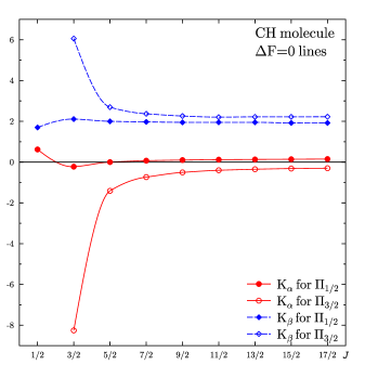
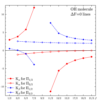
Figure 1: Sensitivity coefficients $K_{\alpha}$ and $K_{\beta}$ for $\Lambda$-doublet lines with $\Delta F=0$ in CH and OH molecules. The difference between lines with $F=J+\tfrac{1}{2}$ and $F=J-\tfrac{1}{2}$ is too small to be seen. For the state $\Pi_{3/2}$ of OH molecule the values for $J=\tfrac{9}{2}$ are too large to be shown on the plot. They are listed in Table 2.

II.2 Intermediate coupling

$\Lambda$-doubling for the intermediate coupling was studied in detail in many papers, including Meerts and Dymanus (1972); Brown et al. (1979); Brown and Merer (1979) (see also the book Brown and Carrington (2003)). Here we use effective Hamiltonian $H_{\mathrm{eff}}$ from Ref. Meerts and Dymanus (1972) in the subspace of the levels $\Pi_{1/2}^{\pm}$ and $\Pi_{3/2}^{\pm}$, where upper sign corresponds to parity $p$ in Eq. (7). Operator $H_{\mathrm{eff}}$ includes spin-rotational and hyperfine parts:

$$H_{\mathrm{eff}} =H_{\mathrm{sr}}+H_{\mathrm{hf}}\,.$$ (12)

Neglecting third order terms in Coriolis and spin-orbit interactions, we get the following simplified form of spin-rotational part:

$$\langle\Pi_{1/2}^{\pm}|H_{\mathrm{sr}}|\Pi_{1/2}^{\pm}\rangle =-\tfrac{1}{2}A+B(J+\tfrac{1}{2})^{2}$$

$$\pm(S_{1}+S_{2})(2J+1)\,,$$ (13a)

$$\langle\Pi_{3/2}^{\pm}|H_{\mathrm{sr}}|\Pi_{3/2}^{\pm}\rangle =+\tfrac{1}{2}A+B(J+\tfrac{1}{2})^{2}-2B\,,$$ (13b)

$$\langle\Pi_{3/2}^{\pm}|H_{\mathrm{sr}}|\Pi_{1/2}^{\pm}\rangle =\left[B\pm S_{2}(J+\tfrac{1}{2})\right]$$

$$\times\sqrt{(J-\tfrac{1}{2})(J+\tfrac{3}{2})}\,,$$ (13c)

Here in addition to parameters $A$ and $B$ we have two parameters, which appear in the second order of perturbation theory via intermediate state(s) $\Sigma_{1/2}$. Parameter $S_{1}$ corresponds to the cross term of the perturbation theory in spin-orbit and Coriolis interactions, while parameter $S_{2}$ is quadratic in Coriolis interaction. Because of this $S_{1}$ scales as $\alpha^{2}\beta$ and $S_{2}$ scales as $\beta^{2}$. The third order parameters neglected in (13) consist of several terms each with different dependencies on parameters $\alpha$ and $\beta$ Meerts and Dymanus (1972). For this reason we can not use them to study sensitivity coefficients. Fortunately, all third order terms are very small for the molecules considered here. They account only for the fine tuning of the spectrum and do not noticeably affect sensitivity coefficients for transitions with moderate quantum numbers $J$. It is easy to see that Hamiltonian $H_{\mathrm{sr}}$ describes limiting cases $|A|\gg B$ and $|A|\ll B$ considered in Sec. II.1.

The hyperfine part of effective Hamiltonian is defined in the lowest order of perturbation theory and has the form:

$$\langle\Pi_{1/2}^{\pm}|H_{\mathrm{hf}}|\Pi_{1/2}^{\pm}\rangle =C_{F}\left[2a-b-c\pm(2J+1)d\right],$$ (14a)

$$\langle\Pi_{3/2}^{\pm}|H_{\mathrm{hf}}|\Pi_{3/2}^{\pm}\rangle =3C_{F}\left[2a+b+c\right],$$ (14b)

$$\langle\Pi_{3/2}^{\pm}|H_{\mathrm{hf}}|\Pi_{1/2}^{\pm}\rangle =-C_{F}\sqrt{(2J-1)(2J+3)}\,b\,,$$ (14c)

$$C_{F} \equiv\frac{F(F+1)-J(J+1)-I(I+1)}{8J(J+1)}\,.$$

Here we assume that only one nucleus has spin and include only magnetic dipole hyperfine interaction. In this approximation all four parameters of $H_{\mathrm{hf}}$ scale as $\alpha^{2}\beta g_{\mathrm{nuc}}$.

Effective Hamiltonian described by Eqs. (13,14) has 8 parameters. We use NIST values Lovas et al. for the fine structure splitting $A$, rotational constant $B$, and magnetic hyperfine constants $a$, $b$, $c$, $d$. Remaining two parameters $S_{1}$ and $S_{2}$ are found by minimizing rms deviation between theoretical and experimental $\Lambda$-doubling spectra.

In order to find sensitivity coefficients $K_{\alpha}$ we calculate transition frequency for two values of $\alpha=\alpha_{0}\pm\delta$ near its physical value $\alpha_{0}=1/137.035999679(94)$ and similarly for $K_{\beta}$ and $K_{g}$. We use scaling rules discussed above to recalculate parameters of the effective Hamiltonian for different values of FC. Then we use numerical differentiation to find respective sensitivity coefficient.

We check the accuracy of our approach by adding three most important third order parameters from Ref. Meerts and Dymanus (1972) to Hamiltonian (13) and including them in fitting procedure. That leads to noticeable improvement of the theoretical frequencies for higher values of $J$. Each of our three third order parameters actually include several terms, which scale as different combination of $A$ and $B$ ($A^{2}B$, $AB^{2}$, etc.) Each term, therefore, has different dependence on $\alpha$ and $\beta$. On the other hand, they have same dependence on the quantum numbers and can not be independently determined from the fitting procedure. Because of that it is impossible to unambiguously determine dependence of these parameters on FC. Therefore, we calculate sensitivity coefficients assuming dominance of one term for each third order parameter and look how the answer depends on these assumptions. We found that sensitivity coefficients changed by less than 1%. Therefore, we conclude that this simple model is sufficiently accurate for our purposes and currently there is no need to use more elaborate theory.

Hyperfine Hamiltonian (14) accounts only for one nuclear spin and does not include interaction with nuclear electric quadrupole moment. Generalization to two spins is straightforward, but in this paper we restrict consideration to molecules with one spin. For molecules with $I>\tfrac{1}{2}$ we must add quadrupole term to Eqs. (14):

$$\langle\Pi_{\Omega}^{\pm}|\tilde{H}_{\mathrm{hf}}|\Pi_{\Omega}^{\pm}\rangle =\frac{C(C+1)-4I(I+1)J(J+1)}{8I(2I-1)J(J+1)(2J+3)}$$ (15)

$$\times(-1)^{2J}\left[3\Omega^{2}-J(J+1)\right]\left(eq_{0}Q_{\mathrm{nuc}}\right),$$

$$C \equiv F(F+1)-J(J+1)-I(I+1)\,.$$

In this case there is additional hyperfine parameter $eq_{0}Q_{\mathrm{nuc}}$ which includes electronic matrix element $eq_{0}$ and nuclear quadrupole moment $Q_{\mathrm{nuc}}$. Matrix element $eq_{0}$ for light molecules can be calculated in non-relativistic approximation and does not depend on FC. Dependence of $Q_{\mathrm{nuc}}$ on FC can be very complex (see discussion in Flambaum and Wiringa (2009)). Without going into nuclear theory, one can consider $Q_{\mathrm{nuc}}$ as independent fundamental parameter and introduce additional sensitivity coefficient $K_{Q}$. Below we will see that coefficients $K_{g}$ and $K_{Q}$ are usually very small, except for the transitions with very low frequency.

III Results and discussion

Table 2: Frequencies (in MHz) and sensitivity coefficients for hyperfine components $(J,F\rightarrow J,F^{\prime})$ of $\Lambda$-doublet lines in CH and OH molecules. Recommended frequencies and their uncertainties are taken from Refs. Lovas et al. ; Chen et al. ; Müller et al. .

Molecule	Level	$J$	$F$	$F^{\prime}$	$\omega$ (MHz)				$K_{\alpha}$	$K_{\beta}$	$K_{g}$
					Recom.	Uncert.	Theory	Diff.
12CH	${}^{2}\Pi_{1/2}$	$0.5$	0	1	$3263.795$	0.003	$3269.40$	$-5.61$	$0.59$	$1.71$	$-0.02$
		$0.5$	1	1	$3335.481$	0.001	$3340.77$	$-5.29$	$0.62$	$1.70$	$0.00$
		$0.5$	1	0	$3349.194$	0.003	$3354.11$	$-4.92$	$0.63$	$1.69$	$0.01$
		$1.5$	1	2	$7275.004$	0.001	$7262.25$	$12.75$	$-0.24$	$2.12$	$-0.01$
		$1.5$	1	1	$7325.203$	0.001	$7312.02$	$13.18$	$-0.23$	$2.11$	$0.00$
		$1.5$	2	2	$7348.419$	0.001	$7335.30$	$13.12$	$-0.22$	$2.11$	$0.00$
		$1.5$	2	1	$7398.618$	0.001	$7385.08$	$13.54$	$-0.20$	$2.10$	$0.01$
12CH	${}^{2}\Pi_{3/2}$	$1.5$	2	2	$701.68$	0.01	$682.96$	$18.72$	$-8.44$	$6.15$	$-0.01$
		$1.5$	1	2	$703.97$	0.03	$679.83$	$24.14$	$-8.66$	$6.32$	$-0.01$
		$1.5$	2	1	$722.30$	0.03	$702.98$	$19.52$	$-8.37$	$6.17$	$0.02$
		$1.5$	1	1	$724.79$	0.01	$699.85$	$24.94$	$-8.07$	$5.97$	$0.02$
16OH	${}^{2}\Pi_{3/2}$	$1.5$	1	2	$1612.2310$	0.0002	$1595.42$	$16.81$	$-1.27$	$2.61$	$-0.03$
		$1.5$	1	1	$1665.4018$	0.0002	$1648.93$	$16.47$	$-1.14$	$2.55$	$0.00$
		$1.5$	2	2	$1667.3590$	0.0002	$1650.66$	$16.70$	$-1.14$	$2.55$	$0.00$
		$1.5$	2	1	$1720.5300$	0.0002	$1704.17$	$16.36$	$-1.02$	$2.49$	$0.03$
16OH	${}^{2}\Pi_{1/2}$	$0.5$	0	1	$4660.2420$	0.0030	$4638.98$	$21.26$	$2.98$	$0.50$	$-0.02$
		$0.5$	1	1	$4750.6560$	0.0030	$4729.51$	$21.15$	$2.96$	$0.51$	$0.00$
		$0.5$	1	0	$4765.5620$	0.0030	$4744.50$	$21.06$	$2.96$	$0.51$	$0.01$
		$4.5$	5	4	$88.9504$	0.0011	$64.34$	$24.61$	$-921.58$	$459.86$	$-0.56$
		$4.5$	5	5	$117.1495$	0.0011	$92.35$	$24.80$	$-699.65$	$349.59$	$-0.19$
		$4.5$	4	4	$164.7960$	0.0011	$141.20$	$23.60$	$-496.67$	$248.77$	$0.16$
		$4.5$	4	5	$192.9957$	0.0011	$169.22$	$23.78$	$-424.05$	$212.68$	$0.28$

We applied the above method to ¹⁶OH, ¹²CH, ⁷Li¹⁶O, ¹⁴N¹⁶O, and ¹⁵N¹⁶O. Molecules CH and NO have ground state ${}^{2}\Pi_{1/2}$ ($A>0$), while OH and LiO have ground state ${}^{2}\Pi_{3/2}$ ($A<0$). The ratio $|A/B|$ changes from 2 for CH molecule, to 7 for OH, and to almost a hundred for LiO and NO. Therefore, LiO and NO definitely belong to the coupling case $a$. For OH molecule we can expect transition from case $a$ for lower rotational states to case $b$ for higher ones. Finally, for CH we expect intermediate coupling for lower rotational states and coupling case $b$ for higher states.

Let us see how this scheme works in practice for the effective Hamiltonian (13,14). Fig. 1 demonstrate $J$-dependence of sensitivity coefficients for CH and OH molecules. Both of them have only one nuclear spin $I=\tfrac{1}{2}$. For a given quantum number $J$, each $\Lambda$-doublet transition has four hyperfine components: two strong transitions with $\Delta F=0$ and $F=J\pm\tfrac{1}{2}$ (for $J=\tfrac{1}{2}$ there is only one transition with $F=1$) and two weaker transitions with $\Delta F=\pm 1$. The hyperfine structure for OH and CH molecules is rather small and sensitivity coefficients for all hyperfine components are very close. Because of that Fig. 1 presents only averaged values for strong transitions with $\Delta F=0$.

We see that for large values of $J$ the sensitivity coefficients for both molecules approach limit (11c) of the coupling case $b$. The opposite limits (11a,11b) are not reached for either molecule even for smallest values of $J$. So, we conclude that coupling case $a$ is not realized. It is interesting that in Fig. 1 the curves for the lower states are smooth, while for upper states there are singularities. For CH molecule this singularity takes place for the state $\Pi_{3/2}$ near the lowest possible value $J=3/2$. Singularity for OH molecule takes place for state $\Pi_{1/2}$ near $J=9/2$.

These singularities appear because $\Lambda$ splitting turns to zero. As we saw above, the sign of the splitting for the coupling case $a$ depends on the sign of the constant $A$. The same sign determines which state $\Pi_{1/2}$, or $\Pi_{3/2}$ lies higher. As a result, for the lower state the sign of the splitting is the same for both limiting cases, but decoupling of the electron spin $S$ for the upper state leads to the change of sign of the splitting. Of course, these singularities are most interesting for our purposes, as they lead to large sensitivity coefficients which strongly depend on the quantum numbers. Note, that when the frequency of the transition is small, it becomes sensitive to the hyperfine part of the Hamiltonian and sensitivity coefficients for hyperfine components may differ significantly. Sensitivity coefficients of all hyperfine components of such $\Lambda$-lines are given in Table 2. We can see that near the singularities all sensitivity coefficients, including $K_{g}$, are enhanced.

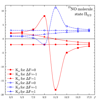
Figure 2: Sensitivity coefficients for $\Lambda$-doublet lines in $\Pi_{3/2}$ state of ¹⁵NO molecule. The difference between two hyperfine components with $\Delta F=0$ is too small to be seen. Sensitivity coefficients for $\Pi_{1/2}$ state correspond to the coupling case $a$ (see Eq. (11a)).

Now let us consider sensitivity coefficients for the molecule ¹⁵NO. Here we expect expressions for the coupling case $a$ to be applicable. In fact, for the state $\Pi_{1/2}$ coefficients $K_{\alpha}$ and $K_{\beta}$ agree with prediction (11a) within few percent and $K_{g}\ll 1$. However, for the state $\Pi_{3/2}$ Eq. (11b) works only for transitions with $\Delta F=0$, see Fig. 2. Indeed, $\Lambda$-splitting for low values of $J$ is smaller, than hyperfine structure. As a result, the frequencies of $\Delta F=\pm 1$ transitions strongly depend on the hyperfine parameters. For some values of $J$ these frequencies can be very small, because $\Lambda$-splitting and hyperfine splitting cancel each other. This leads to enhancement of sensitivity coefficients, similar to that, discussed in Ref. Flambaum (2006). Fig. 2 shows that for ¹⁵NO molecule such singularity takes place for $\Delta F=-1$ transition near $J=\tfrac{11}{2}$. For smaller values of $J$ the hyperfine contribution to transition frequency dominates over $\Lambda$-splitting. Sensitivity coefficients for this case are similar to those of the normal hyperfine transitions, i.e. $K_{\alpha}\approx 2$ and $K_{\beta}\approx K_{g}\approx 1$. For higher values of $J$ they approach the limit (11b). For $\Delta F=1$ transitions there is no singularity and sensitivities change smoothly between same limiting values. Finally, the hyperfine energy for the lines with $\Delta F=0$ is negligible and these lines are described by Eq. (11b) for all values of $J$.

Table 3: Frequencies (in MHz) and sensitivity coefficients for $\Lambda$-doublet lines in ¹⁴N¹⁶O. Experimental frequencies and their uncertainties are taken from Refs. Lovas et al. ; Chen et al. .

Level	$J$	$F$	$F^{\prime}$	$\omega$ (MHz)				$K_{\alpha}$	$K_{\beta}$	$K_{g}$	$K_{Q}$
				Exper.	Uncert.	Theory	Diff.
${}^{2}\Pi_{1/2}$	$0.5$	0.5	0.5	$205.9510$	$0.0002$	$205.96$	$-0.01$	$1.95$	$1.03$	$-0.73$	$0.00$
	$0.5$	0.5	1.5	$225.9357$	$0.0002$	$225.93$	$0.00$	$1.95$	$1.02$	$-0.58$	$0.00$
	$0.5$	1.5	0.5	$411.2056$	$0.0002$	$411.19$	$0.01$	$1.97$	$1.01$	$0.13$	$0.00$
	$0.5$	1.5	1.5	$431.1905$	$0.0002$	$431.16$	$0.03$	$1.97$	$1.01$	$0.17$	$0.00$
	$1.5$	0.5	0.5	$560.8538$	$0.0002$	$561.22$	$-0.37$	$1.97$	$1.02$	$-0.27$	$0.00$
	$1.5$	0.5	1.5	$587.7467$	$0.0002$	$587.54$	$0.21$	$1.97$	$1.01$	$-0.21$	$0.09$
	$1.5$	1.5	0.5	$624.6494$	$0.0002$	$624.93$	$-0.28$	$1.97$	$1.02$	$-0.14$	$-0.09$
	$1.5$	1.5	1.5	$651.5425$	$0.0002$	$651.25$	$0.29$	$1.97$	$1.01$	$-0.09$	$0.00$
	$1.5$	1.5	2.5	$693.8282$	$0.0002$	$693.88$	$-0.05$	$1.98$	$1.01$	$-0.02$	$-0.04$
	$1.5$	2.5	1.5	$758.9106$	$0.0002$	$758.66$	$0.25$	$1.97$	$1.01$	$0.06$	$0.04$
	$1.5$	2.5	2.5	$801.1963$	$0.0002$	$801.29$	$-0.10$	$1.98$	$1.01$	$0.11$	$0.00$
	$2.5$	3.5	3.5	$1160.7768$	$0.0003$	$1160.95$	$-0.18$	$1.98$	$1.01$	$0.08$	$0.00$
	$3.5$	4.5	4.5	$1514.768$	$0.001$	$1514.97$	$-0.20$	$2.00$	$1.00$	$0.07$	$0.00$
${}^{2}\Pi_{3/2}$	$1.5$	0.5	0.5			$0.81$		$-2.09$	$3.05$	$-0.11$	$0.00$
	$1.5$	1.5	1.5	$0.612$	$0.001$	$0.87$	$-0.25$	$-2.96$	$4.31$	$-0.06$	$0.00$
	$1.5$	2.5	2.5	$1.029$	$0.001$	$0.96$	$0.07$	$-1.94$	$2.83$	$0.05$	$0.00$
	$1.5$	0.5	1.5			$44.45$		$2.09$	$0.93$	$1.01$	$1.25$
	$1.5$	1.5	0.5	$46.464$	$0.003$	$46.12$	$0.34$	$1.92$	$1.00$	$0.96$	$1.19$
	$1.5$	1.5	2.5	$73.286$	$0.003$	$73.33$	$-0.05$	$2.10$	$0.96$	$1.02$	$-0.42$
	$1.5$	2.5	1.5	$74.931$	$0.003$	$75.15$	$-0.22$	$2.00$	$1.02$	$1.00$	$-0.41$
	$2.5$	1.5	1.5			$3.38$		$-2.08$	$3.04$	$-0.06$	$0.00$
	$2.5$	2.5	2.5	$3.121$	$0.001$	$3.54$	$-0.41$	$-2.36$	$3.44$	$-0.02$	$0.00$
	$2.5$	3.5	3.5	$3.923$	$0.001$	$3.75$	$0.17$	$-1.99$	$2.91$	$0.04$	$0.00$
	$2.5$	1.5	2.5			$27.37$		$2.64$	$0.70$	$1.14$	$-0.97$
	$2.5$	2.5	1.5	$34.39$	$0.03$	$34.28$	$0.11$	$1.68$	$1.17$	$0.90$	$-0.77$
	$2.5$	2.5	3.5	$40.172$		$40.07$	$0.10$	$2.46$	$0.76$	$1.08$	$0.46$
	$2.5$	3.5	2.5	$47.211$	$0.001$	$47.36$	$-0.14$	$1.77$	$1.11$	$0.92$	$0.39$
	$3.5$	2.5	2.5			$8.58$		$-2.07$	$3.03$	$-0.04$	$0.00$
	$3.5$	3.5	3.5			$8.88$		$-2.07$	$3.03$	$-0.01$	$0.00$
	$3.5$	4.5	4.5			$9.26$		$-2.07$	$3.03$	$0.03$	$0.00$
	$3.5$	2.5	3.5			$13.59$		$5.06$	$-0.39$	$1.73$	$-6.83$
	$3.5$	3.5	2.5	$31.550$	$0.004$	$31.05$	$0.50$	$1.03$	$1.51$	$0.73$	$-2.94$
	$3.5$	3.5	4.5			$21.54$		$3.90$	$-0.01$	$1.38$	$3.32$
	$3.5$	4.5	3.5	$39.221$	$0.002$	$39.67$	$-0.45$	$1.18$	$1.40$	$0.76$	$1.82$
	$4.5$	3.5	3.5			$17.25$		$-2.05$	$3.02$	$-0.03$	$0.00$
	$4.5$	4.5	4.5			$17.74$		$-2.05$	$3.02$	$-0.01$	$0.00$
	$4.5$	5.5	5.5			$18.33$		$-2.05$	$3.03$	$0.03$	$0.00$
	$4.5$	3.5	4.5			$0.96$		$-80.19$	$38.95$	$-19.07$	$157.32$
	$4.5$	4.5	3.5	$35.045$	$0.002$	$34.02$	$1.02$	$0.16$	$1.95$	$0.50$	$-4.33$
	$4.5$	4.5	5.5			$5.26$		$16.68$	$-6.81$	$4.16$	$23.52$
	$4.5$	5.5	4.5	$40.512$	$0.001$	$41.33$	$-0.81$	$0.34$	$1.81$	$0.55$	$3.05$

Table 4: Frequencies (in MHz) and sensitivity coefficients for $\Lambda$-doublet lines in ⁷Li¹⁶O. Experimental frequencies and their uncertainties are taken from Ref. Lovas et al. .

Level	$J$	$F$	$F^{\prime}$	$\omega$ (MHz)				$K_{\alpha}$	$K_{\beta}$	$K_{g}$	$K_{Q}$
				Exper.	Uncert.	Theory	Diff.
${}^{2}\Pi_{3/2}$	$1.5$	1	1	$11.28$	$0.01$	$11.18$	$0.10$	$-1.90$	$2.94$	$0.00$	$0.00$
	$1.5$	2	2	$11.28$	$0.01$	$11.18$	$0.10$	$-1.90$	$2.94$	$0.00$	$0.00$
	$1.5$	3	3	$11.28$	$0.01$	$11.19$	$0.09$	$-1.90$	$2.94$	$0.00$	$0.00$
	$1.5$	0	1			$9.82$		$-2.51$	$3.25$	$-0.14$	$0.63$
	$1.5$	1	0			$12.53$		$-1.46$	$2.74$	$0.11$	$-0.49$
	$1.5$	1	2	$8.55$	$0.10$	$8.41$	$0.14$	$-3.26$	$3.59$	$-0.33$	$0.72$
	$1.5$	2	1	$14.00$	$0.05$	$13.95$	$0.05$	$-1.07$	$2.55$	$0.20$	$-0.44$
	$1.5$	2	3	$6.95$	$0.05$	$6.87$	$0.08$	$-4.47$	$4.24$	$-0.61$	$-0.89$
	$1.5$	3	2	$15.60$	$0.02$	$15.50$	$0.10$	$-0.76$	$2.36$	$0.27$	$0.40$
	$2.5$	1	1	$45.02$	$0.03$	$44.80$	$0.22$	$-1.90$	$2.95$	$0.00$	$0.00$
	$2.5$	2	2	$45.02$	$0.03$	$44.80$	$0.22$	$-1.90$	$2.95$	$0.00$	$0.00$
	$2.5$	3	3	$45.02$	$0.03$	$44.81$	$0.21$	$-1.90$	$2.95$	$0.00$	$0.00$
	$2.5$	4	4	$45.02$	$0.03$	$44.83$	$0.19$	$-1.90$	$2.95$	$0.00$	$0.00$
	$2.5$	1	2	$44.04$	$0.03$	$43.82$	$0.22$	$-2.01$	$3.01$	$-0.02$	$-0.08$
	$2.5$	2	1	$45.97$	$0.03$	$45.78$	$0.19$	$-1.81$	$2.90$	$0.02$	$0.08$
	$2.5$	2	3	$43.60$	$0.03$	$43.37$	$0.23$	$-2.06$	$3.03$	$-0.03$	$-0.05$
	$2.5$	3	2	$46.43$	$0.03$	$46.24$	$0.19$	$-1.76$	$2.88$	$0.03$	$0.04$
	$2.5$	3	4	$43.17$	$0.03$	$42.97$	$0.20$	$-2.11$	$3.06$	$-0.04$	$0.08$
	$2.5$	4	3	$46.86$	$0.03$	$46.67$	$0.19$	$-1.71$	$2.86$	$0.04$	$-0.08$
	$3.5$	3	3	$112.237$	$0.002$	$112.28$	$-0.04$	$-1.91$	$2.96$	$0.00$	$0.00$
	$4.5$	4	4	$223.756$	$0.003$	$225.24$	$-1.48$	$-1.91$	$2.99$	$0.00$	$0.00$
${}^{2}\Pi_{1/2}$	$0.5$	1	1			$2958.44$		$2.10$	$0.95$	$0.00$	$0.00$
	$0.5$	2	2			$2969.20$		$2.10$	$0.95$	$0.00$	$0.00$
	$0.5$	1	2			$2947.37$		$2.10$	$0.95$	$-0.01$	$0.00$
	$0.5$	2	1			$2980.27$		$2.10$	$0.95$	$0.01$	$0.00$
	$1.5$	1	1			$5971.29$		$2.10$	$0.96$	$0.00$	$0.00$
	$1.5$	2	2			$5975.59$		$2.10$	$0.96$	$0.00$	$0.00$
	$1.5$	3	3			$5982.05$		$2.10$	$0.96$	$0.00$	$0.00$
	$1.5$	1	2			$5969.71$		$2.10$	$0.96$	$0.00$	$0.00$
	$1.5$	2	1			$5977.18$		$2.10$	$0.96$	$0.00$	$0.00$
	$1.5$	2	3			$5973.38$		$2.10$	$0.96$	$0.00$	$0.00$
	$1.5$	3	2			$5984.26$		$2.10$	$0.96$	$0.00$	$0.00$
	$2.5$	2	2			$9078.46$		$2.11$	$0.97$	$0.00$	$0.00$
	$3.5$	2	2	$12321.51$	$0.03$	$12322.14$	$-0.63$	$2.13$	$0.99$	$0.00$	$0.00$
	$3.5$	3	3	$12325.82$	$0.03$	$12325.21$	$0.61$	$2.13$	$0.99$	$0.00$	$0.00$
	$3.5$	2	3	$12319.93$	$0.03$	$12321.60$	$-1.67$	$2.13$	$0.99$	$0.00$	$0.00$
	$3.5$	3	2	$12327.41$	$0.03$	$12325.75$	$1.66$	$2.13$	$0.99$	$0.00$	$0.00$

The spectrum and sensitivity coefficients of the molecule ¹⁴NO are similar to those of ¹⁵NO. Because ¹⁴N has nuclear spin $I=1$, the hyperfine structure of the $\Lambda$-doublet lines is more complex and consists of up to 7 hyperfine components. Hyperfine Hamiltonian includes magnetic dipole part (14) and electric quadrupole part (15) and is described by five hyperfine parameters, which we take from Ref. Lovas et al. . As we said above, we are not discussing nuclear theory here and consider nuclear quadrupole moment as independent FC. Because of that $\Lambda$-doublet spectrum is now described by four sensitivity coefficients (see Table 3).

Sensitivity coefficients $K_{\alpha}$ and $K_{\beta}$ of the $\Lambda$-doublet lines of the state $\Pi_{1/2}$ again agree with (11a) within few percent. The lowest frequency transitions for $J=\tfrac{1}{2}$ have sensitivity coefficients $K_{g}$ of the order of unity, but they rapidly decrease with frequency and with $J$. Coefficients $K_{Q}$ for the state $\Pi_{1/2}$ are always small.

For the state $\Pi_{3/2}$ there are transitions of three types. First type transitions correspond to $\Delta F=0$. The hyperfine energy difference here is small compared to $\Lambda$-splitting. These transitions have sensitivity coefficients $K_{\alpha}$ and $K_{\beta}$ close to prediction (11b) and small coefficients $K_{g}$ and $K_{Q}$. Second type transitions correspond to $\Delta F=\pm 1$ and small values of $J$. Hyperfine energy for these transitions dominates over $\Lambda$-splitting. Sensitivity coefficients here are close to those of pure hyperfine transitions, i.e. $K_{\alpha}=2$ and $K_{\beta}=1$. As long as hyperfine energy includes comparable magnetic dipole and electric quadrupole parts, coefficients $K_{g}$ and $K_{Q}$ are of the order of unity, but may significantly differ from one transition to another. Note that all transitions of this type for ¹⁵NO molecule have $K_{g}\approx 1$.

Transitions of the third type also correspond to $\Delta F=\pm 1$, but higher rotational quantum numbers $J=\tfrac{7}{2},\,\tfrac{9}{2}$. The hyperfine transition energy here is comparable to $\Lambda$-splitting and they can either double, or almost cancel each other. Consequently, sensitivity coefficient are widely spread and can become very large for transitions with anomalously low frequency.

Note that low frequency transitions for $J=\tfrac{9}{2}$ were not observed experimentally and we use theoretical frequencies to calculate sensitivity coefficients. Because of significant cancelation of different contributions, the accuracy of these frequencies can be low. When these frequencies are measured, respective sensitivity coefficients should be corrected:

$$K_{i,\mathrm{cor}}=K_{i}\frac{\omega_{\mathrm{theor}}}{\omega_{\mathrm{exper}}}$$ (16)

Sensitivity coefficients for LiO molecule are listed in Table 4. The hyperfine structure here is smaller than for NO molecule and sensitivity coefficients are closer to case $a$ values (11a,11b). Significant deviations are found only for $J=\tfrac{3}{2},\,\Delta F=\pm 1$ transitions of $\Pi_{3/2}$ state. Also, these are the only transitions, where coefficients $K_{g}$ and $K_{Q}$ are not negligible. For this molecule there are no transitions with anomalously small frequencies and, therefore, sensitivity coefficients are not enhanced.

IV Conclusions

In this paper we calculated sensitivity coefficients to variation of fundamental constants for $\Lambda$-doublet spectra of several light diatomic molecules. We found several lines with anomalously high sensitivity. All these lines have relatively low frequencies and enhanced sensitivity is caused by the significant cancelations between contributions from different parts of the effective Hamiltonian (12).

In CH and OH molecules enhancement takes place when electron spin decouples from the molecular axis and $\Omega$-doubling is transformed into $\Lambda$-doubling. For one of the two states $\Pi_{1/2}$, or $\Pi_{3/2}$ this transformation leads to the change of sign of the splitting between states with definite parity and enhanced sensitivity to FC variation.

Rotational constant $B$ for ¹⁴NO and ¹⁵NO molecules is much smaller, than for CH and NH molecules and electron spin is strongly coupled to the axis. Consequently, there is no enhancement caused by decoupling. On the other hand, the hyperfine structure of the $\Lambda$-doublet lines is comparable to $\Lambda$-splitting in $\Pi_{3/2}$ state. For some transition lines with $\Delta F=\pm 1$ the hyperfine energy almost cancel $\Lambda$-splitting leading to enhanced sensitivity.

For LiO molecule electron spin is strongly coupled to the axis and hyperfine structure is smaller than $\Lambda$-splitting. As a result, there is no strong enhancement of the sensitivity to FC variation. However, even here sensitivity coefficients strongly depend on the quantum numbers.

Sensitivity coefficients for $\Lambda$-doublet transitions of OH molecules were calculated before in Refs. Kanekar et al. (2005); Kanekar and Chengalur (2004). For all these states our results are in good agreement with those calculations. In particular, from Table 2 we find sensitivity coefficients for the 18 cm ground state $\Lambda$-doublet transitions with $J=\tfrac{3}{2}$ and $F^{\prime}=F$ to be: $K_{\alpha}=-1.14$, $K_{\beta}=2.55$, and $K_{g}=0$. In the the paper Kanekar et al. (2005) the 21-cm Hydrogen line was used as a reference. It has $K_{\alpha}=2$, $K_{\beta}=1$, and $K_{g}=1$. Parameter $\cal F$ according to Eq. (5) is given by the expression:

$${\cal F}=\alpha^{\Delta K_{\alpha}}\beta^{\Delta K_{\beta}}g_{\mathrm{nuc}}^{\Delta K_{g}}=\alpha^{3.14}\beta^{-1.55}g_{\mathrm{nuc}}^{1}\,.$$ (17)

This result is sufficiently close to Eq. (1).

For astrophysical observations it is important to have accurate laboratory measurements so that frequency ratios for distant object can be compared to the respective local ratios. Sufficiently accurate frequency measurements were done only for 18 cm lines of OH Lev et al. (2006); Hudson et al. (2006) and for 9 cm lines of CH McCarthy et al. (2006). These lines can be used for new studies of the variation of FC without significant preliminary work. For other lines at present there are no sufficiently accurate laboratory frequencies. New laboratory measurements are necessary before these lines can be used for our purposes. In particular, the hyperfine components of the 42 cm CH line are most interesting as they have high sensitivity to both fundamental constants and were already observed in astrophysics for distant objects.

In principle it is possible to study time variation of FC without referring to the laboratory measurements. For this purpose it is possible to compare microwave spectra for molecular clouds from our Galaxy with extragalactic spectra of the same species. In many cases the line widths for the galactic spectra are one-two orders of magnitude smaller, than for objects at cosmological distances, so they can serve as very good reference.

Let us briefly discuss the feasibility of the laboratory tests of time-variation of FC using molecular $\Lambda$-doublets. Present model independent laboratory limit on $\beta$-variation is Shelkovnikov et al. (2008):

$$\frac{\mathrm{d}\beta/\mathrm{d}t}{\beta}=(3.8\pm 5.6)10^{-14}\,\mathrm{yr}^{-1}\,,$$ (18)

and the limit on $\alpha$-variation is three orders of magnitude stronger, on the level $10^{-17}$ Rosenband et al. (2008). To improve constrained (18) one needs to measure frequency shifts $\delta\omega<K_{\beta}\omega\delta\beta/\beta$. For the 18 cm OH line this corresponds to the shift $\delta\omega\lesssim 4\times 10^{-4}$ Hz. This is few orders of magnitude smaller than the accuracy of the best present measurements Lev et al. (2006); Hudson et al. (2006). On the other hand, at present there is rapid progress in precision molecular spectroscopy caused by development of sources of ultracold molecules (see review Carr et al. (2009) and references therein). Thus it is possible that molecular tests of FC variation using $\Lambda$-doublet lines can become competitive in the near future.

When comparing sensitivity of different laboratory experiments on time-variation it is not sufficient to look for large dimensionless sensitivity coefficients (3). In high precision laboratory measurements the line widths are not dominated by the Doppler effect and are not proportional to the frequency. Because of that, instead of the dimensionless sensitivity coefficients $K_{i}$, which determine relative frequency shifts (3), one has to look for large absolute sensitivities $K_{i}\omega$, which determine absolute frequency shifts $\delta\omega$ and for narrow lines. In astrophysics, on the contrary, all lines are Doppler-broadened and dimensionless sensitivity coefficients $K_{i}$ become crucial.