Mesoscopic quantum switching of a Bose-Einstein condensate in an optical lattice governed by the parity of the number of atoms

Abstract

It is shown that for a $N$-boson system the parity of $N$ can be responsible for a qualitative difference in the system response to variation of a parameter. The nonlinear boson model is considered, which describes tunneling of boson pairs between two distinct modes $X_{1,2}$ of the same energy and applies to a Bose-Einstein condensate in an optical lattice. By varying the lattice depth one induces the parity-dependent quantum switching, i.e. $X_{1}\to X_{2}$ for even $N$ and $X_{1}\to X_{1}$ for odd $N$, for arbitrarily large $N$. A simple scheme is proposed for observation of the parity effect on the mesoscopic scale by using the bounce switching regime, which is insensitive to the initial state preparation (as long as only one of the two $X_{l}$ modes is significantly populated), stable under small perturbations and requires an experimentally accessible coherence time.

Mesoscopic quantum phenomena lie in between the big and small: the macroscopic classical world and the microscopic quantum world. The Bose-Einstein condensate (BEC) is such a mesoscopic effect, i.e. a big “matter-wave”. An order parameter governed by the Gross-Pitaevskii equation Legg ; PS ; MF is usually attributed to BEC. The order parameter corresponds to the mean-field theory, i.e. to the limit of large number of bosons: $N\to\infty$ at a constant density. The latter, on the other hand, is equivalent to the classical limit of the discrete WKB approach Braun , with $1/N$ playing the role of the Planck constant (see, for instance, Refs. SK1 ; SK2 ).

The mean-field limit is a singular limit of the full quantum description and suffers from deficiency, e.g. at a dynamic instability MF , due to the back-reaction of the quantum fluctuations AV , or the appearance of the Schrödinger cat-like states WT . In this connection one can mention the “even-odd” effect, first predicted for the spin systems Spar and observed in the small ($S\sim 10$) magnetic molecular clusters as the parity-dependent tunneling splitting SparExp . The parity effect was also found in the decay of the Josephson $\pi$-states Jpi and in the boson-Josephson model BEC2w . The tunneling splitting, however, decreases exponentially in $N$, for $N\gg 1$, restricting its observation to the sub-mesoscopic scale. One may wonder whether it is possible to magnify the microscopic parity difference to a mesoscopic scale and how? Such an effect would be also an interesting manifestation of the singularity in the $N\to\infty$ limit of the discrete WKB.

The aim of this rapid communication is to present a solution: one must look for a dynamic parity effect which allows for a massive constructive quantum interference. Moreover, the feasibility of the experimental observation is shown. The mesoscopic parity effect appears in the response to variation of a parameter in the nonlinear two-mode boson model SK1 , a nonlinear variant of the celebrated boson-Josephson model bJ ; SKPRL .

The nonlinear two-mode boson model is formulated as follows. Suppose that a single-particle Hamiltonian $H_{0}$ has two equal energy states $X_{1}$ and $X_{2}$ and that the interaction term $H_{\mathrm{int}}=\frac{g}{2}\int\mathrm{d}^{3}{\bf x}\psi^{\dagger}({\bf x})\psi^{\dagger}({\bf x})\psi({\bf x})\psi({\bf x})$ in the many-body Hamiltonian $H=\int\mathrm{d}^{3}{\bf x}\psi^{\dagger}({\bf x})H_{0}\psi({\bf x})+H_{\mathrm{int}}$ is smaller than the energy gap of $H_{0}$ isolating the resonant subspace. Projecting on the resonant states, $\psi({\bf x})=b_{1}\varphi_{X_{1}}({\bf x})+b_{2}\varphi_{X_{2}}({\bf x})$, one arrives at the Hamiltonian: $H_{\mathrm{int}}=\frac{g}{2}\left\{\sum\chi_{i_{1},i_{2},j_{1},j_{2}}b^{\dagger}_{i_{1}}b^{\dagger}_{i_{2}}b_{j_{1}}b_{j_{2}}\right\}$, ${i_{1},i_{2},j_{1},j_{2}}\in\{1,2\}$, where $\chi_{i_{1},i_{2},j_{1},j_{2}}\equiv\int\mathrm{d}^{3}{\bf x}\,\varphi^{*}_{X_{i_{1}}}\varphi^{*}_{X_{i_{2}}}\varphi_{X_{j_{1}}}\varphi_{X_{j_{2}}}$. We consider the situation when the bosons hop between the modes $X_{l}$ by pairs, i.e. when $\chi_{12jj}=0$ for $j=1,2$. This type of coupling describes the intraband tunneling of BEC in a square optical lattice SK1 , where the resonant modes are the high-symmetry points of the Brillouin zone, $X_{1}=(k_{B},0)$ and $X_{2}=(0,k_{B})$, and the quasimomentum conservation makes $\chi_{12jj}$ vanish. Moreover, it also applies to BEC on a rotated ring lattice RL . The intraband BEC tunneling Hamiltonian reads

$$\hat{H}=\frac{1}{2N^{2}}\left\{n_{1}^{2}+n_{2}^{2}+\Lambda\left[4n_{1}n_{2}+(b_{1}^{\dagger}b_{2})^{2}+(b_{2}^{\dagger}b_{1})^{2}\right]\right\},$$ (1)

where $n_{j}=b^{\dagger}_{j}b_{j}$ and $\Lambda=\chi_{1122}/\chi_{1111}$ ($0\leq\Lambda\leq 1$) is the only parameter in the model (see for details Ref. SK1 ; SKPRL ). The corresponding Schrödinger equation is cast as $ih\partial_{\tau}|\Psi\rangle=\hat{H}|\Psi\rangle$, where $h=2/N$ is the effective Planck constant and the dimensionless time $\tau=(2gN\chi_{1111}/\hbar)t$, with $g=4\pi\hbar^{2}a_{s}/m$, depends on $N$ through the density only.

Hamiltonian (1) features SKPRL a quantum phase transition at the top of the spectrum related to the mean-field symmetry-breaking bifurcation between the stationary point $(\langle b^{\dagger}_{1}b_{1}\rangle/N=1/2,\phi\equiv\arg\langle(b_{2}^{\dagger})^{2}b_{1}^{2}\rangle=0)$, corresponding to the equally populated $X_{l}$ modes, which is stable for $\Lambda>\Lambda_{c}=1/3$, and the selftrapping stationary points ($\langle b^{\dagger}_{1}b_{1}\rangle/N\ll 1$ or $\langle b^{\dagger}_{2}b_{2}\rangle/N\ll 1$, $\phi$ undefined), stable for $\Lambda<\Lambda_{c}$. It also has a parity-dependent energy spectrum (see also Fig 1(a)). There are two invariant subspaces corresponding to the even and odd occupation numbers $k$ in the Fock basis, i.e. $|\Psi\rangle=\sum_{k=0}^{N}C_{k}|k,N-k\rangle$, with $|k,N-k\rangle\equiv\frac{(b^{\dagger}_{1})^{k}(b^{\dagger}_{2})^{N-k}}{\sqrt{k!(N-k)!}}|\mathrm{vac}\rangle$. The projections of $\hat{H}$ on the even ($\mathrm{s}=0$ or “ev”) and odd ($\mathrm{s}=1$ or “od”) subspace are given as

$$H^{(\mathrm{s})}=\begin{pmatrix}{\alpha}_{s}&{\beta}_{s+1}&0&\ldots&0\\ {\beta}_{s+1}&{\alpha}_{s+2}&\ddots&\ddots&\vdots\\ 0&\ddots&\ddots&\ddots&0\\ \vdots&\ddots&\ddots&\ddots&{\beta}_{2L-1-s}\\ 0&\ldots&0&{\beta}_{2L-1-s}&{\alpha}_{2L-s}\end{pmatrix},$$ (2)

where, respectively for even and odd $N$: $L=N/2$ and $L=(N-1)/2$ in the case of $H^{(\mathrm{ev})}$, while $L=N/2$ and $L=(N+1)/2$ in the case of $H^{(\mathrm{od})}$. Here ${\alpha}_{k}=(2\Lambda-1)\frac{k}{N}\left(1-\frac{k}{N}\right)$ and ${\beta}_{k}=\frac{\Lambda}{2}\left[\frac{k}{N}\left(\frac{k}{N}+\frac{1}{N}\right)\left(1-\frac{k}{N}\right)\left(1-\frac{k}{N}+\frac{1}{N}\right)\right]^{1/2}$.

When $N$ is odd we have $PH^{(\mathrm{ev})}P=H^{(\mathrm{od})}$, where $P=\mathrm{diag}(1,\ldots,1)^{T}$ (i.e. the transposed $\openone$). In this case $P|E^{(\mathrm{ev})}_{j}\rangle=|E^{(\mathrm{od})}_{j}\rangle$, i.e. the energy levels are doubly degenerate. On the other hand, this is a consequence of the Kramers theorem KTh . Indeed, Hamiltonian (1) is equivalent to a spin model $H_{S}=(1-\Lambda)S^{2}_{z}+2\Lambda S^{2}_{x}$ with the total spin $S=N/2$, if we associate $S_{x}=(b^{\dagger}_{1}b_{2}+b^{\dagger}_{2}b_{1})/2$, $S_{y}=(b^{\dagger}_{1}b_{2}-b^{\dagger}_{2}b_{1})/2i$ and $S_{z}=(b^{\dagger}_{1}b_{1}-b^{\dagger}_{2}b_{2})/2$.

When $N$ is even the projected Hamiltonian $H^{(\mathrm{s})}$ is invariant under the exchange symmetry, i.e. $PH^{(\mathrm{s})}P=H^{(\mathrm{s})}$, $\mathrm{s}\in\{\mathrm{0,\;1\}}$. One control parameter can not cause the energy level degeneracy NW , thus the eigenvectors of $H^{(\mathrm{s})}$ must satisfy the exchange symmetry, namely $P|E^{(\mathrm{s})}_{j}\rangle=(-1)^{j+\frac{N}{2}+1-s}|E^{(\mathrm{s})}_{j}\rangle$, $j=1,\ldots,\frac{N}{2}+1-s$. For a finite $\Lambda_{c}-\Lambda>0$ the eigenvalues of $H^{(\mathrm{s})}$ appear in the form of very narrow doublets (see also Fig. 1(a)) due to the “selftrapping states” being strongly localized at the respective $X_{l}$ mode (e.g. typically $|\langle k,N-k|\Psi\rangle|^{2}\leq 10^{-6}$ for $k>25$ SKPRL ). Consequently, each $H^{(\mathrm{s})}$ also has the quasi-degenerate spectra (since $H^{(\mathrm{ev})}-H^{(\mathrm{od})}\propto\frac{1}{N}$) which become finer for larger deviations $\Lambda_{c}-\Lambda$, exactly as the numerics indicates.

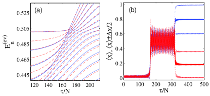
Figure 1: (Color online) Panel (a): the energy level structure of $H^{(\mathrm{ev})}$ for $N=40$ (solid lines) and $41$ (dashed lines). Panel (b): the average ratio of the $X_{1}$-mode occupation number $\langle x\rangle=\langle b_{1}{\!\!}^{\dagger}b_{1}\rangle/N$ (dark solid lines) and $\langle x\rangle-\frac{\Delta x}{2}$, $\langle x\rangle+\frac{\Delta x}{2}$ (light dashed lines), with $\Delta x=\langle(b_{1}{\!\!}^{\dagger}b_{1}/N-\langle x\rangle)^{2}\rangle^{1/2}$. The upper lines (solid and dashed) correspond to $N=40$ and the lower ones to $N=41$. The initial state is a Gaussian $|\Psi\rangle=A_{\sigma}\sum_{k=0}^{N}e^{-k^{2}/\sigma^{2}}|k,N-k\rangle$, where $\sigma=4$. Here $\Lambda(\tau)=\Lambda_{1}+1/2(\Lambda_{2}-\Lambda_{1})\left[\tanh\left(\kappa[\tau-\tau_{1}]\right)-\tanh\left(\kappa[\tau-\tau_{2}]\right)\right]$ with $\kappa=10^{-4}$, $\tau_{1}=7000$ and $\tau_{2}=12800$.

Consider now the following experimentally realizable setup: initially just one of the $X_{l}$ modes is significantly populated (to achieve this one can use the non-adiabatic loading Blochload into one of the two resonant Bloch states of the lattice with $\Lambda_{1}<1/3$). By varying the lattice parameter (e.g. by changing the lattice depth) between $\Lambda_{1}$ and $\Lambda_{2}$, with $\Lambda_{2}>\Lambda_{c}$, one drives the system across the phase transition and back to force a switching-like dynamics between the selftrapping states at the $X_{l}$ modes. Remarkably, for a general initial state localized at just one $X_{l}$ mode, e.g. $|\Psi\rangle=\sum_{k=0}^{K\ll N}C_{k}|k,N-k\rangle$, where the distribution $C_{k}$ is not important, the result qualitatively depends on the parity of $N$, see Fig. 1(b). Note that the switching is between the Bloch modes with orthogonal Bloch vectors: $X_{1}=(k_{B},0)$ and $X_{2}=(0,k_{B})$.

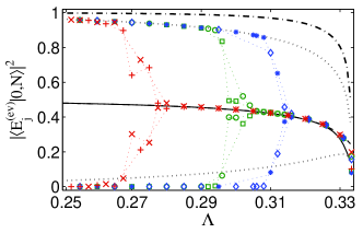
Figure 2: (Color online) The probabilities $|\langle E^{(\mathrm{ev})}_{j}|0,N\rangle|^{2}$, $j=L+1$ and $j=L$, given for $N=40$ by the solid and dashed lines (almost coincide), for $N=60$ by the “$+$” and “$\times$”, for $N=80$ by the “$\square$” and “$\circ$” and for $N=100$ by the “$*$” and “$\diamond$” symbols. The upper dash-dotted line gives $\sum_{m=0}^{3}|\langle E^{(\mathrm{ev})}_{L+1-m}|0,N\rangle|^{2}$. The upper and lower dotted lines give, respectively, $|\langle E^{(\mathrm{ev})}_{L+1}|0,N\rangle|^{2}$ and $\sum_{m=1}^{3}|\langle E^{(\mathrm{ev})}_{L+1-m}|0,N\rangle|^{2}$ for odd $N$. The data, connected by the dotted lines to guide the eye, that lie off the central curve are due to the quasi-degeneracy on the order of round-off error.

In the adiabatic limit the mechanism of the switching for a localized initial distribution $C_{k}$ can be understood by considering separately the even and odd invariant subspaces. For simplicity, consider the initial state $|\Psi\rangle=|0,N\rangle\in H^{(\mathrm{ev})}$ (the case of $|\Psi\rangle=|1,N-1\rangle\in H^{(\mathrm{od})}$ is similar). Fig. 2 shows that there are but few significant terms (from the top of the spectrum) in the expansion of the initial state over the eigenvectors (recall the strong localization of the eigenvectors at $k=0$ and $k=N$ for $\Lambda<\Lambda_{c}$). For even $N$ there are the quantum beats, i.e. oscillations of the populations, between the successive pairs of eigenstates from the top of the energy spectrum. This can be understood as tunneling between the $X_{l}$ modes. The switching occurs for the odd-$\pi$ phase differences between the first few pairs of the successive top energy eigenstates, i.e. $\Delta\theta_{L+1-2j}\equiv\frac{1}{h}\int\limits_{0}^{\tau}\mathrm{d}t\,[E^{(\mathrm{s})}_{L+1-2j}(t)-E^{(\mathrm{s})}_{L-2j}(t)]\approx(2m_{j}-1)\pi$, $j=0,1,...\,$. For odd $N$, on the other hand, the eigenvectors break the $P$-symmetry and only those localized at $X_{1}$ acquire nonzero amplitudes (i.e. no tunneling). Thus, a high visibility parity effect requires at least few top dynamic phase differences in both the even and odd subspaces (for even $N$) to be odd in $\pi$, which, in the general case, can not be satisfied by adjusting $\tau_{2}-\tau_{1}$ in Fig. 1.

The Landau-Zener-Majorana (LZM) transitions between the instantaneous energy levels occur for the non-adiabatic variation of $\Lambda$. In the instantaneous eigenvector basis, $|\Psi^{(\mathrm{s})}(\tau)\rangle=\sum_{j}c_{j}(\tau)\exp\left[-\frac{i}{h}\int\limits_{0}^{\tau}\mathrm{d}t\,E^{(\mathrm{s})}_{j}(t)\right]|E^{(\mathrm{s})}_{j}(\tau)\rangle$, we have

$$\frac{\mathrm{d}c_{j}}{\mathrm{d}\tau}=\frac{\mathrm{d}\Lambda}{\mathrm{d}\tau}\sum_{l\neq j}c_{l}\frac{\langle E^{(\mathrm{s})}_{j}|\frac{\mathrm{d}\hat{H}}{\mathrm{d}\Lambda}|E^{(\mathrm{s})}_{l}\rangle}{E^{(\mathrm{s})}_{j}-E^{(\mathrm{s})}_{l}}e^{-\frac{i}{h}\int\limits_{0}^{\tau}\mathrm{d}t\,[E^{(\mathrm{s})}_{j}-E^{(\mathrm{s})}_{l}]},$$ (3)

where it was used that $\langle E^{(\mathrm{s})}_{j}|\frac{\mathrm{d}}{\mathrm{d}\tau}|E^{(\mathrm{s})}_{j}\rangle=0$ ($H^{(\mathrm{s})}$ does not have energy degeneracy). Due to the exchange symmetry $P$, in the even $N$ case the LZM tunneling occurs only between the levels $E^{(\mathrm{s})}_{j}$ with the same parity of $j$, whereas for odd $N$ there is a small coupling also between the adjacent levels, since $H^{(\mathrm{s})}_{2L+1}-H^{(\mathrm{s})}_{2L}\propto\frac{1}{N}$. The LZM result LZM states that $|c_{l}|^{2}\sim\exp\left(-\frac{\pi(\Delta E)^{2}}{h\left(\frac{\mathrm{d}\Delta E}{\mathrm{d}\tau}\right)}\right)$, for $l\neq j$. Hence, the lower limit on the adiabatic time scale, i.e. $|c_{l}|^{2}\ll 1$, can be determined from the difference between the top energy levels $E^{(\mathrm{s})}_{n+1}-E^{(\mathrm{s})}_{n}\propto\frac{1}{N^{2}}$ for $\Lambda\to\Lambda_{c}$ SKPRL (see also below). We get $\tau_{\mathrm{ad}}\gg N$ (the time scale for a finite phase difference $\Delta\theta_{j}$ is $\tau_{\mathrm{ph}}\sim N$, since $h=2/N$). Therefore, the adiabatic case also requires an extremely long coherence time and thus it is not realistic at all.

In the other limit, Fig. 3, when $\Lambda(\tau)$ is a step-like function (e.g. similar to the one used in Fig. 1(b), but with $\kappa\sim 1$ or larger) taking two values $\Lambda_{1}<\Lambda_{c}$ and $\Lambda_{2}=\Lambda_{c}$, the switching regime, the bounce switching for below, has all the needed properties.

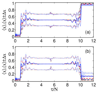
Figure 3: (Color online) The bounce switching for the initial state $|\Psi\rangle=A_{\sigma}\sum_{k=0}^{N}e^{-k^{2}/\sigma^{2}}|k,N-k\rangle$. Panel (a) $N=200$ and panel (b) $N=201$. In both panels, the average ratio $\langle x\rangle$ (the thick lines) with the side lines $\langle x\rangle-\frac{\Delta x}{2}$ and $\langle x\rangle+\frac{\Delta x}{2}$ (the thin lines) are given for $\sigma=0.05N$ (dash-dotted lines), $\sigma=0.1N$ (dashed lines), and $\sigma=0.2N$ (solid lines). Here $\Lambda(\tau)$ is as in Fig. 1 with $\kappa=8$, $\Lambda_{1}=0.25$, $\Lambda_{2}=1/3$, and $\tau_{2}-\tau_{1}=3N\pi$.

Indeed, the bounce switching possesses the $N$-scaling property, thus it survives in the $N\to\infty$ limit, and is insensitive to the initial distribution $C_{k}$ (localized at just one $X$-mode). These features originate from the fact that all the dynamic phases are odd in $\pi$. Indeed, Hamiltonian (1) in the coherent basis $a_{1,2}=(b_{1}\mp ib_{2})/\sqrt{2}$ reads $\hat{H}=\frac{2\Lambda}{N^{2}}a^{\dagger}_{1}a_{1}a^{\dagger}_{2}a_{2}+\frac{1-3\Lambda}{4N^{2}}\left(a_{1}^{\dagger}a_{2}+a_{2}^{\dagger}a_{1}\right)^{2}+\mathrm{const}$ with the energies $E_{\ell}(\Lambda_{c})=\frac{2}{3N^{2}}(\ell-1)(N-\ell+1)$, $\ell=1,...,\left[\frac{N}{2}\right]+1$. Hence, the dynamic phase differences are given as $\Delta\theta^{(\mathrm{s})}_{L+1-s-2n}=\frac{4n+2s+1}{3N}\Delta\tau_{c}$, $n=0,1,2,\ldots$, where $\Delta\tau_{c}$ is the hold time at $\Lambda_{c}$. By setting $\Delta\tau_{c}=3\pi N$ one obtains $\Delta\theta^{(\mathrm{s})}_{L+1-s-2n}=(4n+2s+1)\pi$.

The actual physical time, $t=t_{\mathrm{ph}}\frac{\tau}{N}$ with $t_{\mathrm{ph}}\equiv\frac{\hbar}{2g\chi_{1111}}$, is $N$-independent due to the scaling property $\Delta\tau_{c}=3\pi N$. For a condensate in a square lattice of $n$ cites of size $d$ in the tight transverse trap with the oscillator length $a_{\perp}$ the coherence time is $\Delta t\sim\frac{md^{2}a_{\perp}n}{\hbar a_{s}}$. For ⁸⁷Rb, $n=64$, $d=0.5\mu$m and $a_{\perp}=0.1\mu$m the required coherence time is $\Delta t\sim 0.3\,\mathrm{s}$. The switching can be detected by releasing the optical lattice and observing the direction of the interference pattern. For the lattice $V=V_{0}\left[\cos(2k_{B}x)+\cos(2k_{B}y)\right]$ the parameter range is $V_{0}=0.58E_{R}$ for $\Lambda=0.25$ and $V_{0}=0.3573E_{R}$ for $\Lambda=1/3$. Finally, the applicability condition for the two-mode model $E_{\mathrm{NL}}/E_{R}\ll 1$, where $E_{R}\equiv\hbar^{2}k_{B}^{2}/2m$ and $E_{\mathrm{NL}}\equiv gN\chi_{1111}$, can be cast as $N\ll na_{\perp}/a_{s}$.

Experimental observation requires stability of the dynamic parity effect under perturbations. To have an idea on the bounce switching stability, consider first the general perturbation within the two-mode model:

$$\hat{H}_{\mathrm{pert}}=\frac{\varepsilon}{N}(n_{1}-n_{2})+\frac{J}{N}(b^{\dagger}_{1}b_{2}+b^{\dagger}_{2}b_{1}),$$ (4)

where $\varepsilon$ and $J$ (given in terms of the nonlinear energy $E_{\mathrm{NL}}$) account for the imperfections of the optical lattice and for a magnetic trap (but, see below). The nonlinear interaction terms $g\chi_{12jj}(b^{\dagger}_{1}b^{\dagger}_{2}[b^{2}_{1}+b^{2}_{2}]+h.c.)$ discarded when deriving Eq. (1) also reduce to the $J$-part in Eq. (4) with $J=\chi_{12jj}/\chi_{1111}$. The first term in Eq. (4) preserves the decomposition of the model as in Eq. (2), whereas the second one breaks it and both break the exchange symmetry $P$. In the $a$-operator basis $\hat{H}_{\mathrm{pert}}=\frac{\varepsilon}{N}(a^{\dagger}_{1}a_{2}+a^{\dagger}_{2}a_{1})-\frac{iJ}{N}(a^{\dagger}_{1}a_{2}-a^{\dagger}_{2}a_{1})$ and the matrix elements of $\hat{H}_{\mathrm{pert}}$ between the eigenstates of $\hat{H}$ are much smaller than the energy differences at $\Lambda_{c}$ if $|\varepsilon-iJ|\ll 1/N^{2}$. However, extensive numerical simulations show that for $N\leq(\varepsilon^{2}+J^{2})^{-1/4}$ the system still exhibits essentially the same parity effect as in Fig. 3. For $N\leq|\Lambda_{2}-1/3|^{-1/2}$, the parity effect is also insensitive to an imprecise tuning of $\Lambda_{2}$ in Fig. 3 to the critical value.

An additional weak magnetic trap $V_{\mathrm{tr}}=m\omega^{2}(x^{2}+y^{2})/2+V_{\perp}(z)$ is always a part of the experimental setup, leading to the $J$-term in Eq. (4). However, this contribution is exponentially small. Indeed, for a weak trap $\ell^{2}\equiv\hbar/m\omega\sim nd^{2}\gg d^{2}$ the unperturbed Bloch wave $\varphi_{\mathbf{k}}({\bf x})$ acquires a factor given by a product of a polynomial and a Gaussian in $(x,y)$, i.e. $\varphi^{(V_{\mathrm{tr}})}_{\mathbf{k}}({\bf x})=G(z)P(x,y)\exp\{-\frac{x^{2}+y^{2}}{2\ell^{2}}\}\varphi_{\mathbf{k}}({\bf x})$. The Gaussian factor defines the order of the non-diagonal matrix element of $V_{\mathrm{tr}}$ between the two resonant Bloch waves. We have

$$\int\mathrm{d}^{3}{\bf x}\,\varphi^{(V_{\mathrm{tr}})}_{(k_{B},0)}V_{\mathrm{tr}}\varphi^{(V_{\mathrm{tr}})}_{(0,k_{B})}\sim\hbar\omega\exp\left\{-\frac{\pi^{2}\ell^{2}}{4d^{2}}\right\},$$ (5)

therefore $J$ in Eq. (4) reads $J\sim(\hbar\omega/E_{\mathrm{NL}})\exp\{-\pi^{2}n/4\}$. To bound the pre-exponential factor $\hbar\omega/E_{\mathrm{NL}}\sim nd^{2}a_{\perp}/(\ell^{2}a_{s}N)\sim a_{\perp}/(a_{s}N)$ one needs $N\sim a_{\perp}/a_{s}$ compatible with the applicability condition $N\ll na_{\perp}/a_{s}$.

There still remains to consider the transitions to the non-resonant modes, due to the nonlinear term of the full boson Hamiltonian. The latter, however, preserve the quasi-momentum (with the exponentially small correction due to the magnetic trap) and, hence, the parity of $N$, since the bosons leave the resonant modes by pairs. More detrimental than the setup imperfections considered above is the loss of atoms, for instance the scattering of BEC atoms with the cloud of hot atoms, which will wash out the parity effect. To prevent this, a smaller then in a usual BEC number of cold atoms can be used, e.g. $N$ on the order of few hundred atoms.

In conclusion, for a flexible control parameter, the nonlinear two-mode boson model possesses a bounce switching regime with the qualitatively different outcome of switching for even and odd $N$. This regime is insensitive to the initial state preparation (with just one resonant mode being significantly populated), shows stability to small perturbations and requires an experimentally accessible coherence time, thus allowing for observation of the even-odd effect on the mesoscopic scale. As a general perspective, one can observe that the nonlinear two-mode boson model is a nonlinear variant of the two-site Bose-Hubbard Hamiltonian and that the second-order tunneling applies also to the dynamics of the repulsively bound atom pairs in an optical lattice AtPairs ; SecordTunl and to the case of strong interactions reaching the fermionization limit Th .

References

(1) A. J. Leggett, Rev. Mod. Phys. 73, 307 (2001).
(2) L. Pitaevskii and S. Stringari, Bose-Einstein Condensation (Clarendon Press, Oxford, 2003)
(3) C. W. Gardiner, Phys. Rev. A 56, 1414 (1997);
Y. Castin and R. Dum, Phys. Rev. A 57, 3008 (1998).
(4) P. A. Braun, Rev. Mod. Phys. 65, 115 (1993).
(5) V. S. Shchesnovich and V. V. Konotop, Phys. Rev. A 75, 063628
(2007).
(6) V. S. Shchesnovich and V. V. Konotop, Phys. Rev. A 77, 013614
(2008).
(7) A. Vardi and J. R. Anglin, Phys. Rev. Lett. 86, 568 (2001);
J. R. Anglin and A. Vardi, Phys. Rev. A 64, 013605 (2001).
(8) C. Weiss and N. Teichmann, Phys. Rev. Lett. 100, 140408 (2008).
(9) D. Loss, D. P. DiVincenzo, and G. Grinstein, Phys. Rev. Lett.
69, 3232 (1992); J. von Delft and C. L. Henley, Phys. Rev. Lett.
69, 3236 (1992).
(10) W. Wernsdorfer and R. Sessoli, Sience 284, 133 (1999).
(11) N. Hatakenaka, Phys. Rev. Lett. 81, 3753 (1998).
(12) R. Lü, M. Zhang, J. L. Zhu, and L. You, Phys. Rev. A.
78, 011605(R) (2008).
(13) A. Smerzi, S. Fantoni, S. Giovanazzi, and S. R. Shenoy,
Phys. Rev. Lett. 79, 4950 (1997); M. Albiez, R. Gati, J. Fölling, S.
Hunsmann, M. Cristiani, and M. K. Oberthaler, Phys. Rev. Lett. 95, 010402
(2005).
(14) V. S. Shchesnovich and V. V. Konotop, Phys. Rev. Lett. 102, 055702
(2009).
(15) A. M. Rey, K. Burnett, I. I. Satija, and C. W. Clark, Phys. Rev. A 75, 063616
(2007).
(16) H. A. Kramers, Proc. K. Acad. Wet. Amsterdam 33, 959 (1930).
(17) J. von Neumann and E. Wigner, Phys. Z. 30, 467 (1929).
(18) A. S. Mellish, G. Duffy, C. McKenzie, R. Geursen, and A. C.
Wilson, Phys. Rev. A 68,, 051601(R) (2003).
(19) L. D. Landau, Phys. Z. USSR 2, 46 (1932); C. Zener, Proc.
R. Soc. London A 137, 696 (1932); E. Majorana, Nuovo Cimento 9,
43 (1932).
(20) K. Winkler, G. Thalhammer, F. Lang, R. Grimm, J. H. Denschlag, A. J. Daley, A. Kantian,
H. P. Büchler and P. Zoller, Nature 441, 853 (2006).
(21) S. Fölling, S. Trotzky, P. Cheinet, M. Feld, R. Saers, A. Widera, T.Müller, I.
Bloch, Nature 448, 1029 (2007).
(22) S. Zöllner, H.-D. Meyer and P. Schmelcher, Phys. Rev. Lett.
100, 040401 (2008); Phys. Rev. A 78, 013621 (2008).