De-Rotation of the Cosmic Microwave Background Polarization: Full-Sky Formalism

Vera Gluscevic1, Marc Kamionkowski1, and Asantha Cooray2 1 California Institute of Technology, Mail Code 350-17, Pasadena, CA 91125
2 Department of Physics and Astronomy, University of California, Irvine, CA 92697
Abstract

Mechanisms have been proposed that might rotate the linear polarization of the cosmic microwave background (CMB) as it propagates from the surface of last scatter. In the simplest scenario, the rotation will be uniform across the sky, but the rotation angle may also vary across the sky. We develop in detail the complete set of full-sky quadratic estimators for the rotation of the CMB polarization that can be constructed from the CMB temperature and polarization. We derive the variance with which these estimators can be measured and show that these variances reduce to the simpler flat-sky expressions in the appropriate limit. We evaluate the variances numerically. While the flat-sky formalism may be suitable if the rotation angle arises as a realization of a random field, the full-sky formalism will be required to search for rotations that vary slowly across the sky as well as for models in which the angular power spectrum for the rotation angle peaks at large angles.

pacs:
98.80.-k

I Introduction

Great strides have been made during the past decade in obtaining precise maps of the cosmic microwave background (CMB) temperature and polarization deBernardis:2000gy . Yet there are still increasingly precise data to come Bock:2006yf . Inflation Guth:1980zm , which has passed a number of tests so far, will be tested further Kamionkowski:1999qc , and we may begin to understand the physics responsible for inflation. Moreover, there will be a number of different types of departures from the standard scenario that can be detected with new measurements.

The CMB polarization pattern can be decomposed into a gradient component (E modes) and a curl component (B modes) Kamionkowski:1996ks ; Zaldarriaga:1996 . A given inflationary model makes specific predictions for the power spectra of these components. For example, if the model predicts no primordial gravitational waves, then there is no B mode at the CMB surface of last scatter. If there is a primordial gravitational-wave background with a sufficiently large amplitude, there will be B modes at the surface of last scatter at a detectable level Kamionkowski:1997av , and with a characteristic power spectrum.

Since the post-recombination Universe is transparent to the CMB, it is natural to assume that the polarization pattern that we see is the polarization pattern at the surface of last scatter. However, exotic mechanisms may rotate the linear polarization as it propagates through the Universe. For example, if cosmic acceleration is due to a quintessence field ϕitalic-ϕ\phi, and if that field couples to the pseudoscalar F~F~𝐹𝐹\tilde{F}F of electromagnetism, then the time variation of ϕitalic-ϕ\phi leads to a rotation of the linear polarization by an angle α𝛼\alpha Carroll:1998zi . If ϕitalic-ϕ\phi is spatially homogeneous, then the rotation angle α𝛼\alpha is uniform across the sky. In this case, there is a characteristic parity-violating EB correlation induced in the CMB polarization Lue:1998mq . Null measurements of this effect constrain α𝛼\alpha to be smaller than a few degrees Feng:2006dp ; Komatsu .

It may well be, however, that ϕitalic-ϕ\phi has spatial variations, in which case the rotation angle α(𝐧^)𝛼^𝐧\alpha(\mathbf{\hat{n}}) will vary with position 𝐧^^𝐧\mathbf{\hat{n}} on the sky Pospelov:2008gg . There may also be mechanisms involving coupling of photons to dark matter that cause a spatially-varying α(𝐧^)𝛼^𝐧\alpha(\mathbf{\hat{n}}) Gardner:2006za . In either case, the EB power spectrum would include the dependence on α(𝐧^)𝛼^𝐧\alpha(\mathbf{\hat{n}}), which would differentiate this scenario from the uniform-rotation case. For example, the EB power spectrum even vanishes Pospelov:2008gg if α𝛼\alpha has a dipolar variation across the sky, in which case the positive EB correlation on one half of the sky is cancelled by a negative EB correlation of equal magnitude on the other half.

Ref. Kamionkowski:2008fp showed that the rotation angle α(𝐧^)𝛼^𝐧\alpha(\mathbf{\hat{n}}) can be reconstructed, as a function of position on the sky, from the measured polarization map. If primordial perturbations are assumed to be Gaussian (as predicted by inflation), then the rotation introduces a characteristic non-Gaussian signal in the polarization map. Measurement of this non-Gaussian signal then provides the rotation angle. More specifically, if primordial perturbations are Gaussian, then the spherical-harmonic coefficients Elmsubscript𝐸𝑙𝑚E_{lm} and Blmsubscript𝐵𝑙𝑚B_{lm} of the polarization map are statistically independent for different l𝑙l and m𝑚m. However, the rotation introduces off-diagonal correlations, i.e. correlations between different lm𝑙𝑚lm pairs.

Ref. Yadav:2009eb re-visited this proposal. The authors worked out the off-diagonal correlations that would be induced in the flat-sky limit, and evaluated numerically how well the small-angle analogues of the spherical-harmonic coefficients αLMsubscript𝛼𝐿𝑀\alpha_{LM} of the rotation angle could be measured with future satellite experiments like Planck Planck and CMBPol Bock:2008ww .

In this paper, we work out in more detail the full-sky formalism of Ref. Kamionkowski:2008fp . We write down the minimum-variance estimator α^LMsubscript^𝛼𝐿𝑀\hat{\alpha}_{LM} for the rotation-angle spherical-harmonic coefficients that can be obtained from a full-sky CMB temperature/polarization map. We derive expressions for the variance with which the αLMsubscript𝛼𝐿𝑀\alpha_{LM} can be determined and show that they recover, in the large-L𝐿L limit, the correct flat-sky expressions. While a flat-sky analysis may be suitable if the rotation-angle power spectrum peaks at small scales, the full-sky formalism will be required to maximize the sensitivity in models, such as that in Ref. Pospelov:2008gg , where the signal-to-noise peaks at low L𝐿L (see, e.g., Fig. 1 in Ref. Yadav:2009eb ). There has also been growing attention recently to the possibility that there may be variations in fundamental fields over distance scales comparable to, or larger than, the horizon (perhaps remnants of the pre-inflationary Universe) adrienne . Observationally, these entail searches for departures from homogeneity/isotropy or departures from statistical homogeneity/isotropy in the CMB or large-scale structure Pullen:2007tu ; SI . The full-sky formalism we present here can be used to search for the low-L𝐿L (e.g., L=1,2,3,𝐿123L=1,2,3,\cdots) moments of α(𝐧^)𝛼^𝐧\alpha(\mathbf{\hat{n}}) that may arise if ϕitalic-ϕ\phi has long-wavelength fluctuations, in addition to, or instead of, the higher-L𝐿L modes that can also be probed with a survey of a smaller region of the sky111The full-sky formalism is exact; note, however, that it is not computationally more demanding than the flat-sky calculations..

The plan of the paper is as follows. In §II, we derive the temperature/polarization correlations induced by rotation. In §III, we construct the complete set of quadratic estimators for the rotation of the CMB polarization that can be constructed from the CMB temperature and polarization maps. We also determine the variances with which these estimators can be measured with a full-sky CMB map. §IV derives the flat-sky limit of our variance expressions and compares them with previous work. §V presents numerical results for the variances. Concluding remarks are provided in §VI. Appendix A provides some useful formulas. Appendix B shows how the effects of weak lensing and rotation can be distinguished geometrically. Appendix C shows that our variance expressions retrieve successfully the expressions for a uniform rotation angle. And Appendix D illustrates the relative contribution of different ll𝑙superscript𝑙ll^{\prime} pairs to the rotation-angle estimator.

II Correlations Induced by Rotation

In this Section, we derive the temperature/polarization correlations that are induced by a post-recombination rotation of the polarization.

II.1 Induced Modes

We begin by recalling that the Stokes parameters Q(𝐧^)𝑄^𝐧Q(\mathbf{\hat{n}}) and U(𝐧^)𝑈^𝐧U(\mathbf{\hat{n}}), as a function of position 𝐧^^𝐧\mathbf{\hat{n}} on the sky, are components of a symmetric trace-free 2×2222\times 2 tensor,222Note that the definition of Pabsubscript𝑃𝑎𝑏P_{ab} here differs from that in Refs. Kamionkowski:1996ks so that the normalization of the power spectra agree with those of Refs. Zaldarriaga:1996 .

Pab(n^)=12(Q(n^)U(n^)sinθU(n^)sinθQ(n^)sin2θ).subscript𝑃𝑎𝑏^𝑛12𝑄^𝑛𝑈^𝑛𝜃𝑈^𝑛𝜃𝑄^𝑛superscript2𝜃P_{ab}(\hat{n})=\frac{1}{\sqrt{2}}\left(\begin{array}[]{cc}Q(\hat{n})&-U(\hat{n})\sin\theta\\ -U(\hat{n})\sin\theta&-Q(\hat{n})\sin^{2}\theta\\ \end{array}\right). (1)

This tensor can be expanded in terms of tensor spherical harmonics Y(lm)abE(𝐧^)subscriptsuperscript𝑌𝐸𝑙𝑚𝑎𝑏^𝐧Y^{E}_{(lm)ab}(\mathbf{\hat{n}}) and Y(lm)abB(𝐧^)subscriptsuperscript𝑌𝐵𝑙𝑚𝑎𝑏^𝐧Y^{B}_{(lm)ab}(\mathbf{\hat{n}}) in the usual fashion Kamionkowski:1996ks ; Zaldarriaga:1996 ,

Pab(n^)=l=2m=ll[ElmY(lm)abE(n^)+BlmY(lm)abB(n^)],subscript𝑃𝑎𝑏^𝑛superscriptsubscript𝑙2superscriptsubscript𝑚𝑙𝑙delimited-[]subscript𝐸𝑙𝑚subscriptsuperscript𝑌𝐸𝑙𝑚𝑎𝑏^𝑛subscript𝐵𝑙𝑚subscriptsuperscript𝑌𝐵𝑙𝑚𝑎𝑏^𝑛P_{ab}(\hat{n})=\sum\limits_{l=2}^{\infty}{\sum\limits_{m=-l}^{l}{[E_{lm}Y^{E}_{(lm)ab}(\hat{n})+B_{lm}Y^{B}_{(lm)ab}(\hat{n})]}}, (2)

where Elmsubscript𝐸𝑙𝑚E_{lm} are the E-mode tensor-spherical-harmonic coefficients, and Blmsubscript𝐵𝑙𝑚B_{lm} are the B-mode tensor-spherical-harmonic coefficients.

We now suppose that the polarization at the surface of last scatter is a pure E mode; we comment on the validity of this assumption below. Then, a small rotation α(n^)𝛼^𝑛\alpha(\hat{n}) induces a change to the polarization,

δPab(n^)=2α(n^)Pabr(n^),𝛿subscript𝑃𝑎𝑏^𝑛2𝛼^𝑛superscriptsubscript𝑃𝑎𝑏𝑟^𝑛\delta P_{ab}(\hat{n})=2\alpha(\hat{n})P_{ab}^{r}(\hat{n}), (3)

where Kamionkowski:2008fp

Pabr(n^)=l=2m=llElmY(lm)abB.superscriptsubscript𝑃𝑎𝑏𝑟^𝑛superscriptsubscript𝑙2superscriptsubscript𝑚𝑙𝑙subscript𝐸𝑙𝑚superscriptsubscript𝑌𝑙𝑚𝑎𝑏𝐵P_{ab}^{r}(\hat{n})=\sum\limits_{l=2}^{\infty}{\sum\limits_{m=-l}^{l}{E_{lm}Y_{(lm)ab}^{B}}}. (4)

A pure E mode thus gets rotated into a B mode. Note that Eq. (4) is valid only in the limit of small rotations, α(𝐧^)1much-less-than𝛼^𝐧1\alpha(\mathbf{\hat{n}})\ll 1. Given that, the B mode will be small compared to the E mode, which satisfies existing empirical constraints.

Rotation is a scalar field on the sky and can thus be expanded in terms of spherical harmonics,

α(n^)=LMαLMYLM(n^),𝛼^𝑛subscript𝐿𝑀subscript𝛼𝐿𝑀subscript𝑌𝐿𝑀^𝑛\alpha(\hat{n})=\sum\limits_{LM}{\alpha_{LM}Y_{LM}(\hat{n})}, (5)

where αLMsubscript𝛼𝐿𝑀\alpha_{LM} are the coefficients of the expansion.

Using Eqs. (3), (4), and (5), the B mode induced by a small rotation angle from a pure E mode can be expressed as

δBlm=𝑑n^δPab(n^)Y(lm)B,ab(n^)=2LMl2m2αLMEl2m2𝑑n^Y(lm)B,abY(LM)Y(l2m2)abB.𝛿subscript𝐵𝑙𝑚differential-d^𝑛𝛿subscript𝑃𝑎𝑏^𝑛subscriptsuperscript𝑌𝐵𝑎𝑏𝑙𝑚^𝑛2subscript𝐿𝑀subscriptsubscript𝑙2subscript𝑚2subscript𝛼𝐿𝑀subscript𝐸subscript𝑙2subscript𝑚2differential-d^𝑛subscriptsuperscript𝑌𝐵𝑎𝑏𝑙𝑚subscript𝑌𝐿𝑀subscriptsuperscript𝑌𝐵subscript𝑙2subscript𝑚2𝑎𝑏\begin{gathered}\delta B_{lm}=\int{d\hat{n}\delta P_{ab}(\hat{n})Y^{B*,ab}_{(lm)}}(\hat{n})\hfill\\ =2\sum\limits_{LM}{\sum\limits_{l_{2}m_{2}}{\alpha_{LM}E_{l_{2}m_{2}}\int{d\hat{n}}}}Y^{B*,ab}_{(lm)}Y_{(LM)}Y^{B}_{(l_{2}m_{2})ab}.\end{gathered} (6)

Similarly, the induced E mode is

δElm=𝑑n^δPab(n^)Y(lm)E,ab(n^)=2LMl2m2αLMEl2m2𝑑n^Y(lm)E,abY(LM)Y(l2m2)abB.𝛿subscript𝐸𝑙𝑚differential-d^𝑛𝛿subscript𝑃𝑎𝑏^𝑛subscriptsuperscript𝑌𝐸𝑎𝑏𝑙𝑚^𝑛2subscript𝐿𝑀subscriptsubscript𝑙2subscript𝑚2subscript𝛼𝐿𝑀subscript𝐸subscript𝑙2subscript𝑚2differential-d^𝑛subscriptsuperscript𝑌𝐸𝑎𝑏𝑙𝑚subscript𝑌𝐿𝑀subscriptsuperscript𝑌𝐵subscript𝑙2subscript𝑚2𝑎𝑏\begin{gathered}\delta E_{lm}=\int{d\hat{n}\delta P_{ab}(\hat{n})Y^{E*,ab}_{(lm)}}(\hat{n})\hfill\\ =2\sum\limits_{LM}{\sum\limits_{l_{2}m_{2}}{\alpha_{LM}E_{l_{2}m_{2}}\int{d\hat{n}}}}Y^{E*,ab}_{(lm)}Y_{(LM)}Y^{B}_{(l_{2}m_{2})ab}.\end{gathered} (7)

We further develop the last two expressions using Kamionkowski:1996ks

Y(lm)abB=Nl2(Y(lm):acεcb+Y(lm):bcεca),superscriptsubscript𝑌𝑙𝑚𝑎𝑏𝐵subscript𝑁𝑙2subscript𝑌:𝑙𝑚𝑎𝑐subscriptsuperscript𝜀𝑐𝑏subscript𝑌:𝑙𝑚𝑏𝑐subscriptsuperscript𝜀𝑐𝑎Y_{(lm)ab}^{B}=\frac{{{N_{l}}}}{2}({Y_{(lm):ac}}{\varepsilon^{c}}_{b}+{Y_{(lm):bc}}{\varepsilon^{c}}_{a}), (8)
Y(lm)abE=Nl(Y(lm):ab12gabY(lm):cc),superscriptsubscript𝑌𝑙𝑚𝑎𝑏𝐸subscript𝑁𝑙subscript𝑌:𝑙𝑚𝑎𝑏12subscript𝑔𝑎𝑏superscriptsubscript𝑌:𝑙𝑚𝑐𝑐Y_{(lm)ab}^{E}={N_{l}}({Y_{(lm):ab}}-\frac{1}{2}{g_{ab}}{Y_{(lm):c}}^{c}), (9)

where g𝑔g and ε𝜀\varepsilon are, respectively, the metric tensor and the Levi-Civita tensor on a unit 2-sphere (see Appendix A); a colon denotes a covariant derivative on the 2-sphere; and Nlsubscript𝑁𝑙N_{l} is given by

Nl2(l2)!(l+2)!.subscript𝑁𝑙2𝑙2𝑙2N_{l}\equiv\sqrt{\frac{{2(l-2)!}}{{(l+2)!}}}. (10)

From Ref. Hu:2000ee , we can express the double derivatives in terms of spin-2 spherical harmonics Y(lm)±2(𝐧^)subscriptsubscript𝑌𝑙𝑚plus-or-minus2^𝐧{}_{\pm 2}Y_{(lm)}(\mathbf{\hat{n}}) as

Y(lm):ab=l(l+1)2Y(lm)gab+12(l+2)!(l2)!×[2Y(lm)(m+m+)+2Y(lm)(mm)]ab,\begin{gathered}{Y_{(lm):ab}}=-\frac{{l(l+1)}}{2}{Y_{(lm)}}{g_{ab}}+\frac{1}{2}\sqrt{\frac{{(l+2)!}}{{(l-2)!}}}\\ \times[_{2}Y_{(lm)}(m_{+}\otimes m_{+})+_{-2}Y_{(lm)}(m_{-}\otimes m_{-})]_{ab},\end{gathered} (11)

where

m±=12(e^θie^ϕ).subscript𝑚plus-or-minus12minus-or-plussubscript^𝑒𝜃𝑖subscript^𝑒italic-ϕm_{\pm}=\frac{1}{{\sqrt{2}}}(\hat{e}_{\theta}\mp i\hat{e}_{\phi}). (12)

Combining Eqs. (11) and (12) with Eqs. (8), (9), and (10), we can express the tensor spherical harmonics Y(lm)E,Bsubscriptsuperscript𝑌𝐸𝐵𝑙𝑚{Y^{E,B}_{(lm)}} in terms of spin-2 spherical harmonics as333We suppress the (lm)𝑙𝑚(lm) indices for Y𝑌Y in this formula.

Y(lm)B=(i24(+2Y2Y)24sin(θ)(2Y++2Y)24sin(θ)(2Y++2Y)i24sin2(θ)(2Y+2Y)),\begin{gathered}Y^{B}_{(lm)}=\hfill\\ \left({\begin{array}[]{*{20}c}{\frac{i\sqrt{2}}{4}(_{+2}Y-_{-2}Y)}&{\frac{\sqrt{2}}{4}\sin(\theta)(_{-2}Y+_{+2}Y)}\\ {\frac{\sqrt{2}}{4}\sin(\theta)(_{-2}Y+_{+2}Y)}&{\frac{i\sqrt{2}}{4}\sin^{2}(\theta)(_{-2}Y-_{+2}Y)}\\ \end{array}}\right),\end{gathered} (13)
Y(lm)E=(24(+2Y+2Y)i24sin(θ)(2Y+2Y)i24sin(θ)(2Y+2Y)24sin2(θ)(2Y++2Y)).\begin{gathered}Y^{E}_{(lm)}=\hfill\\ \left({\begin{array}[]{*{20}c}{\frac{\sqrt{2}}{4}(_{+2}Y+_{-2}Y)}&{\frac{i\sqrt{2}}{4}\sin(\theta)(_{-2}Y-_{+2}Y)}\\ {\frac{i\sqrt{2}}{4}\sin(\theta)(_{-2}Y-_{+2}Y)}&{-\frac{\sqrt{2}}{4}\sin^{2}(\theta)(_{-2}Y+_{+2}Y)}\\ \end{array}}\right).\end{gathered} (14)

Using this result, we obtain

Y(lm)B,abY(l2m2)abB=12(2Y(lm)×2Y(l2m2)++2Y(lm)×+2Y(l2m2)),\begin{gathered}Y^{B*,ab}_{(lm)}Y^{B}_{(l_{2}m_{2})ab}\hfill\\ =\frac{1}{2}(_{-2}Y_{(lm)}^{*}\times_{-2}Y_{(l_{2}m_{2})}+_{+2}Y_{(lm)}^{*}\times_{+2}Y_{(l_{2}m_{2})}),\end{gathered} (15)

and

Y(lm)E,abY(l2m2)abB=i2(+2Y(lm)×+2Y(l2m2)2Y(lm)×2Y(l2m2)).\begin{gathered}Y^{E*,ab}_{(lm)}Y^{B}_{(l_{2}m_{2})ab}\hfill\\ =\frac{i}{2}(_{+2}Y_{(lm)}^{*}\times_{+2}Y_{(l_{2}m_{2})}-_{-2}Y_{(lm)}^{*}\times_{-2}Y_{(l_{2}m_{2})}).\end{gathered} (16)

The next step is to use Eqs. (15) and (16) in order to rewrite the integrals in Eqs. (6) and (7) in terms of Wigner 3j symbols. We use Ref. Hu:2000ee , noting that the spin-spherical harmonics of zero spin are the regular spherical harmonics, Y(lm)0Y(lm)subscriptsubscript𝑌𝑙𝑚0subscript𝑌𝑙𝑚{}_{0}Y_{(lm)}\equiv Y_{(lm)}. Let us first look at the case of the induced B mode, where we have

𝑑n^Y(lm)B,abY(LM)Y(l2m2)abB=12(1)m(2l+1)(2L+1)(2l2+1)4π[(lLl2202)+(lLl2202)](lLl2mMm2).differential-d^𝑛subscriptsuperscript𝑌𝐵𝑎𝑏𝑙𝑚subscript𝑌𝐿𝑀subscriptsuperscript𝑌𝐵subscript𝑙2subscript𝑚2𝑎𝑏12superscript1𝑚2𝑙12𝐿12subscript𝑙214𝜋delimited-[]𝑙𝐿subscript𝑙2missing-subexpressionmissing-subexpressionmissing-subexpressionmissing-subexpressionmissing-subexpressionmissing-subexpressionmissing-subexpressionmissing-subexpressionmissing-subexpressionmissing-subexpressionmissing-subexpressionmissing-subexpressionmissing-subexpressionmissing-subexpressionmissing-subexpressionmissing-subexpressionmissing-subexpression202missing-subexpressionmissing-subexpressionmissing-subexpressionmissing-subexpressionmissing-subexpressionmissing-subexpressionmissing-subexpressionmissing-subexpressionmissing-subexpressionmissing-subexpressionmissing-subexpressionmissing-subexpressionmissing-subexpressionmissing-subexpressionmissing-subexpressionmissing-subexpressionmissing-subexpression𝑙𝐿subscript𝑙2missing-subexpressionmissing-subexpressionmissing-subexpressionmissing-subexpressionmissing-subexpressionmissing-subexpressionmissing-subexpressionmissing-subexpressionmissing-subexpressionmissing-subexpressionmissing-subexpressionmissing-subexpressionmissing-subexpressionmissing-subexpressionmissing-subexpressionmissing-subexpressionmissing-subexpression202missing-subexpressionmissing-subexpressionmissing-subexpressionmissing-subexpressionmissing-subexpressionmissing-subexpressionmissing-subexpressionmissing-subexpressionmissing-subexpressionmissing-subexpressionmissing-subexpressionmissing-subexpressionmissing-subexpressionmissing-subexpressionmissing-subexpressionmissing-subexpressionmissing-subexpression𝑙𝐿subscript𝑙2missing-subexpressionmissing-subexpressionmissing-subexpressionmissing-subexpressionmissing-subexpressionmissing-subexpressionmissing-subexpressionmissing-subexpressionmissing-subexpressionmissing-subexpressionmissing-subexpressionmissing-subexpressionmissing-subexpressionmissing-subexpressionmissing-subexpressionmissing-subexpressionmissing-subexpression𝑚𝑀subscript𝑚2missing-subexpressionmissing-subexpressionmissing-subexpressionmissing-subexpressionmissing-subexpressionmissing-subexpressionmissing-subexpressionmissing-subexpressionmissing-subexpressionmissing-subexpressionmissing-subexpressionmissing-subexpressionmissing-subexpressionmissing-subexpressionmissing-subexpressionmissing-subexpressionmissing-subexpression\begin{gathered}\int{d\hat{n}Y^{B*,ab}_{(lm)}Y_{(LM)}Y^{B}_{(l_{2}m_{2})ab}}\hfill\\ =\frac{1}{2}(-1)^{m}\sqrt{\frac{{(2l+1)(2L+1)(2l_{2}+1)}}{{4\pi}}}\hfill\\ \left[{\left({\begin{array}[]{*{20}c}l&L&{l_{2}}\\ {-2}&0&2\\ \end{array}}\right)+\left({\begin{array}[]{*{20}c}l&L&{l_{2}}\\ 2&0&{-2}\\ \end{array}}\right)}\right]\left({\begin{array}[]{*{20}c}l&L&{l_{2}}\\ {-m}&M&{m_{2}}\\ \end{array}}\right).\end{gathered} (17)

We now define444Note that the definitions of ξlmlmLMsubscriptsuperscript𝜉𝐿𝑀𝑙𝑚superscript𝑙superscript𝑚\xi^{LM}_{lml^{\prime}m^{\prime}} and HllLsubscriptsuperscript𝐻𝐿𝑙superscript𝑙H^{L}_{ll^{\prime}} differ from those in Ref. Kamionkowski:2008fp . We define these quantities in this way to avoid division by zero.

ξlml2m2LM(1)m(2l+1)(2L+1)(2l2+1)4π ×(lLl2mMm2),superscriptsubscript𝜉𝑙𝑚subscript𝑙2subscript𝑚2𝐿𝑀superscript1𝑚2𝑙12𝐿12subscript𝑙214𝜋 𝑙𝐿subscript𝑙2missing-subexpressionmissing-subexpressionmissing-subexpressionmissing-subexpressionmissing-subexpressionmissing-subexpressionmissing-subexpressionmissing-subexpressionmissing-subexpressionmissing-subexpressionmissing-subexpressionmissing-subexpressionmissing-subexpressionmissing-subexpressionmissing-subexpressionmissing-subexpressionmissing-subexpression𝑚𝑀subscript𝑚2missing-subexpressionmissing-subexpressionmissing-subexpressionmissing-subexpressionmissing-subexpressionmissing-subexpressionmissing-subexpressionmissing-subexpressionmissing-subexpressionmissing-subexpressionmissing-subexpressionmissing-subexpressionmissing-subexpressionmissing-subexpressionmissing-subexpressionmissing-subexpressionmissing-subexpression\begin{gathered}\xi_{lm{l_{2}}{m_{2}}}^{LM}\equiv{(-1)^{m}}\sqrt{\frac{{(2l+1)(2L+1)(2{l_{2}}+1)}}{{4\pi}}}{\text{ }}\hfill\\ \times\left({\begin{array}[]{*{20}{c}}l&L&{{l_{2}}}\\ {-m}&M&{{m_{2}}}\\ \end{array}}\right),\end{gathered} (18)

and

Hll2L(lLl2202).superscriptsubscript𝐻𝑙subscript𝑙2𝐿𝑙𝐿subscript𝑙2missing-subexpressionmissing-subexpressionmissing-subexpressionmissing-subexpressionmissing-subexpressionmissing-subexpressionmissing-subexpressionmissing-subexpressionmissing-subexpressionmissing-subexpressionmissing-subexpressionmissing-subexpressionmissing-subexpressionmissing-subexpressionmissing-subexpressionmissing-subexpressionmissing-subexpression202missing-subexpressionmissing-subexpressionmissing-subexpressionmissing-subexpressionmissing-subexpressionmissing-subexpressionmissing-subexpressionmissing-subexpressionmissing-subexpressionmissing-subexpressionmissing-subexpressionmissing-subexpressionmissing-subexpressionmissing-subexpressionmissing-subexpressionmissing-subexpressionmissing-subexpressionH_{ll_{2}}^{L}\equiv\left({\begin{array}[]{*{20}c}l&L&{l_{2}}\\ {2}&0&{-2}\\ \end{array}}\right). (19)

Also, note that, due to the properties of the Wigner 3j symbols,555See Appendix A: changing the sign on all three m𝑚m’s, brings up a factor of (1)l+l2+Lsuperscript1𝑙subscript𝑙2𝐿(-1)^{l+l_{2}+L}. the sum in Eq. (17) vanishes, unless l+l2+L=𝑙subscript𝑙2𝐿absentl+l_{2}+L= even. Replacing Eqs. (17), (18), and (19) in Eq. (6), we come to a relatively simple expression for the rotation-induced B mode,

δBlm=2LMl2m2αLMEl2m2ξlml2m2LMHll2L,𝛿subscript𝐵𝑙𝑚2subscript𝐿𝑀subscriptsubscript𝑙2subscript𝑚2subscript𝛼𝐿𝑀subscript𝐸subscript𝑙2subscript𝑚2superscriptsubscript𝜉𝑙𝑚subscript𝑙2subscript𝑚2𝐿𝑀superscriptsubscript𝐻𝑙subscript𝑙2𝐿{\delta B_{lm}=2\sum\limits_{LM}{\sum\limits_{l_{2}m_{2}}{\alpha_{LM}E_{l_{2}m_{2}}}}\xi_{lml_{2}m_{2}}^{LM}H_{ll_{2}}^{L}}, (20)

where the only non-zero terms in the sum are those that satisfy l+l2+L=𝑙subscript𝑙2𝐿absentl+l_{2}+L= even.

Similarly, for the case of the rotation-induced E mode, again using the properties of the Wigner 3j symbols,666See Appendix A: if the sum of m𝑚m’s does not vanish, the value of the symbol is zero. we have

𝑑n^Y(lm)E,abY(LM)Y(l2m2)abB=iξlml2m2LMHll2L,differential-d^𝑛subscriptsuperscript𝑌𝐸𝑎𝑏𝑙𝑚subscript𝑌𝐿𝑀subscriptsuperscript𝑌𝐵subscript𝑙2subscript𝑚2𝑎𝑏𝑖superscriptsubscript𝜉𝑙𝑚subscript𝑙2subscript𝑚2𝐿𝑀superscriptsubscript𝐻𝑙subscript𝑙2𝐿\int{d\hat{n}Y^{E*,ab}_{(lm)}Y_{(LM)}Y^{B}_{(l_{2}m_{2})ab}}=i\xi_{lml_{2}m_{2}}^{LM}H_{ll_{2}}^{L}, (21)

and then replacing this in Eq.( 7), we get

δElm=2iLMl2m2αLMEl2m2ξlml2m2LMHll2L.𝛿subscript𝐸𝑙𝑚2𝑖subscript𝐿𝑀subscriptsubscript𝑙2subscript𝑚2subscript𝛼𝐿𝑀subscript𝐸subscript𝑙2subscript𝑚2superscriptsubscript𝜉𝑙𝑚subscript𝑙2subscript𝑚2𝐿𝑀superscriptsubscript𝐻𝑙subscript𝑙2𝐿\delta E_{lm}=2i\sum\limits_{LM}{\sum\limits_{l_{2}m_{2}}{\alpha_{LM}E_{l_{2}m_{2}}}}\xi_{lml_{2}m_{2}}^{LM}H_{ll_{2}}^{L}. (22)

Note that in Eqs. (21) and (22) the only non-zero terms are those that satisfy l+l2+L=𝑙subscript𝑙2𝐿absentl+l_{2}+L= odd.

II.2 Induced Correlations

Using the induced modes, derived in the previous subsection, we derive four correlations that are modified/induced by the rotation: EB, EE, TB, and TE (there is also a BB correlation, but it is higher order in α𝛼\alpha, and thus neglected). Every mode that we detect will contain the sum of the primordial (at the surface of last scatter) and the rotation-induced component,

Elm=Elm,0+δElm,Blm=δBlm.formulae-sequencesubscript𝐸𝑙𝑚subscript𝐸𝑙𝑚0𝛿subscript𝐸𝑙𝑚subscript𝐵𝑙𝑚𝛿subscript𝐵𝑙𝑚\begin{gathered}{E_{lm}}={E_{lm,0}}+\delta{E_{lm}},\hfill\\ {B_{lm}}=\delta{B_{lm}}.\end{gathered} (23)

We use the definitions of the EE and TE power spectra,

Elm,0Elm,0=ClEEδllδmm,Elm,0Tlm,0=ClTEδllδmm.formulae-sequencedelimited-⟨⟩subscript𝐸𝑙𝑚0superscriptsubscript𝐸superscript𝑙superscript𝑚0superscriptsubscript𝐶𝑙𝐸𝐸subscript𝛿𝑙superscript𝑙subscript𝛿𝑚superscript𝑚delimited-⟨⟩subscript𝐸𝑙𝑚0superscriptsubscript𝑇superscript𝑙superscript𝑚0superscriptsubscript𝐶𝑙𝑇𝐸subscript𝛿𝑙superscript𝑙subscript𝛿𝑚superscript𝑚\begin{gathered}\left\langle{{E_{lm,0}}E_{l^{\prime}m^{\prime},0}^{*}}\right\rangle=C_{l}^{EE}\delta_{ll^{\prime}}\delta_{mm^{\prime}},\hfill\\ \left\langle{{E_{lm,0}}T_{l^{\prime}m^{\prime},0}^{*}}\right\rangle=C_{l}^{TE}\delta_{ll^{\prime}}\delta_{mm^{\prime}}.\hfill\\ \end{gathered} (24)

Finally, we obtain the expressions for the four correlators, to first order in α𝛼\alpha. Using Eqs. (20) and (22)–(24), we obtain

BlmElm=2LMαLMClEEξlmlmLMHllL=1πα00ClEEδllδmm+2L1M=LLαLMClEEξlmlmLMHllL,delimited-⟨⟩subscript𝐵𝑙𝑚superscriptsubscript𝐸superscript𝑙superscript𝑚2subscript𝐿𝑀subscript𝛼𝐿𝑀superscriptsubscript𝐶superscript𝑙𝐸𝐸superscriptsubscript𝜉𝑙𝑚superscript𝑙superscript𝑚𝐿𝑀superscriptsubscript𝐻𝑙superscript𝑙𝐿1𝜋subscript𝛼00superscriptsubscript𝐶superscript𝑙𝐸𝐸subscript𝛿𝑙superscript𝑙subscript𝛿𝑚superscript𝑚2subscript𝐿1superscriptsubscript𝑀𝐿𝐿subscript𝛼𝐿𝑀superscriptsubscript𝐶superscript𝑙𝐸𝐸superscriptsubscript𝜉𝑙𝑚superscript𝑙superscript𝑚𝐿𝑀superscriptsubscript𝐻𝑙superscript𝑙𝐿\begin{gathered}\left\langle{B_{lm}E_{l^{\prime}m^{\prime}}^{*}}\right\rangle=2\sum\limits_{LM}{{\alpha_{LM}C_{l^{\prime}}^{EE}\xi_{lml^{\prime}m^{\prime}}^{LM}H_{ll^{\prime}}^{L}}}\hfill\\ =\frac{1}{{\sqrt{\pi}}}\alpha_{00}C_{l^{\prime}}^{EE}\delta_{ll^{\prime}}\delta_{mm^{\prime}}\hfill\\ +2\sum\limits_{L\geqslant 1}{\sum\limits_{M=-L}^{L}{\alpha_{LM}C_{l^{\prime}}^{EE}\xi_{lml^{\prime}m^{\prime}}^{LM}H_{ll^{\prime}}^{L}}},\end{gathered} (25)

and the rest are

ElmElm=ClEEδllδmm+2iLM(ClEEClEE)αLMξlmlmLMHllL,delimited-⟨⟩subscript𝐸𝑙𝑚superscriptsubscript𝐸superscript𝑙superscript𝑚superscriptsubscript𝐶𝑙𝐸𝐸subscript𝛿𝑙superscript𝑙subscript𝛿𝑚superscript𝑚2𝑖subscript𝐿𝑀superscriptsubscript𝐶superscript𝑙𝐸𝐸superscriptsubscript𝐶𝑙𝐸𝐸subscript𝛼𝐿𝑀superscriptsubscript𝜉𝑙𝑚superscript𝑙superscript𝑚𝐿𝑀superscriptsubscript𝐻𝑙superscript𝑙𝐿\begin{gathered}\left\langle{{E_{lm}}E_{l^{\prime}m^{\prime}}^{*}}\right\rangle=C_{l}^{EE}\delta_{ll^{\prime}}\delta_{mm^{\prime}}\hfill\\ +2i\sum\limits_{LM}{(C_{l^{\prime}}^{EE}-C_{l}^{EE}){\alpha_{LM}}\xi_{lml^{\prime}m^{\prime}}^{LM}H_{ll^{\prime}}^{L}},\end{gathered} (26)
BlmTlm=2LMαLMClTEξlmlmLMHllL,delimited-⟨⟩subscript𝐵𝑙𝑚superscriptsubscript𝑇superscript𝑙superscript𝑚2subscript𝐿𝑀subscript𝛼𝐿𝑀superscriptsubscript𝐶superscript𝑙𝑇𝐸superscriptsubscript𝜉𝑙𝑚superscript𝑙superscript𝑚𝐿𝑀superscriptsubscript𝐻𝑙superscript𝑙𝐿\left\langle{B_{lm}T_{l^{\prime}m^{\prime}}^{*}}\right\rangle=2\sum\limits_{LM}{{\alpha_{LM}C_{l^{\prime}}^{TE}\xi_{lml^{\prime}m^{\prime}}^{LM}H_{ll^{\prime}}^{L}}}, (27)
ElmTlm=ClTEδllδmm+2iLMClTEαLMξlmlmLMHllL.delimited-⟨⟩subscript𝐸𝑙𝑚superscriptsubscript𝑇superscript𝑙superscript𝑚superscriptsubscript𝐶𝑙𝑇𝐸subscript𝛿𝑙superscript𝑙subscript𝛿𝑚superscript𝑚2𝑖subscript𝐿𝑀superscriptsubscript𝐶superscript𝑙𝑇𝐸subscript𝛼𝐿𝑀superscriptsubscript𝜉𝑙𝑚superscript𝑙superscript𝑚𝐿𝑀superscriptsubscript𝐻𝑙superscript𝑙𝐿\begin{gathered}\left\langle{{E_{lm}}T_{l^{\prime}m^{\prime}}^{*}}\right\rangle=C_{l}^{TE}\delta_{ll^{\prime}}\delta_{mm^{\prime}}\hfill\\ +2i\sum\limits_{LM}{C_{l^{\prime}}^{TE}{\alpha_{LM}}\xi_{lml^{\prime}m^{\prime}}^{LM}H_{ll^{\prime}}^{L}}.\end{gathered} (28)

Note that for EB and TB, the sum is taken over the terms that satisfy l+l+L=𝑙superscript𝑙𝐿absentl+l^{\prime}+L= even and in EE and TE over l+l+L=𝑙superscript𝑙𝐿absentl+l^{\prime}+L= odd.

III Estimators for the Rotation-angle Spherical-Harmonic Coefficients

If we assume that the primordial CMB temperature/polarization pattern is a realization of a statistically isotropic Gaussian random field, then the spherical-harmonic coefficients (Tlmsubscript𝑇𝑙𝑚T_{lm}, Blmsubscript𝐵𝑙𝑚B_{lm}, or Elmsubscript𝐸𝑙𝑚E_{lm}) for the primordial field are all uncorrelated. As Eqs. (25)–(28) show however, rotation induces off-diagonal correlations; i.e., correlations between spherical-harmonic coefficients of different lm𝑙𝑚lm and lmsuperscript𝑙superscript𝑚l^{\prime}m^{\prime}.

A ZllAsuperscriptsubscript𝑍𝑙superscript𝑙𝐴Z_{ll^{\prime}}^{A}
BE ClEEsuperscriptsubscript𝐶superscript𝑙𝐸𝐸C_{l^{\prime}}^{EE}
EB ClEEsuperscriptsubscript𝐶𝑙𝐸𝐸C_{l}^{EE}
EE i(ClEEClEE)𝑖superscriptsubscript𝐶superscript𝑙𝐸𝐸superscriptsubscript𝐶𝑙𝐸𝐸-i(C_{l^{\prime}}^{EE}-C_{l}^{EE})
BT ClTEsuperscriptsubscript𝐶superscript𝑙𝑇𝐸C_{l^{\prime}}^{TE}
TB ClTEsuperscriptsubscript𝐶𝑙𝑇𝐸C_{l}^{TE}
ET iClTE𝑖superscriptsubscript𝐶superscript𝑙𝑇𝐸-iC_{l^{\prime}}^{TE}
TE iClTE𝑖superscriptsubscript𝐶𝑙𝑇𝐸-iC_{l}^{TE}
Table 1: The quantities ZllAsuperscriptsubscript𝑍𝑙superscript𝑙𝐴Z_{ll^{\prime}}^{A}, defined in Eq. (29), for the various modes A.

While the correlations of specific lm𝑙𝑚lm-lmsuperscript𝑙superscript𝑚l^{\prime}m^{\prime} pairs depend on the azimuthal quantum numbers m𝑚m and msuperscript𝑚m^{\prime}, they can be parametrized in terms of the rotational invariants (i.e., independent of m𝑚m),

DllLM,A2αLMZllAHllL,superscriptsubscript𝐷𝑙superscript𝑙𝐿𝑀𝐴2subscript𝛼𝐿𝑀superscriptsubscript𝑍𝑙superscript𝑙𝐴superscriptsubscript𝐻𝑙superscript𝑙𝐿D_{ll^{\prime}}^{LM,A}\equiv 2{\alpha_{LM}}Z_{ll^{\prime}}^{A}H_{ll^{\prime}}^{L}, (29)

where the quantities ZllAsuperscriptsubscript𝑍𝑙superscript𝑙𝐴Z_{ll^{\prime}}^{A} are given in Table 1; they are obtained from Eqs. (25)–(28). The EB correlator, for a given ll𝑙superscript𝑙ll^{\prime} pair with ll𝑙superscript𝑙l\neq l^{\prime}, is different than the BE correlator. We thus consider both BE and EB (and similarly for TE/ET and TB/BT) and then restrict our sums to llsuperscript𝑙𝑙l^{\prime}\geq l to avoid double-counting. We thus have for l>l𝑙superscript𝑙l>l^{\prime}, A={BE,EB,TB,BT,TE,ET,EE}𝐴𝐵𝐸𝐸𝐵𝑇𝐵𝐵𝑇𝑇𝐸𝐸𝑇𝐸𝐸A=\{BE,EB,TB,BT,TE,ET,EE\}, while for l=l𝑙superscript𝑙l=l^{\prime}, we have A={BE,TE,TB,EE}𝐴𝐵𝐸𝑇𝐸𝑇𝐵𝐸𝐸A=\{BE,TE,TB,EE\}. With these shorthands, the part of the XX𝑋superscript𝑋XX^{\prime} correlators (for {X,X}={T,B,E}𝑋superscript𝑋𝑇𝐵𝐸\{X,X^{\prime}\}=\{T,B,E\}) can be written as

Xlm(Xlm)=LMDllLM,XXξlmlmLM.delimited-⟨⟩subscript𝑋𝑙𝑚superscriptsubscriptsuperscript𝑋superscript𝑙superscript𝑚subscript𝐿𝑀superscriptsubscript𝐷𝑙superscript𝑙𝐿𝑀𝑋superscript𝑋superscriptsubscript𝜉𝑙𝑚superscript𝑙superscript𝑚𝐿𝑀\left\langle{{X_{lm}}(X^{\prime}_{l^{\prime}m^{\prime}})^{*}}\right\rangle=\sum\limits_{LM}D_{ll^{\prime}}^{LM,XX^{\prime}}\xi_{lml^{\prime}m^{\prime}}^{LM}. (30)

We now suppose that we have spherical-harmonic coefficients Tlmmapsuperscriptsubscript𝑇𝑙𝑚mapT_{lm}^{\text{map}}, Elmmapsuperscriptsubscript𝐸𝑙𝑚mapE_{lm}^{\text{map}}, Blmmapsuperscriptsubscript𝐵𝑙𝑚mapB_{lm}^{\text{map}}, obtained from a CMB temperature/polarization map. These receive contributions from the true signal on the sky, reduced by the l𝑙l-space window function Wl=exp(l2σb2/2)subscript𝑊𝑙superscript𝑙2superscriptsubscript𝜎𝑏22W_{l}=\exp(-{l^{2}}\sigma_{b}^{2}/2), where σb=θfwhm/8ln2=0.00741(θfwhm/1)subscript𝜎𝑏subscript𝜃fwhm820.00741subscript𝜃fwhmsuperscript1\sigma_{b}=\theta_{\mathrm{fwhm}}/\sqrt{8\ln 2}=0.00741\,(\theta_{\mathrm{fwhm}}/1^{\circ}) for a Gaussian beam of width θfwhmsubscript𝜃fwhm\theta_{\text{fwhm}}, and a contribution from detector noise. The predictions for the rotational invariants for the map are DllLM,XX,map=DllLM,XXWlWlsuperscriptsubscript𝐷𝑙superscript𝑙𝐿𝑀𝑋superscript𝑋mapsuperscriptsubscript𝐷𝑙superscript𝑙𝐿𝑀𝑋superscript𝑋subscript𝑊𝑙subscript𝑊superscript𝑙D_{ll^{\prime}}^{LM,XX^{\prime},\text{map}}=D_{ll^{\prime}}^{LM,XX^{\prime}}W_{l}W_{l^{\prime}}. Following Refs. Pullen:2007tu ; Kamionkowski:2008fp ; Hajian:2005jh , the minimum-variance estimator for each DllLM,XX,mapsuperscriptsubscript𝐷𝑙superscript𝑙𝐿𝑀𝑋superscript𝑋mapD_{ll^{\prime}}^{LM,XX^{\prime},\text{map}} is777Note that the definition of GllLsubscriptsuperscript𝐺𝐿𝑙superscript𝑙G^{L}_{ll^{\prime}} differs from that in Refs. Pullen:2007tu ; Kamionkowski:2008fp .

D^llLM,XX,map=(GllL)1mmXlmmapXlm,map,ξlmlmLM,superscriptsubscript^𝐷𝑙superscript𝑙𝐿𝑀𝑋superscript𝑋mapsuperscriptsuperscriptsubscript𝐺𝑙superscript𝑙𝐿1subscript𝑚superscript𝑚superscriptsubscript𝑋𝑙𝑚mapsuperscriptsubscript𝑋superscript𝑙superscript𝑚mapsuperscriptsubscript𝜉𝑙𝑚superscript𝑙superscript𝑚𝐿𝑀{\hat{D}_{ll^{\prime}}^{LM,XX^{\prime},\text{map}}={(G_{ll^{\prime}}^{L})^{-1}}\sum\limits_{mm^{\prime}}{{X_{lm}^{\text{map}}X_{l^{\prime}m^{\prime}}^{\prime,\text{map},*}}}\xi_{lml^{\prime}m^{\prime}}^{LM}}, (31)

where we have used (see Appendix A),

mm(ξlmlmLM)2=GllL(2l+1)(2l+1)4π.subscript𝑚superscript𝑚superscriptsuperscriptsubscript𝜉𝑙𝑚superscript𝑙superscript𝑚𝐿𝑀2superscriptsubscript𝐺𝑙superscript𝑙𝐿2𝑙12superscript𝑙14𝜋\sum\limits_{mm^{\prime}}{}{(\xi_{lml^{\prime}m^{\prime}}^{LM})^{2}}=G_{ll^{\prime}}^{L}\equiv\frac{{(2l+1)(2l^{\prime}+1)}}{{4\pi}}. (32)

Recall also that for EB and TB, only the terms in Eq. (31) that satisfy l+l+L=𝑙superscript𝑙𝐿absentl+l^{\prime}+L=even are non-vanishing, while for EE and TE only l+l+L=𝑙superscript𝑙𝐿absentl+l^{\prime}+L=odd terms are non-vanishing.

The variances with which each D^llLM,XX,mapsuperscriptsubscript^𝐷𝑙superscript𝑙𝐿𝑀𝑋superscript𝑋map\hat{D}_{ll^{\prime}}^{LM,XX^{\prime},\text{map}} can be measured can also be calculated. Moreover, measurements of different D^llLM,XX,mapsuperscriptsubscript^𝐷𝑙superscript𝑙𝐿𝑀𝑋superscript𝑋map\hat{D}_{ll^{\prime}}^{LM,XX^{\prime},\text{map}} will be correlated, for the same ll𝑙superscript𝑙ll^{\prime}. We write the covariances between the D^llLM,XX,mapsuperscriptsubscript^𝐷𝑙superscript𝑙𝐿𝑀𝑋superscript𝑋map\hat{D}_{ll^{\prime}}^{LM,XX^{\prime},\text{map}} in terms of the quantities,

𝒞AAllsuperscriptsubscript𝒞𝐴superscript𝐴𝑙superscript𝑙\displaystyle\mathcal{C}_{AA^{\prime}}^{ll^{\prime}} \displaystyle\equiv GllL(D^llLM,A,mapD^llLM,A,map\displaystyle{G_{ll^{\prime}}^{L}}\left(\left\langle\hat{D}_{ll^{\prime}}^{LM,A,\text{map}}\hat{D}_{ll^{\prime}}^{LM,A^{\prime},\text{map}}\right\rangle\right. (33)
D^llLM,A,mapD^llLM,Amap).\displaystyle\left.-\left\langle\hat{D}_{ll^{\prime}}^{LM,A,\text{map}}\right\rangle\left\langle\hat{D}_{ll^{\prime}}^{LM,A^{\prime}\text{map}}\right\rangle\right).

In principle, 𝒞AAllsuperscriptsubscript𝒞𝐴superscript𝐴𝑙superscript𝑙\mathcal{C}_{AA^{\prime}}^{ll^{\prime}} is a 7×7777\times 7 matrix (in the AA𝐴superscript𝐴AA^{\prime} space) for ll𝑙superscript𝑙l\neq l^{\prime} and 4×4444\times 4 for l=l𝑙superscript𝑙l=l^{\prime}. However, the matrix is sparsely populated in the AA𝐴superscript𝐴AA^{\prime} space; it can be written in block-diagonal form, since the EB and TB correlators are non-vanishing only for l+l+L=𝑙superscript𝑙𝐿absentl+l^{\prime}+L=even while those for TE and EE are non-vanishing only for l+l+L=𝑙superscript𝑙𝐿absentl+l^{\prime}+L=odd. We present explicit expressions for the relevant entries of 𝒞AAllsuperscriptsubscript𝒞𝐴superscript𝐴𝑙superscript𝑙\mathcal{C}_{AA^{\prime}}^{ll^{\prime}} below.

III.1 Minimum-Variance estimators for the rotation-angle coefficients

We now write down the minimum-variance quadratic estimator that can be constructed for the rotation-angle coefficients αLMsubscript𝛼𝐿𝑀\alpha_{LM} from the measured temperature/polarization map.

To begin, we recall that each D^llLM,A,mapsuperscriptsubscript^𝐷𝑙superscript𝑙𝐿𝑀𝐴map\hat{D}_{ll^{\prime}}^{LM,A,\text{map}} (i.e., each ll𝑙superscript𝑙ll^{\prime} and AA𝐴superscript𝐴AA^{\prime}, for a given LM𝐿𝑀LM) provides a measurement of αLMsubscript𝛼𝐿𝑀\alpha_{LM}, through (α^LM)llA=D^llLM,A,map/FllL,Asuperscriptsubscriptsubscript^𝛼𝐿𝑀𝑙superscript𝑙𝐴superscriptsubscript^𝐷𝑙superscript𝑙𝐿𝑀𝐴mapsuperscriptsubscript𝐹𝑙superscript𝑙𝐿𝐴(\hat{\alpha}_{LM})_{ll^{\prime}}^{A}=\hat{D}_{ll^{\prime}}^{LM,A,\text{map}}/F_{ll^{\prime}}^{L,A}, in terms of the quantities

FllL,A2ZllAHllLWlWl.superscriptsubscript𝐹𝑙superscript𝑙𝐿𝐴2superscriptsubscript𝑍𝑙superscript𝑙𝐴superscriptsubscript𝐻𝑙superscript𝑙𝐿subscript𝑊𝑙subscript𝑊superscript𝑙F_{ll^{\prime}}^{L,A}\equiv 2Z_{ll^{\prime}}^{A}H_{ll^{\prime}}^{L}W_{l}W_{l^{\prime}}. (34)

The variances and covariances of the (α^LM)llAsuperscriptsubscriptsubscript^𝛼𝐿𝑀𝑙superscript𝑙𝐴(\hat{\alpha}_{LM})_{ll^{\prime}}^{A} are given simply in terms of those for DllLM,A,mapsuperscriptsubscript𝐷𝑙𝑙𝐿𝑀𝐴mapD_{ll}^{LM,A,\text{map}} scaled by the appropriate factors of FllL,Asuperscriptsubscript𝐹𝑙superscript𝑙𝐿𝐴F_{ll^{\prime}}^{L,A}.

The minimum-variance estimator α^LMsubscript^𝛼𝐿𝑀\hat{\alpha}_{LM} is then obtained by summing all of the individual estimators, for a given LM𝐿𝑀LM, with inverse-variance weighting (and taking into account also the covariances). The minimum-variance estimator is thus

α^LM=σαLM2llGllLAAFllL,AD^llLM,A,map[(𝒞ll)1]AA,subscript^𝛼𝐿𝑀superscriptsubscript𝜎subscript𝛼𝐿𝑀2subscriptsuperscript𝑙𝑙subscriptsuperscript𝐺𝐿𝑙superscript𝑙subscript𝐴superscript𝐴superscriptsubscript𝐹𝑙superscript𝑙𝐿superscript𝐴superscriptsubscript^𝐷𝑙superscript𝑙𝐿𝑀𝐴mapsubscriptdelimited-[]superscriptsuperscript𝒞𝑙superscript𝑙1𝐴superscript𝐴\hat{\alpha}_{LM}=\sigma_{\alpha_{LM}}^{2}\sum_{l^{\prime}\geq l}G^{L}_{ll^{\prime}}\sum_{AA^{\prime}}F_{ll^{\prime}}^{L,A^{\prime}}\hat{D}_{ll^{\prime}}^{LM,A,\text{map}}\left[(\mathcal{C}^{ll^{\prime}})^{-1}\right]_{AA^{\prime}}, (35)

and it has variance σαLM2superscriptsubscript𝜎subscript𝛼𝐿𝑀2\sigma_{\alpha_{LM}}^{2} given by

σαLM2=łlGllLAAFllL,AFllL,A[(𝒞ll)1]AA.superscriptsubscript𝜎subscript𝛼𝐿𝑀2subscriptsuperscriptitalic-ł𝑙subscriptsuperscript𝐺𝐿𝑙superscript𝑙subscript𝐴superscript𝐴superscriptsubscript𝐹𝑙superscript𝑙𝐿𝐴superscriptsubscript𝐹𝑙superscript𝑙𝐿superscript𝐴subscriptdelimited-[]superscriptsuperscript𝒞𝑙superscript𝑙1𝐴superscript𝐴\sigma_{\alpha_{LM}}^{-2}=\sum_{\l^{\prime}\geq l}G^{L}_{ll^{\prime}}\sum_{AA^{\prime}}F_{ll^{\prime}}^{L,A}F_{ll^{\prime}}^{L,A^{\prime}}\left[(\mathcal{C}^{ll^{\prime}})^{-1}\right]_{AA^{\prime}}. (36)

In these expressions, the AA𝐴superscript𝐴AA^{\prime} sums are over {EB,BE,TB,BT,EE,TE,ET}𝐸𝐵𝐵𝐸𝑇𝐵𝐵𝑇𝐸𝐸𝑇𝐸𝐸𝑇\{EB,BE,TB,BT,EE,TE,ET\} for ll𝑙superscript𝑙l\neq l^{\prime} and {EB,TB,EE,TE}𝐸𝐵𝑇𝐵𝐸𝐸𝑇𝐸\{EB,TB,EE,TE\} for l=l𝑙superscript𝑙l=l^{\prime}, and the matrix inversion is in the AA𝐴superscript𝐴AA^{\prime} space.

III.2 Variance for D𝐷D

We assume that the noise is isotropic and that it is not correlated with the data; that the temperature and polarization noises are not correlated; and that the temperature/polarization noises between different pixels are not correlated. If so, then the power spectra for the map are ClA,map=ClAWl2+ClA,noisesuperscriptsubscript𝐶𝑙𝐴mapsuperscriptsubscript𝐶𝑙𝐴superscriptsubscript𝑊𝑙2superscriptsubscript𝐶𝑙𝐴noiseC_{l}^{A,\text{map}}={C_{l}^{A}}{W_{l}^{2}}+C_{l}^{A,\text{noise}}, where here A={TT, EE, BB}absentTT, EE, BB=\{\text{TT, EE, BB}\}, as described in Ref. Kamionkowski:2008fp . The TT, EE, and BB noise power spectra are

ClTT,noise=(4π/Npix)σT2,ClBB,noise=ClEE,noise=(4π/Npix)σP2,formulae-sequencesuperscriptsubscript𝐶𝑙𝑇𝑇noise4𝜋subscript𝑁pixsuperscriptsubscript𝜎𝑇2superscriptsubscript𝐶𝑙𝐵𝐵noisesuperscriptsubscript𝐶𝑙𝐸𝐸noise4𝜋subscript𝑁pixsuperscriptsubscript𝜎𝑃2\begin{gathered}C_{l}^{TT,\text{noise}}=(4\pi/{N_{\text{pix}}}){\sigma_{T}}^{2},\hfill\\ C_{l}^{BB,\text{noise}}=C_{l}^{EE,\text{noise}}=(4\pi/{N_{\text{pix}}}){\sigma_{P}}^{2},\end{gathered} (37)

where σT2superscriptsubscript𝜎𝑇2\sigma_{T}^{2} and σP2superscriptsubscript𝜎𝑃2\sigma_{P}^{2} are the temperature and noise variances in each pixel, and Npixsubscript𝑁pixN_{\text{pix}} is the number of pixels in the map. The instrumental-noise contributions to the cross-power spectra are zero:

ClEB,noise=ClTB,noise=ClTE,noise=0.superscriptsubscript𝐶𝑙𝐸𝐵noisesuperscriptsubscript𝐶𝑙𝑇𝐵noisesuperscriptsubscript𝐶𝑙𝑇𝐸noise0C_{l}^{EB,\text{noise}}=C_{l}^{TB,\text{noise}}=C_{l}^{TE,\text{noise}}=0. (38)

Now we can calculate the desired variances for D𝐷D, using Eqs. (31) and the power spectra ClAsuperscriptsubscript𝐶𝑙𝐴C_{l}^{A}. For EB, for ll𝑙superscript𝑙l\neq l^{\prime}, we have

𝒞BE,BEll=ClBB,mapClEE,map,𝒞EB,EBll=ClBB,mapClEE,map,𝒞EB,BEll=𝒞BE,EBll=0,formulae-sequencesuperscriptsubscript𝒞𝐵𝐸𝐵𝐸𝑙superscript𝑙superscriptsubscript𝐶𝑙𝐵𝐵mapsuperscriptsubscript𝐶superscript𝑙𝐸𝐸mapformulae-sequencesuperscriptsubscript𝒞𝐸𝐵𝐸𝐵𝑙superscript𝑙superscriptsubscript𝐶superscript𝑙𝐵𝐵mapsuperscriptsubscript𝐶𝑙𝐸𝐸mapsuperscriptsubscript𝒞𝐸𝐵𝐵𝐸𝑙superscript𝑙superscriptsubscript𝒞𝐵𝐸𝐸𝐵𝑙superscript𝑙0\begin{gathered}\mathcal{C}_{BE,BE}^{ll^{\prime}}=C_{l}^{BB,\mathrm{map}}C_{l^{\prime}}^{EE,\mathrm{map}},\hfill\\ \mathcal{C}_{EB,EB}^{ll^{\prime}}=C_{l^{\prime}}^{BB,\mathrm{map}}C_{l}^{EE,\mathrm{map}},\hfill\\ \mathcal{C}_{EB,BE}^{ll^{\prime}}=\mathcal{C}_{BE,EB}^{ll^{\prime}}=0,\hfill\\ \end{gathered} (39)

and for l=l𝑙superscript𝑙l=l^{\prime},

𝒞BE,BEll=ClBB,mapClEE,map.superscriptsubscript𝒞𝐵𝐸𝐵𝐸𝑙𝑙superscriptsubscript𝐶𝑙𝐵𝐵mapsuperscriptsubscript𝐶𝑙𝐸𝐸map\mathcal{C}_{BE,BE}^{ll}=C_{l}^{BB,\mathrm{map}}C_{l}^{EE,\mathrm{map}}. (40)

The covariances for BT and TB are the same, with the replacements E\toT. There are also covariances between the TB and EB estimators. For l=l𝑙superscript𝑙l=l^{\prime}, they are

𝒞BE,BTll=ClBB,mapClTE,map.superscriptsubscript𝒞𝐵𝐸𝐵𝑇𝑙𝑙superscriptsubscript𝐶𝑙𝐵𝐵mapsuperscriptsubscript𝐶𝑙𝑇𝐸map\mathcal{C}_{BE,BT}^{ll}=C_{l}^{BB,\mathrm{map}}C_{l}^{TE,\mathrm{map}}. (41)

For ll𝑙superscript𝑙l\neq l^{\prime},

𝒞BE,BTll=ClBB,mapClTE,map,𝒞EB,TBll=ClBB,mapClTE,map,𝒞BE,TBll=𝒞EB,BTll=0.formulae-sequencesuperscriptsubscript𝒞𝐵𝐸𝐵𝑇𝑙superscript𝑙superscriptsubscript𝐶𝑙𝐵𝐵mapsuperscriptsubscript𝐶superscript𝑙𝑇𝐸mapformulae-sequencesuperscriptsubscript𝒞𝐸𝐵𝑇𝐵𝑙superscript𝑙superscriptsubscript𝐶superscript𝑙𝐵𝐵mapsuperscriptsubscript𝐶𝑙𝑇𝐸mapsuperscriptsubscript𝒞𝐵𝐸𝑇𝐵𝑙superscript𝑙superscriptsubscript𝒞𝐸𝐵𝐵𝑇𝑙superscript𝑙0\begin{gathered}\mathcal{C}_{BE,BT}^{ll^{\prime}}=C_{l}^{BB,\mathrm{map}}C_{l^{\prime}}^{TE,\mathrm{map}},\hfill\\ \mathcal{C}_{EB,TB}^{ll^{\prime}}=C_{l^{\prime}}^{BB,\mathrm{map}}C_{l}^{TE,\mathrm{map}},\hfill\\ \mathcal{C}_{BE,TB}^{ll^{\prime}}=\mathcal{C}_{EB,BT}^{ll^{\prime}}=0.\hfill\\ \end{gathered} (42)

For EE,

𝒞EE,EEll=(1+δll)ClEE,mapClEE,map.superscriptsubscript𝒞𝐸𝐸𝐸𝐸𝑙superscript𝑙1subscript𝛿𝑙superscript𝑙superscriptsubscript𝐶𝑙𝐸𝐸mapsuperscriptsubscript𝐶superscript𝑙𝐸𝐸map\mathcal{C}_{EE,EE}^{ll^{\prime}}=(1+\delta_{ll^{\prime}})C_{l}^{EE,\mathrm{map}}C_{l^{\prime}}^{EE,\mathrm{map}}. (43)

For the TE case, for ll𝑙superscript𝑙l\neq l^{\prime}, we have

𝒞TE,TEll=ClTT,mapClEE,map,𝒞ET,ETll=ClTT,mapClEE,map,𝒞TE,ETll=𝒞ET,TEll=ClTE,mapClTE,map,formulae-sequencesuperscriptsubscript𝒞𝑇𝐸𝑇𝐸𝑙superscript𝑙superscriptsubscript𝐶𝑙𝑇𝑇mapsuperscriptsubscript𝐶superscript𝑙𝐸𝐸mapformulae-sequencesuperscriptsubscript𝒞𝐸𝑇𝐸𝑇𝑙superscript𝑙superscriptsubscript𝐶superscript𝑙𝑇𝑇mapsuperscriptsubscript𝐶𝑙𝐸𝐸mapsuperscriptsubscript𝒞𝑇𝐸𝐸𝑇𝑙superscript𝑙superscriptsubscript𝒞𝐸𝑇𝑇𝐸𝑙superscript𝑙superscriptsubscript𝐶𝑙𝑇𝐸mapsuperscriptsubscript𝐶superscript𝑙𝑇𝐸map\begin{gathered}\mathcal{C}_{TE,TE}^{ll^{\prime}}=C_{l}^{TT,\mathrm{map}}C_{l^{\prime}}^{EE,\mathrm{map}},\hfill\\ \mathcal{C}_{ET,ET}^{ll^{\prime}}=C_{l^{\prime}}^{TT,\mathrm{map}}C_{l}^{EE,\mathrm{map}},\hfill\\ \mathcal{C}_{TE,ET}^{ll^{\prime}}=\mathcal{C}_{ET,TE}^{ll^{\prime}}=C_{l}^{TE,\mathrm{map}}C_{l^{\prime}}^{TE,\mathrm{map}},\hfill\\ \end{gathered} (44)

and for l=l𝑙superscript𝑙l=l^{\prime},

𝒞ET,ETll=ClTT,mapClEE,map(ClTE,map)2.superscriptsubscript𝒞𝐸𝑇𝐸𝑇𝑙𝑙superscriptsubscript𝐶𝑙𝑇𝑇mapsuperscriptsubscript𝐶𝑙𝐸𝐸mapsuperscriptsuperscriptsubscript𝐶𝑙𝑇𝐸map2\mathcal{C}_{ET,ET}^{ll}=C_{l}^{TT,\mathrm{map}}C_{l}^{EE,\mathrm{map}}\left(C_{l}^{TE,\text{map}}\right)^{2}. (45)

There are also TE-EE covariances. However, since TE and EE are almost always weaker probes of the rotation, we do not include these additional expressions here.

III.3 Quadratic Estimators for BE (or TE) only

As an example (and for clarity), we can write down the expressions for the estimator and noise in the case where we use only information from the BE correlator to determine αLMsubscript𝛼𝐿𝑀\alpha_{LM}. In this case, the estimator is

α^LMsubscript^𝛼𝐿𝑀\displaystyle\hat{\alpha}_{LM} =\displaystyle= σαLM2ll(1+δll)1GllLsuperscriptsubscript𝜎subscript𝛼𝐿𝑀2subscriptsuperscript𝑙𝑙superscript1subscript𝛿𝑙superscript𝑙1subscriptsuperscript𝐺𝐿𝑙superscript𝑙\displaystyle\sigma_{\alpha_{LM}}^{2}\sum_{l^{\prime}\geq l}(1+\delta_{ll^{\prime}})^{-1}G^{L}_{ll^{\prime}} (46)
×[FllL,BEDllLM,BE,mapClBB,mapClEE,map+(BE)],\displaystyle\times\left[\frac{F_{ll^{\prime}}^{L,BE}D_{ll^{\prime}}^{LM,BE,\text{map}}}{C_{l}^{BB,\text{map}}C_{l^{\prime}}^{EE,\text{map}}}+(\text{B}\leftrightarrow\text{E})\right],

and the noise is given by

σαLM2superscriptsubscript𝜎subscript𝛼𝐿𝑀2\displaystyle{\sigma_{\alpha_{LM}}^{-2}} =\displaystyle= ll(1+δll)1GllLsubscriptsuperscript𝑙𝑙superscript1subscript𝛿𝑙superscript𝑙1subscriptsuperscript𝐺𝐿𝑙superscript𝑙\displaystyle\sum_{l^{\prime}\geq l}(1+\delta_{ll^{\prime}})^{-1}G^{L}_{ll^{\prime}} (47)
×[(FllL,BE)2ClBB,mapClEE,map+(BE)].\displaystyle\times\left[\frac{(F_{ll^{\prime}}^{L,BE})^{2}}{C_{l}^{BB,\text{map}}C_{l^{\prime}}^{EE,\text{map}}}+(\text{B}\leftrightarrow\text{E})\right].

The ll𝑙superscript𝑙ll^{\prime} sums here are over values that satisfy l+l+L=𝑙superscript𝑙𝐿absentl+l^{\prime}+L=even. The estimator and variance for TB are the same after the replacement E\toT.

IV Flat-sky limit and comparison with previous work

In this Section, we derive the flat-sky limit of the variances for the rotation on the full sky and compare our results to those of Ref. Yadav:2009eb . We work out the EB case, where l+l+L=𝑙superscript𝑙𝐿absentl+l^{\prime}+L= even. The other three cases follow analogously.

From Eqs. (47) and (34), the variance is

σL2=4l>l(HllL)2GllL(WlWl)2×[(ClEE)2ClBB,mapClEE,map+(ClEE)2ClBB,mapClEE,map].superscriptsubscript𝜎𝐿24subscriptsuperscript𝑙𝑙superscriptsuperscriptsubscript𝐻𝑙superscript𝑙𝐿2superscriptsubscript𝐺𝑙superscript𝑙𝐿superscriptsubscript𝑊𝑙subscript𝑊superscript𝑙2delimited-[]superscriptsuperscriptsubscript𝐶superscript𝑙𝐸𝐸2superscriptsubscript𝐶𝑙𝐵𝐵mapsuperscriptsubscript𝐶superscript𝑙𝐸𝐸mapsuperscriptsuperscriptsubscript𝐶𝑙𝐸𝐸2superscriptsubscript𝐶superscript𝑙𝐵𝐵mapsuperscriptsubscript𝐶𝑙𝐸𝐸map\begin{gathered}{\sigma_{L}}^{-2}=4\sum_{l^{\prime}>l}(H_{ll^{\prime}}^{L})^{2}G_{ll^{\prime}}^{L}{({W_{l}}{W_{l^{\prime}}})^{2}}\hfill\\ \times\left[\frac{{{{(C_{l^{\prime}}^{EE})}^{2}}}}{{C_{l}^{BB,{\text{map}}}C_{l^{\prime}}^{EE,{\text{map}}}}}+\frac{{{{(C_{l}^{EE})}^{2}}}}{{C_{l^{\prime}}^{BB,{\text{map}}}C_{l}^{EE,{\text{map}}}}}\right].\end{gathered} (48)

The two terms in Eq. (48) are the same under the exchange of l𝑙l and lsuperscript𝑙l^{\prime}. Thus, after renaming the indices on one of the two terms, we get the sums over l<l𝑙superscript𝑙l<l^{\prime} and l>l𝑙superscript𝑙l>l^{\prime}, which covers the whole range of l𝑙l’s888Note that, when we switch to integration, as shown further on in the text, the l=l𝑙superscript𝑙l=l^{\prime} term is of measure zero, and can be ignored.. We are left with

(σL)2=4llXllLGllL(HllL)2,superscriptsubscript𝜎𝐿24subscript𝑙superscript𝑙superscriptsubscript𝑋𝑙superscript𝑙𝐿superscriptsubscript𝐺𝑙superscript𝑙𝐿superscriptsuperscriptsubscript𝐻𝑙superscript𝑙𝐿2{(\sigma_{L})}^{-2}=4\sum\limits_{ll^{\prime}}{}X_{ll^{\prime}}^{L}G_{ll^{\prime}}^{L}(H_{ll^{\prime}}^{L})^{2}, (49)

where we have defined

XllL(WlWl)2(ClEE)2ClEE,mapClBB,map.superscriptsubscript𝑋𝑙superscript𝑙𝐿superscriptsubscript𝑊𝑙subscript𝑊superscript𝑙2superscriptsuperscriptsubscript𝐶superscript𝑙𝐸𝐸2superscriptsubscript𝐶superscript𝑙𝐸𝐸mapsuperscriptsubscript𝐶𝑙𝐵𝐵mapX_{ll^{\prime}}^{L}\equiv({W_{l}}{W_{l^{\prime}}})^{2}\frac{{{{(C_{l^{\prime}}^{EE})}^{2}}}}{{C_{l^{\prime}}^{EE,\text{map}}C_{l}^{BB,\text{map}}}}. (50)

We now derive the limit of high multipoles.999If L𝐿L is large, then the triangle inequalities and the requirement for non-flat triangles ensures that l𝑙l and lsuperscript𝑙l^{\prime} are also large. We start by using the approximation Hu:2000ee ,

HllLcos2φll(llL000),superscriptsubscript𝐻𝑙superscript𝑙𝐿2subscript𝜑𝑙superscript𝑙𝑙superscript𝑙𝐿missing-subexpressionmissing-subexpressionmissing-subexpressionmissing-subexpressionmissing-subexpressionmissing-subexpressionmissing-subexpressionmissing-subexpressionmissing-subexpressionmissing-subexpressionmissing-subexpressionmissing-subexpressionmissing-subexpressionmissing-subexpressionmissing-subexpressionmissing-subexpressionmissing-subexpression000missing-subexpressionmissing-subexpressionmissing-subexpressionmissing-subexpressionmissing-subexpressionmissing-subexpressionmissing-subexpressionmissing-subexpressionmissing-subexpressionmissing-subexpressionmissing-subexpressionmissing-subexpressionmissing-subexpressionmissing-subexpressionmissing-subexpressionmissing-subexpressionmissing-subexpressionH_{ll^{\prime}}^{L}\approx\cos 2{\varphi_{ll^{\prime}}}\left({\begin{array}[]{*{20}{c}}l&{l^{\prime}}&L\\ 0&0&0\\ \end{array}}\right), (51)

for the L+l+l=𝐿𝑙superscript𝑙absentL+l+l^{\prime}=even case. From Eqs. (32) and (51), we have

GllL(HllL)2L,l,lllπ(llL000)2cos22φll.𝐿𝑙superscript𝑙superscriptsubscript𝐺𝑙superscript𝑙𝐿superscriptsuperscriptsubscript𝐻𝑙superscript𝑙𝐿2𝑙superscript𝑙𝜋superscript𝑙superscript𝑙𝐿missing-subexpressionmissing-subexpressionmissing-subexpressionmissing-subexpressionmissing-subexpressionmissing-subexpressionmissing-subexpressionmissing-subexpressionmissing-subexpressionmissing-subexpressionmissing-subexpressionmissing-subexpressionmissing-subexpressionmissing-subexpressionmissing-subexpressionmissing-subexpressionmissing-subexpression000missing-subexpressionmissing-subexpressionmissing-subexpressionmissing-subexpressionmissing-subexpressionmissing-subexpressionmissing-subexpressionmissing-subexpressionmissing-subexpressionmissing-subexpressionmissing-subexpressionmissing-subexpressionmissing-subexpressionmissing-subexpressionmissing-subexpressionmissing-subexpressionmissing-subexpression2superscript22subscript𝜑𝑙superscript𝑙G_{ll^{\prime}}^{L}(H_{ll^{\prime}}^{L})^{2}\xrightarrow{L,l,l^{\prime}\to\infty}\frac{ll^{\prime}}{\pi}{\left({\begin{array}[]{*{20}{c}}l&{l^{\prime}}&L\\ 0&0&0\\ \end{array}}\right)^{2}}\cos^{2}2{\varphi_{ll^{\prime}}}. (52)

From the relation of the spherical harmonics and Wigner 3j symbols (see Appendix A), this gives, for large L𝐿L,

(σL)2L,l,l4llXllLll2πL×dn^Yl0Yl0YL0cos22φll.𝐿𝑙superscript𝑙absentsuperscriptsubscript𝜎𝐿24subscript𝑙superscript𝑙superscriptsubscript𝑋𝑙superscript𝑙𝐿𝑙superscript𝑙2𝜋𝐿𝑑^𝑛subscript𝑌𝑙0subscript𝑌superscript𝑙0subscript𝑌𝐿0superscript22subscript𝜑𝑙superscript𝑙\begin{gathered}{(\sigma_{L})}^{-2}\xrightarrow[L,l,l^{\prime}\to\infty]{{}}4\sum\limits_{ll^{\prime}}{}X_{ll^{\prime}}^{L}\sqrt{\frac{{ll^{\prime}}}{{2\pi L}}}\hfill\\ \times\int d\hat{n}Y_{l0}{Y_{l^{\prime}0}}{Y_{L0}}\cos^{2}2{\varphi_{ll^{\prime}}}.\end{gathered} (53)

Given that

02πdφl2πeimφl=δm,0,superscriptsubscript02𝜋𝑑subscript𝜑𝑙2𝜋superscript𝑒𝑖𝑚subscript𝜑𝑙subscript𝛿𝑚0\int\limits_{0}^{2\pi}{\frac{{d\varphi_{l}}}{{2\pi}}{e^{im{\varphi_{l}}}}={\delta_{m,0}}}, (54)

Eq. (53) can be re-written using

mmMllll2πL𝑑n^YlmYlmYLMδM,0δm,0δm,0=mmMllll2πL𝑑n^YlmYlmYLMdφldφldφL(2π)3ei(MφL+mφlmφl).subscript𝑚superscript𝑚𝑀subscript𝑙superscript𝑙𝑙superscript𝑙2𝜋𝐿differential-d^𝑛superscriptsubscript𝑌𝑙𝑚subscript𝑌superscript𝑙superscript𝑚subscript𝑌𝐿𝑀subscript𝛿𝑀0subscript𝛿𝑚0subscript𝛿superscript𝑚0subscript𝑚superscript𝑚𝑀subscript𝑙superscript𝑙𝑙superscript𝑙2𝜋𝐿differential-d^𝑛superscriptsubscript𝑌𝑙𝑚subscript𝑌superscript𝑙superscript𝑚subscript𝑌𝐿𝑀𝑑subscript𝜑𝑙𝑑subscript𝜑superscript𝑙𝑑subscript𝜑𝐿superscript2𝜋3superscript𝑒𝑖𝑀subscript𝜑𝐿superscript𝑚subscript𝜑superscript𝑙𝑚subscript𝜑𝑙\begin{gathered}\sum\limits_{mm^{\prime}M}{\sum\limits_{ll^{\prime}}{\sqrt{\frac{{ll^{\prime}}}{{2\pi L}}}\int{d\hat{n}Y_{lm}^{*}}{Y_{l^{\prime}m^{\prime}}}{Y_{LM}}{\delta_{M,0}}{\delta_{m,0}}{\delta_{m^{\prime},0}}}}\hfill\\ =\sum\limits_{mm^{\prime}M}\sum\limits_{ll^{\prime}}\sqrt{\frac{{ll^{\prime}}}{{2\pi L}}}\int{d\hat{n}Y_{lm}^{*}}{Y_{l^{\prime}m^{\prime}}}{Y_{LM}}\hfill\\ \int{\frac{{d{\varphi_{l}}d{\varphi_{l^{\prime}}}d{\varphi_{L}}}}{{{{(2\pi)}^{3}}}}}{e^{i(M{\varphi_{L}}+m^{\prime}{\varphi_{l^{\prime}}}-m{\varphi_{l}})}}.\end{gathered} (55)

We use relations from Ref. Hu:2000ee

eiln2πlmimYlmeimφl,superscript𝑒𝑖𝑙𝑛2𝜋𝑙subscript𝑚superscript𝑖𝑚subscript𝑌𝑙𝑚superscript𝑒𝑖𝑚subscript𝜑𝑙{e^{i\cdot\vec{l}\cdot{\vec{n}}}}\approx\sqrt{\frac{{2\pi}}{l}}\sum\limits_{m}{{i^{m}}{Y_{lm}}{e^{im{\varphi_{l}}}}}, (56)
δ(L(ll))=dn^(2π)2ei(Ll+l)n^dn^(2π)2mmMYlmYlmYLM(2π)3llLei(MφL+mφlmφl),𝛿𝐿𝑙superscript𝑙𝑑^𝑛superscript2𝜋2superscript𝑒𝑖𝐿𝑙superscript𝑙^𝑛𝑑^𝑛superscript2𝜋2subscript𝑚superscript𝑚𝑀superscriptsubscript𝑌𝑙𝑚subscript𝑌superscript𝑙superscript𝑚subscript𝑌𝐿𝑀superscript2𝜋3𝑙superscript𝑙𝐿superscript𝑒𝑖𝑀subscript𝜑𝐿superscript𝑚subscript𝜑superscript𝑙𝑚subscript𝜑𝑙\begin{gathered}\delta(\vec{L}-(\vec{l}-\vec{l}^{\prime}))=\int{\frac{{d\hat{n}}}{{{{(2\pi)}^{2}}}}}{e^{i(\vec{L}-\vec{l}+\vec{l}^{\prime})\cdot\hat{n}}}\hfill\\ \approx\int{\frac{{d\hat{n}}}{{{{(2\pi)}^{2}}}}}\sum\limits_{mm^{\prime}M}{Y_{lm}^{*}{Y_{l^{\prime}m^{\prime}}}{Y_{LM}}\sqrt{\frac{{{{(2\pi)}^{3}}}}{{ll^{\prime}L}}}}\hfill\\ {e^{i(M{\varphi_{L}}+m^{\prime}{\varphi_{l^{\prime}}}-m{\varphi_{l}})}},\end{gathered} (57)

and replace the sum with the integral,

ll𝑑φl𝑑φllld2ld2l.subscript𝑙superscript𝑙differential-dsubscript𝜑𝑙differential-dsubscript𝜑superscript𝑙𝑙superscript𝑙superscript𝑑2𝑙superscript𝑑2superscript𝑙\sum\limits_{ll^{\prime}}{\int\,{d{\varphi_{l}}\,d{\varphi_{l^{\prime}}}\,ll^{\prime}}}\leftrightarrow\int\,{\int{{d^{2}}\vec{l}\,{d^{2}}\vec{l}^{\prime}}}. (58)

From Eqs. (55)–(58) and Eq. (53), and after integrating over dφL𝑑subscript𝜑𝐿d\varphi_{L}, we obtain the flat-sky limit for variance in the EB case,

(σL)2L,l,l4d2l(2π)2cos22φll×(WlWl)2(ClEE)2ClBB,mapClEE,map.𝐿𝑙superscript𝑙absentsuperscriptsubscript𝜎𝐿24superscript𝑑2superscript𝑙superscript2𝜋2superscript22subscript𝜑superscript𝑙𝑙superscriptsubscript𝑊𝑙subscript𝑊superscript𝑙2superscriptsuperscriptsubscript𝐶superscript𝑙𝐸𝐸2superscriptsubscript𝐶𝑙𝐵𝐵mapsuperscriptsubscript𝐶superscript𝑙𝐸𝐸map\begin{gathered}{(\sigma_{L})}^{-2}\xrightarrow[L,l,l^{\prime}\to\infty]{}4\int{\frac{{{d^{2}}l^{\prime}}}{{{{(2\pi)}^{2}}}}}{\cos^{2}}2{\varphi_{l^{\prime}l}}\hfill\\ \times(W_{l}W_{l^{\prime}})^{2}\frac{(C_{l^{\prime}}^{EE})^{2}}{C_{l}^{BB,\text{map}}C_{l^{\prime}}^{EE,\text{map}}}.\end{gathered} (59)

This can be shown to agree with the results of Ref. Yadav:2009eb after combining their Eqs. (7) and (8) and results from their Table 1.

V Numerical Results

We now present numerical results for the variances of the estimators for a position-dependent rotation, for different instruments. The primordial power spectra, at the surface of last scatter, are obtained using WMAP-5 cosmological parameters: Ωbh2=0.02267subscriptΩ𝑏superscript20.02267\Omega_{b}h^{2}=0.02267, Ωch2=0.1131subscriptΩ𝑐superscript20.1131\Omega_{c}h^{2}=0.1131, Λ=0.726Λ0.726\Lambda=0.726, ns=0.960subscript𝑛𝑠0.960n_{s}=0.960, τ=0.084𝜏0.084\tau=0.084, and a power spectrum normalized to WMAP5 Komatsu .

We analyze three different experiments: (i) CMBPol’s (EPIC-2m) 150 GHz channel with resolution θfwhm=5subscript𝜃fwhmsuperscript5\theta_{\text{fwhm}}=5^{\prime}, taking the relevant parameters as given in Ref. Betoule:2009pq , a noise-equivalent temperature NET=2.8μKsecabsent2.8𝜇Ksec=2.8\mu\text{K}\sqrt{\text{sec}} and the observation time tobs=4subscript𝑡obs4t_{\text{obs}}=4 yr; (ii) Planck 143 GHz channel, with θfwhm=7.1subscript𝜃fwhmsuperscript7.1\theta_{\text{fwhm}}=7.1^{\prime}, NET =31μKsecabsent31𝜇Ksec=31\mu\text{K}\sqrt{\text{sec}} and tobs=1.2subscript𝑡obs1.2t_{\text{obs}}=1.2 yr; (iii) WMAP, with θfwhm=21subscript𝜃fwhmsuperscript21\theta_{\text{fwhm}}=21^{\prime}, σT=30μKsubscript𝜎𝑇30𝜇K\sigma_{T}=30\mu\text{K} and σP=42.6μKsubscript𝜎𝑃42.6𝜇K\sigma_{P}=42.6\mu\text{K} Pullen:2007tu . The NET parameters specified for Planck and CMBPol are related to the temperature/polarization pixel-noise variances through σT2/Npix=fsky(NET)2/tobssuperscriptsubscript𝜎𝑇2subscript𝑁pixsubscript𝑓skysuperscriptNET2subscript𝑡obs\sigma_{T}^{2}/N_{\text{pix}}=f_{\text{sky}}(\text{NET})^{2}/t_{\text{obs}}, where fskysubscript𝑓skyf_{\text{sky}} is the fractional sky coverage (here assumed to be unity).

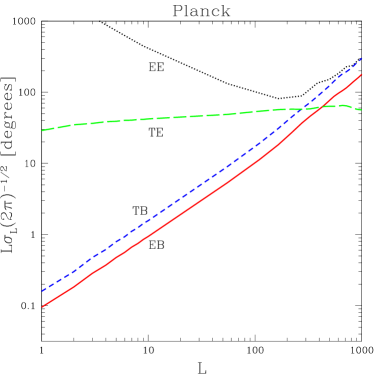
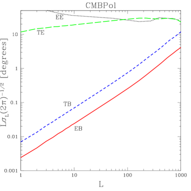
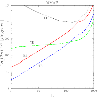
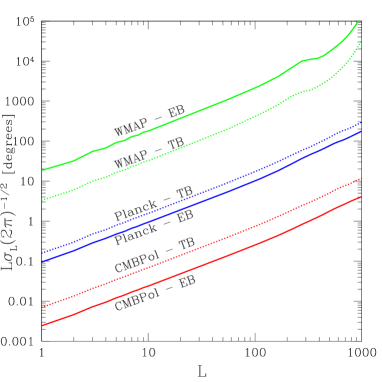
We evaluate the expressions for variances derived in the previous Section, for each of the three experiments, and show in Fig. 1 the numerical results for EB, EE, TB, and TE correlations.
Refer to caption
Refer to caption
Refer to caption
Figure 1: Variances for the four rotation estimators for WMAP, Planck, and CMBPol are shown. We see that, at low multipoles, the lowest-error estimator for Planck and CMBPol comes from the EB correlation, and for WMAP from the TB correlation.

The first thing to notice about the variance levels in these three experiments is that both the lower noise and the higher resolution contribute to about two orders of magnitude improvement in the sensitivity to a rotation from WMAP to Planck and will lead to yet more than another order-of-magnitude improvement in CMBPol. This is illustrated in more detail in Fig. 3, where the variances in the EB and TB estimators are compared for all three experiments.

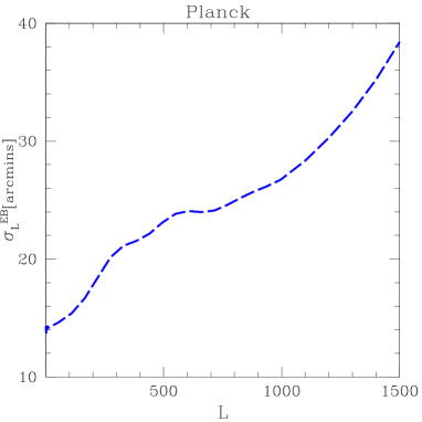
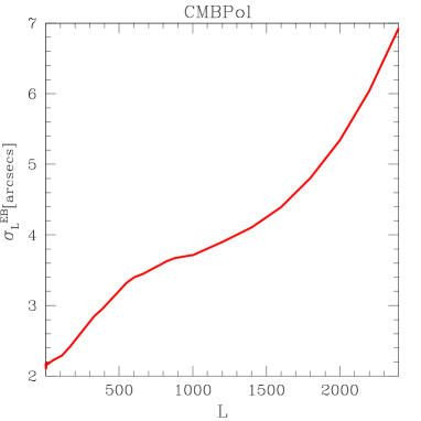
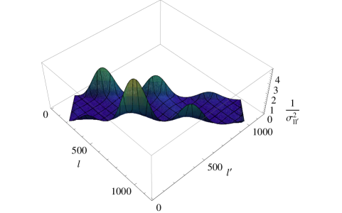
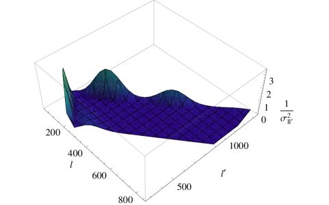
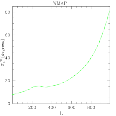
From Fig. 1, we see that, at low multipoles (below L𝐿L of about 200200200), the most sensitive estimators for all three experiments will be those derived from the EB and TB correlations. This comes about because of the absence of any TB or EB correlation under the assumption (justified largely by upper limits to the B mode amplitude) of no B modes at the surface of last scatter. We separately look at the TB-estimator variance for WMAP and the EB-estimator variances for Planck and CMBPol, in Fig. 2.
Refer to captionRefer to captionRefer to caption
Figure 2: The variances of the estimators for rotation are shown in linear scale, for WMAP (variance from the TB correlator), Planck (from EB) and CMBPol (from EB). The range of the plots is chosen so that it covers the resolution domain of the instrument. The exponential rise at high L𝐿L, due to the window function, is visible. Note the difference in scale on the y𝑦y-axis in all three panels.

For WMAP, we find a TB-estimator variance of 8.3superscript8.38.3^{\circ} at L=0𝐿0L=0, which is consistent with the current constraints on a uniform rotation101010Note that we calculate the multipole moments of rotation, so a uniform rotation of angle α𝛼\alpha has α00=4παsubscript𝛼004𝜋𝛼\alpha_{00}=\sqrt{4\pi}\alpha. Thus, α00=8.3subscript𝛼00superscript8.3\alpha_{00}=8.3^{\circ} is equivalent to α=2.3𝛼superscript2.3\alpha=2.3^{\circ}. Feng:2006dp ; Komatsu (see Appendix C). The dipole and quadrupole components of the rotation have the same variances as the monopole (L=0𝐿0L=0), since the variance remains fairly flat out to L𝐿L of about 100100100, in all three instruments. Above L400similar-to-or-equals𝐿400L\simeq 400, the variance increases rapidly. This happens when the exponential part of the window functions dominates (due to the finite angular resolution of the instrument). Also, since the correlation angle for polarization is about 101010 times smaller than that for temperature, the exponential tail in the EE-estimator case becomes prominent at higher multipoles than in the TE case. The variance from the EB-estimator at L=0𝐿0L=0 is 46.2superscript46.246.2^{\circ} for WMAP, and thus not constraining. The TE-estimator variance quickly drops below the EB-estimator variance (at L20similar-to-or-equals𝐿20L\simeq 20) and below the TB-estimator variance (at L150similar-to-or-equals𝐿150L\simeq 150). However, the variance σLsubscript𝜎𝐿\sigma_{L} at these L𝐿L is so large (100greater-than-or-equivalent-toabsent100\gtrsim 100) that the measurements are not at all constraining. Similar features are apparent in plots for the other two experiments.

For Planck, the variances of the EB and TB estimators are more comparable, and the constraints to all rotation multipoles in the range from L𝐿L of 00 to about 300300300 come from the EB variance. At L=0𝐿0L=0 the variance is 14superscript1414^{\prime} and 24superscript2424^{\prime}, for the EB- and TB-estimator variances, respectively. Planck can thus provide an order-of-magnitude better sensitivity to the uniform rotation than the current WMAP sensitivity. For high multipoles, above L400similar-to-or-equals𝐿400L\simeq 400 or so, the TE-estimator variance becomes the smallest one. At L800similar-to-or-equals𝐿800L\simeq 800, a rapid rise in all four variances is visible, due to the limitations in angular resolution and the correlation angle of the polarization.

For CMBPol, the EB-estimator variance is the smallest in the whole range of multipoles from 00 to 100010001000. At L=0𝐿0L=0, the EB and TB values are, respectively, 2.2"2.2"2.2" and 6.3"6.3"6.3", which is better than Planck by more than an order of magnitude. Similarly to WMAP and Planck variances, we observe a rapid rise in the variance above L1000similar-to-or-equals𝐿1000L\simeq 1000, corresponding to the resolution limitations and/or the polarization correlation length.
Refer to caption
Figure 3: The best constraints to rotation, i.e. the variances for estimators from the EB and TB correlations, are compared for three instruments. Planck gives about 2 orders of magnitude improvement in comparison to WMAP, and CMBPol is one order of magnitude better than Planck.

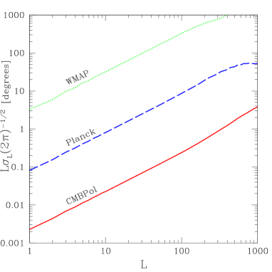
In Fig. 4 we show the variance for the combined minimum-variance estimator, obtained from all four estimators, with inverse-variance weighting. We have not included the covariance between the four estimators in this numerical calculation. However, this omission should make negligible difference for the WMAP and CMBPol curves, where the variance is determined primarily by TB and EB, respectively; the Planck curve may be increased, but only slightly. The run of this combined variance with L𝐿L differs very little from the smallest/constraining variance (that is TB in the case of WMAP and EB in the case of Planck and CMBPol), because that term dominates the sum.
Refer to caption
Figure 4: The combined variance, for all four estimators for rotation, is shown for WMAP, Planck and CMBPol. Note that, due to the inverse-weight summing, the smallest of the four variances dominates the shape of the curves.

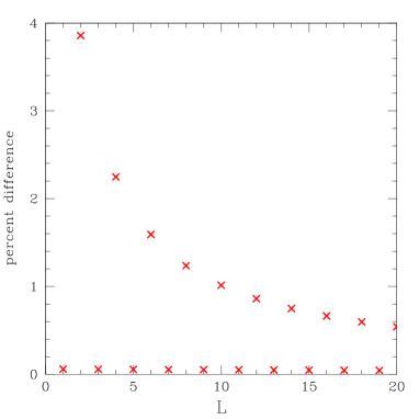
As a check, we repeated our calculations for the EB-correlator using the flat-sky formulas from §IV, and compared those results to the full-sky. The two sets of variances are in good agreement at high multipoles, where the flat sky makes a valid approximation (better than a fraction of a percent for L50greater-than-or-equivalent-to𝐿50L\gtrsim 50). The discrepancy increases up to 4%similar-toabsentpercent4\sim 4\% at lower L𝐿L. Fig. 5 compares the variances obtained from the full- and flat-sky treatments at low L𝐿L. Finally, we re-did the full-sky calculations using the same instrumental parameters as in Ref. Yadav:2009eb ; these are also in good agreement with our results at high L’s (better than 7%percent77\% for L50greater-than-or-equivalent-to𝐿50L\gtrsim 50, and about 11%percent1111\% at L=0𝐿0L=0).

Refer to caption
Figure 5: Comparison between the full- and flat-sky expressions for the variance in the low-L𝐿L regime. The discrepancy between the two is larger for even L𝐿L because of the additional contributions to the estimators from l=l𝑙superscript𝑙l=l^{\prime}.

VI Conclusions and Summary

Exotic mechanisms, such as quintessence fields that couple to the pseudoscalar of electromagnetism, could rotate the linear polarization of the CMB. In this paper, we derive the complete set of minimum-variance estimators for a position-dependent rotation of the CMB polarization, and thus provide a recipe, given a full-sky map, for measuring the rotation angle as a function of position on the sky. We also evaluate the variances with which the rotation-angle spherical-harmonic coefficients can be measured for WMAP, Planck, and CMBPol. Our results indicate that EB and TB correlations will provide more sensitive probes of the rotation angle than TE and EE correlations, and that EB becomes better, relative to TB, as the instrumental noise is reduced. We have checked that our results for the variances recover prior results, both analytically and numerically, in the flat-sky limit. As an additional check, Appendix C shows that our expressions for the rotation-angle variance recovers that expected for a uniform rotation. Appendix B shows that parity considerations can be used to distinguish the effects of rotation and of weak lensing on the CMB temperature/polarization map.

Now that we have elucidated the all-sky formalism, the next step will be to work out algorithms for recovery of the rotation angle for a map with partial sky coverage. We anticipate that analogous techniques for determining the cosmic-shear deflection angle may be adapted for this purpose.

Acknowledgements.
VG thanks Itamar Yaakov and Michael Kesden for useful comments. This work was supported by DoE DE-FG03-92-ER40701 and the Gordon and Betty Moore Foundation.

APPENDIX A: Some Useful Formulas

Some formulas used in §II and §III are included here. The metric tensor and its inverse on a unit 2-sphere (i.e. on the sky) is

g=(100sin2θ),𝑔10missing-subexpressionmissing-subexpressionmissing-subexpressionmissing-subexpressionmissing-subexpressionmissing-subexpressionmissing-subexpressionmissing-subexpressionmissing-subexpressionmissing-subexpressionmissing-subexpressionmissing-subexpressionmissing-subexpressionmissing-subexpressionmissing-subexpressionmissing-subexpressionmissing-subexpressionmissing-subexpression0superscript2𝜃missing-subexpressionmissing-subexpressionmissing-subexpressionmissing-subexpressionmissing-subexpressionmissing-subexpressionmissing-subexpressionmissing-subexpressionmissing-subexpressionmissing-subexpressionmissing-subexpressionmissing-subexpressionmissing-subexpressionmissing-subexpressionmissing-subexpressionmissing-subexpressionmissing-subexpressionmissing-subexpressiong=\left({\begin{array}[]{*{20}c}1&0\\ 0&{\sin^{2}\theta}\\ \end{array}}\right), (60)
g1=(1001sin2θ).superscript𝑔110missing-subexpressionmissing-subexpressionmissing-subexpressionmissing-subexpressionmissing-subexpressionmissing-subexpressionmissing-subexpressionmissing-subexpressionmissing-subexpressionmissing-subexpressionmissing-subexpressionmissing-subexpressionmissing-subexpressionmissing-subexpressionmissing-subexpressionmissing-subexpressionmissing-subexpressionmissing-subexpression01superscript2𝜃missing-subexpressionmissing-subexpressionmissing-subexpressionmissing-subexpressionmissing-subexpressionmissing-subexpressionmissing-subexpressionmissing-subexpressionmissing-subexpressionmissing-subexpressionmissing-subexpressionmissing-subexpressionmissing-subexpressionmissing-subexpressionmissing-subexpressionmissing-subexpressionmissing-subexpressionmissing-subexpressiong^{-1}=\left({\begin{array}[]{*{20}c}1&0\\ 0&{\frac{1}{{\sin^{2}\theta}}}\\ \end{array}}\right). (61)

The Levi-Civita tensor on a unit 2-sphere is

ε=(0sinθsinθ0).𝜀0𝜃missing-subexpressionmissing-subexpressionmissing-subexpressionmissing-subexpressionmissing-subexpressionmissing-subexpressionmissing-subexpressionmissing-subexpressionmissing-subexpressionmissing-subexpressionmissing-subexpressionmissing-subexpressionmissing-subexpressionmissing-subexpressionmissing-subexpressionmissing-subexpressionmissing-subexpressionmissing-subexpression𝜃0missing-subexpressionmissing-subexpressionmissing-subexpressionmissing-subexpressionmissing-subexpressionmissing-subexpressionmissing-subexpressionmissing-subexpressionmissing-subexpressionmissing-subexpressionmissing-subexpressionmissing-subexpressionmissing-subexpressionmissing-subexpressionmissing-subexpressionmissing-subexpressionmissing-subexpressionmissing-subexpression\varepsilon=\left({\begin{array}[]{*{20}c}0&{\sin\theta}\\ {-\sin\theta}&0\\ \end{array}}\right). (62)

An orthonormal basis on a unit 2-sphere is

e^θ=(10),e^ϕ=(0sinθ).formulae-sequencesubscript^𝑒𝜃10subscript^𝑒italic-ϕ0𝜃\hat{e}_{\theta}=\left(\begin{gathered}1\hfill\\ 0\hfill\\ \end{gathered}\right),\qquad\hat{e}_{\phi}=\left(\begin{gathered}0\hfill\\ \sin\theta\hfill\\ \end{gathered}\right). (63)

Some useful properties of the Wigner 3j symbols and related quantities include

(l1l2l3m1m2m3)=(1)l1+l2+l3(l1l2l3m1m2m3),subscript𝑙1subscript𝑙2subscript𝑙3missing-subexpressionmissing-subexpressionmissing-subexpressionmissing-subexpressionmissing-subexpressionmissing-subexpressionmissing-subexpressionmissing-subexpressionmissing-subexpressionmissing-subexpressionmissing-subexpressionmissing-subexpressionmissing-subexpressionmissing-subexpressionmissing-subexpressionmissing-subexpressionmissing-subexpressionsubscript𝑚1subscript𝑚2subscript𝑚3missing-subexpressionmissing-subexpressionmissing-subexpressionmissing-subexpressionmissing-subexpressionmissing-subexpressionmissing-subexpressionmissing-subexpressionmissing-subexpressionmissing-subexpressionmissing-subexpressionmissing-subexpressionmissing-subexpressionmissing-subexpressionmissing-subexpressionmissing-subexpressionmissing-subexpressionsuperscript1subscript𝑙1subscript𝑙2subscript𝑙3subscript𝑙1subscript𝑙2subscript𝑙3missing-subexpressionmissing-subexpressionmissing-subexpressionmissing-subexpressionmissing-subexpressionmissing-subexpressionmissing-subexpressionmissing-subexpressionmissing-subexpressionmissing-subexpressionmissing-subexpressionmissing-subexpressionmissing-subexpressionmissing-subexpressionmissing-subexpressionmissing-subexpressionmissing-subexpressionsubscript𝑚1subscript𝑚2subscript𝑚3missing-subexpressionmissing-subexpressionmissing-subexpressionmissing-subexpressionmissing-subexpressionmissing-subexpressionmissing-subexpressionmissing-subexpressionmissing-subexpressionmissing-subexpressionmissing-subexpressionmissing-subexpressionmissing-subexpressionmissing-subexpressionmissing-subexpressionmissing-subexpressionmissing-subexpression\left({\begin{array}[]{*{20}c}{l_{1}}&{l_{2}}&{l_{3}}\\ {m_{1}}&{m_{2}}&{m_{3}}\\ \end{array}}\right)=(-1)^{l_{1}+l_{2}+l_{3}}\left({\begin{array}[]{*{20}c}{l_{1}}&{l_{2}}&{l_{3}}\\ {-m_{1}}&{-m_{2}}&{-m_{3}}\\ \end{array}}\right), (64)
(l1l2l3m1m2m3)=(l2l3l1m2m3m1),subscript𝑙1subscript𝑙2subscript𝑙3missing-subexpressionmissing-subexpressionmissing-subexpressionmissing-subexpressionmissing-subexpressionmissing-subexpressionmissing-subexpressionmissing-subexpressionmissing-subexpressionmissing-subexpressionmissing-subexpressionmissing-subexpressionmissing-subexpressionmissing-subexpressionmissing-subexpressionmissing-subexpressionmissing-subexpressionsubscript𝑚1subscript𝑚2subscript𝑚3missing-subexpressionmissing-subexpressionmissing-subexpressionmissing-subexpressionmissing-subexpressionmissing-subexpressionmissing-subexpressionmissing-subexpressionmissing-subexpressionmissing-subexpressionmissing-subexpressionmissing-subexpressionmissing-subexpressionmissing-subexpressionmissing-subexpressionmissing-subexpressionmissing-subexpressionsubscript𝑙2subscript𝑙3subscript𝑙1missing-subexpressionmissing-subexpressionmissing-subexpressionmissing-subexpressionmissing-subexpressionmissing-subexpressionmissing-subexpressionmissing-subexpressionmissing-subexpressionmissing-subexpressionmissing-subexpressionmissing-subexpressionmissing-subexpressionmissing-subexpressionmissing-subexpressionmissing-subexpressionmissing-subexpressionsubscript𝑚2subscript𝑚3subscript𝑚1missing-subexpressionmissing-subexpressionmissing-subexpressionmissing-subexpressionmissing-subexpressionmissing-subexpressionmissing-subexpressionmissing-subexpressionmissing-subexpressionmissing-subexpressionmissing-subexpressionmissing-subexpressionmissing-subexpressionmissing-subexpressionmissing-subexpressionmissing-subexpressionmissing-subexpression\left({\begin{array}[]{*{20}{c}}{{l_{1}}}&{{l_{2}}}&{{l_{3}}}\\ {{m_{1}}}&{{m_{2}}}&{{m_{3}}}\\ \end{array}}\right)=\left({\begin{array}[]{*{20}{c}}{{l_{2}}}&{{l_{3}}}&{{l_{1}}}\\ {{m_{2}}}&{{m_{3}}}&{{m_{1}}}\\ \end{array}}\right), (65)
(l1l2l3m1m2m3)=(1)l1+l2+l3(l2l1l3m2m1m3),subscript𝑙1subscript𝑙2subscript𝑙3missing-subexpressionmissing-subexpressionmissing-subexpressionmissing-subexpressionmissing-subexpressionmissing-subexpressionmissing-subexpressionmissing-subexpressionmissing-subexpressionmissing-subexpressionmissing-subexpressionmissing-subexpressionmissing-subexpressionmissing-subexpressionmissing-subexpressionmissing-subexpressionmissing-subexpressionsubscript𝑚1subscript𝑚2subscript𝑚3missing-subexpressionmissing-subexpressionmissing-subexpressionmissing-subexpressionmissing-subexpressionmissing-subexpressionmissing-subexpressionmissing-subexpressionmissing-subexpressionmissing-subexpressionmissing-subexpressionmissing-subexpressionmissing-subexpressionmissing-subexpressionmissing-subexpressionmissing-subexpressionmissing-subexpressionsuperscript1subscript𝑙1subscript𝑙2subscript𝑙3subscript𝑙2subscript𝑙1subscript𝑙3missing-subexpressionmissing-subexpressionmissing-subexpressionmissing-subexpressionmissing-subexpressionmissing-subexpressionmissing-subexpressionmissing-subexpressionmissing-subexpressionmissing-subexpressionmissing-subexpressionmissing-subexpressionmissing-subexpressionmissing-subexpressionmissing-subexpressionmissing-subexpressionmissing-subexpressionsubscript𝑚2subscript𝑚1subscript𝑚3missing-subexpressionmissing-subexpressionmissing-subexpressionmissing-subexpressionmissing-subexpressionmissing-subexpressionmissing-subexpressionmissing-subexpressionmissing-subexpressionmissing-subexpressionmissing-subexpressionmissing-subexpressionmissing-subexpressionmissing-subexpressionmissing-subexpressionmissing-subexpressionmissing-subexpression\left({\begin{array}[]{*{20}{c}}{{l_{1}}}&{{l_{2}}}&{{l_{3}}}\\ {{m_{1}}}&{{m_{2}}}&{{m_{3}}}\\ \end{array}}\right)={(-1)^{{l_{1}}+{l_{2}}+{l_{3}}}}\left({\begin{array}[]{*{20}{c}}{{l_{2}}}&{{l_{1}}}&{{l_{3}}}\\ {{m_{2}}}&{{m_{1}}}&{{m_{3}}}\\ \end{array}}\right), (66)
(ll0mm0)=(1)lm2l+1,𝑙𝑙0missing-subexpressionmissing-subexpressionmissing-subexpressionmissing-subexpressionmissing-subexpressionmissing-subexpressionmissing-subexpressionmissing-subexpressionmissing-subexpressionmissing-subexpressionmissing-subexpressionmissing-subexpressionmissing-subexpressionmissing-subexpressionmissing-subexpressionmissing-subexpressionmissing-subexpression𝑚𝑚0missing-subexpressionmissing-subexpressionmissing-subexpressionmissing-subexpressionmissing-subexpressionmissing-subexpressionmissing-subexpressionmissing-subexpressionmissing-subexpressionmissing-subexpressionmissing-subexpressionmissing-subexpressionmissing-subexpressionmissing-subexpressionmissing-subexpressionmissing-subexpressionmissing-subexpressionsuperscript1𝑙𝑚2𝑙1\left({\begin{array}[]{*{20}{c}}l&l&0\\ m&{-m}&0\\ \end{array}}\right)=\frac{{{{(-1)}^{l-m}}}}{{\sqrt{2l+1}}}, (67)
m1+m2+m30(l1l2l3m1m2m3)=0,subscript𝑚1subscript𝑚2subscript𝑚30subscript𝑙1subscript𝑙2subscript𝑙3missing-subexpressionmissing-subexpressionmissing-subexpressionmissing-subexpressionmissing-subexpressionmissing-subexpressionmissing-subexpressionmissing-subexpressionmissing-subexpressionmissing-subexpressionmissing-subexpressionmissing-subexpressionmissing-subexpressionmissing-subexpressionmissing-subexpressionmissing-subexpressionmissing-subexpressionsubscript𝑚1subscript𝑚2subscript𝑚3missing-subexpressionmissing-subexpressionmissing-subexpressionmissing-subexpressionmissing-subexpressionmissing-subexpressionmissing-subexpressionmissing-subexpressionmissing-subexpressionmissing-subexpressionmissing-subexpressionmissing-subexpressionmissing-subexpressionmissing-subexpressionmissing-subexpressionmissing-subexpressionmissing-subexpression0m_{1}+m_{2}+m_{3}\neq 0\Rightarrow\left({\begin{array}[]{*{20}c}l_{1}&l_{2}&{l_{3}}\\ m_{1}&m_{2}&m_{3}\\ \end{array}}\right)=0, (68)
m1m2(2l3+1)(l1l2l3m1m2m3)(l1l2l3m1m2m3)=δl3l3δm3m3.subscriptsubscript𝑚1subscript𝑚22subscript𝑙31subscript𝑙1subscript𝑙2subscript𝑙3missing-subexpressionmissing-subexpressionmissing-subexpressionmissing-subexpressionmissing-subexpressionmissing-subexpressionmissing-subexpressionmissing-subexpressionmissing-subexpressionmissing-subexpressionmissing-subexpressionmissing-subexpressionmissing-subexpressionmissing-subexpressionmissing-subexpressionmissing-subexpressionmissing-subexpressionsubscript𝑚1subscript𝑚2subscript𝑚3missing-subexpressionmissing-subexpressionmissing-subexpressionmissing-subexpressionmissing-subexpressionmissing-subexpressionmissing-subexpressionmissing-subexpressionmissing-subexpressionmissing-subexpressionmissing-subexpressionmissing-subexpressionmissing-subexpressionmissing-subexpressionmissing-subexpressionmissing-subexpressionmissing-subexpressionsubscript𝑙1subscript𝑙2superscriptsubscript𝑙3missing-subexpressionmissing-subexpressionmissing-subexpressionmissing-subexpressionmissing-subexpressionmissing-subexpressionmissing-subexpressionmissing-subexpressionmissing-subexpressionmissing-subexpressionmissing-subexpressionmissing-subexpressionmissing-subexpressionmissing-subexpressionmissing-subexpressionmissing-subexpressionmissing-subexpressionsubscript𝑚1subscript𝑚2superscriptsubscript𝑚3missing-subexpressionmissing-subexpressionmissing-subexpressionmissing-subexpressionmissing-subexpressionmissing-subexpressionmissing-subexpressionmissing-subexpressionmissing-subexpressionmissing-subexpressionmissing-subexpressionmissing-subexpressionmissing-subexpressionmissing-subexpressionmissing-subexpressionmissing-subexpressionmissing-subexpressionsubscript𝛿subscript𝑙3superscriptsubscript𝑙3subscript𝛿subscript𝑚3superscriptsubscript𝑚3\begin{gathered}\sum\limits_{{m_{1}}{m_{2}}}{}(2{l_{3}}+1)\left({\begin{array}[]{*{20}{c}}{{l_{1}}}&{{l_{2}}}&{{l_{3}}}\\ {{m_{1}}}&{{m_{2}}}&{{m_{3}}}\\ \end{array}}\right)\left(\begin{array}[]{*{20}{c}}{{l_{1}}}&{{l_{2}}}&{{l_{3}}^{\prime}}\\ {{m_{1}}}&{{m_{2}}}&{{m_{3}}^{\prime}}\\ \end{array}\right)\hfill\\ ={\delta_{{l_{3}}{l_{3}}^{\prime}}}{\delta_{{m_{3}}{m_{3}}^{\prime}}}.\end{gathered} (69)

The relation between spherical harmonics and Wigner 3j symbols is

𝑑n^Yl1m1(𝐧^)Yl2m2(𝐧^)Yl3m3(𝐧^)=(2l1+1)(2l2+1)(2l3+1)4π×(l1l2l3m1m2m3)(l1l2l3000)differential-d^𝑛subscript𝑌subscript𝑙1subscript𝑚1^𝐧subscript𝑌subscript𝑙2subscript𝑚2^𝐧subscript𝑌subscript𝑙3subscript𝑚3^𝐧2subscript𝑙112subscript𝑙212subscript𝑙314𝜋subscript𝑙1subscript𝑙2subscript𝑙3missing-subexpressionmissing-subexpressionmissing-subexpressionmissing-subexpressionmissing-subexpressionmissing-subexpressionmissing-subexpressionmissing-subexpressionmissing-subexpressionmissing-subexpressionmissing-subexpressionmissing-subexpressionmissing-subexpressionmissing-subexpressionmissing-subexpressionmissing-subexpressionmissing-subexpressionsubscript𝑚1subscript𝑚2subscript𝑚3missing-subexpressionmissing-subexpressionmissing-subexpressionmissing-subexpressionmissing-subexpressionmissing-subexpressionmissing-subexpressionmissing-subexpressionmissing-subexpressionmissing-subexpressionmissing-subexpressionmissing-subexpressionmissing-subexpressionmissing-subexpressionmissing-subexpressionmissing-subexpressionmissing-subexpressionsubscript𝑙1subscript𝑙2subscript𝑙3missing-subexpressionmissing-subexpressionmissing-subexpressionmissing-subexpressionmissing-subexpressionmissing-subexpressionmissing-subexpressionmissing-subexpressionmissing-subexpressionmissing-subexpressionmissing-subexpressionmissing-subexpressionmissing-subexpressionmissing-subexpressionmissing-subexpressionmissing-subexpressionmissing-subexpression000missing-subexpressionmissing-subexpressionmissing-subexpressionmissing-subexpressionmissing-subexpressionmissing-subexpressionmissing-subexpressionmissing-subexpressionmissing-subexpressionmissing-subexpressionmissing-subexpressionmissing-subexpressionmissing-subexpressionmissing-subexpressionmissing-subexpressionmissing-subexpressionmissing-subexpression\begin{gathered}\int{d\hat{n}{Y_{{l_{1}}{m_{1}}}(\mathbf{\hat{n}})}{Y_{{l_{2}}{m_{2}}}(\mathbf{\hat{n}})}{Y_{{l_{3}}{m_{3}}}(\mathbf{\hat{n}})}}\\ =\sqrt{\frac{{(2{l_{1}}+1)(2{l_{2}}+1)(2{l_{3}}+1)}}{{4\pi}}}\\ \times\left({\begin{array}[]{*{20}{c}}{{l_{1}}}&{{l_{2}}}&{{l_{3}}}\\ {{m_{1}}}&{{m_{2}}}&{{m_{3}}}\\ \end{array}}\right)\left({\begin{array}[]{*{20}{c}}{{l_{1}}}&{{l_{2}}}&{{l_{3}}}\\ 0&0&0\\ \end{array}}\right)\end{gathered} (70)

APPENDIX B: Rotation vs. Weak Lensing

The effects of rotation and weak lensing Hu:2000ee ; lensing on polarization are orthogonal and can thus be distinguished geometrically with a full-sky map. For example, if we start off with a pure E mode at the surface of last scatter, rotation induces a B mode, given by Eq. (6), where the only non-zero terms are those that satisfy L+l+l2=𝐿𝑙subscript𝑙2absentL+l+l_{2}=even. However, if we analyse the effect of weak lensing (see Ref. lensing ), a pure E mode polarization tensor changes by

δPab=(cφ)(cPab),𝛿subscript𝑃𝑎𝑏subscript𝑐𝜑superscript𝑐subscript𝑃𝑎𝑏\delta{P_{ab}}=({\nabla_{c}}\varphi)({\nabla^{c}}{P_{ab}}), (71)

where φ𝜑\varphi is the projection of the gravitational potential along the line of sight. Thus, the B mode induced by weak lensing is

δBlm=𝑑n^δPab(n^)Y(lm)B,ab(n^)=2LMl2m2φLMEl2m2𝑑n^Y(lm)B,ab(cY(LM))(cY(l2m2)abE).𝛿subscript𝐵𝑙𝑚differential-d^𝑛𝛿subscript𝑃𝑎𝑏^𝑛subscriptsuperscript𝑌𝐵𝑎𝑏𝑙𝑚^𝑛2subscript𝐿𝑀subscriptsubscript𝑙2subscript𝑚2subscript𝜑𝐿𝑀subscript𝐸subscript𝑙2subscript𝑚2differential-d^𝑛subscriptsuperscript𝑌𝐵𝑎𝑏𝑙𝑚subscript𝑐subscript𝑌𝐿𝑀superscript𝑐subscriptsuperscript𝑌𝐸subscript𝑙2subscript𝑚2𝑎𝑏\begin{gathered}\delta B_{lm}=\int{d\hat{n}\delta P_{ab}(\hat{n})Y^{B*,ab}_{(lm)}}(\hat{n})\hfill\\ =2\sum\limits_{LM}{\sum\limits_{l_{2}m_{2}}}\varphi_{LM}E_{l_{2}m_{2}}\hfill\\ \int{d\hat{n}}Y^{B*,ab}_{(lm)}(\nabla_{c}Y_{(LM)})(\nabla^{c}Y^{E}_{(l_{2}m_{2})ab}).\end{gathered} (72)

The parity of the spherical harmonic YLMsubscript𝑌𝐿𝑀Y_{LM} is (1)Lsuperscript1𝐿(-1)^{L}. The parity of the E-mode term in the integral is (1)l2superscript1subscript𝑙2(-1)^{l_{2}}, and the parity of the B-mode term is (1)l+1superscript1𝑙1(-1)^{l+1}. The parity of the integrand in Eq. (72) is then (1)L+l+l2+1superscript1𝐿𝑙subscript𝑙21(-1)^{L+l+l_{2}+1}. Therefore, the integral is non-vanishing only for terms that satisfy L+l+l2=𝐿𝑙subscript𝑙2absentL+l+l_{2}=odd.

We conclude that the rotation induces B modes that satisfy L+l+l2=𝐿𝑙subscript𝑙2absentL+l+l_{2}=even, while for weak lensing we have L+l+l2=𝐿𝑙subscript𝑙2absentL+l+l_{2}=odd [see Eqs. (6) and (20)]. Thus, the two effects can be entirely separated.

Strictly speaking, this orthogonality between lensing and rotation occurs only at linear order in the rotation and lensing amplitudes in the limit that lensing and rotation are both small. If a lensed field is then rotated, and/or if a rotated field is then lensed, then the orthogonality will break down. However, this will occur only with an amplitude that is proportional to the product of the lensing and rotation amplitudes. We have here implicitly assumed this to be small and leave the full treatment of this higher-order effect for future work.

APPENDIX C: Uniform Rotation Cross-Check

We can perform a cross-check of our formulas for variances of the rotation, by analyzing only the L=0𝐿0L=0 term, where all the representation-theory coefficients can be readily evaluated. We do so for the EB case. From Eqs. (49) and (50) (for l=l𝑙superscript𝑙l=l^{\prime}), after evaluating the coefficients for L=0𝐿0L=0, we get the variance of the uniform-rotation estimator to be

(σ00)2=1πl[ClEE(Wl)2]2(2l+1)ClEE,mapClBB,map.superscriptsubscript𝜎0021𝜋subscript𝑙superscriptdelimited-[]superscriptsubscript𝐶𝑙𝐸𝐸superscriptsubscript𝑊𝑙222𝑙1superscriptsubscript𝐶𝑙𝐸𝐸,mapsuperscriptsubscript𝐶𝑙𝐵𝐵,map{\begin{gathered}{(\sigma_{00})^{-2}}=\frac{1}{\pi}\sum\limits_{l}{\frac{{{[C_{l}^{EE}{{({W_{l}})}^{2}}]}^{2}(2l+1)}}{C_{l}^{EE\text{,map}}C_{l}^{BB\text{,map}}}}\hfill\\ \end{gathered}}. (73)

We can see that this is indeed the right expression for uniform rotation, by noting that the B mode induced by small rotation, from a pure E mode, is given by Eq. (3). The induced EB power spectrum in that case is

ClEB=2αClEE,superscriptsubscript𝐶𝑙𝐸𝐵2𝛼superscriptsubscript𝐶𝑙𝐸𝐸C_{l}^{EB}=2{\alpha}C_{l}^{EE}, (74)

and estimators for the rotation can be expressed for each lm𝑙𝑚lm pair as

α^=ElmmapBlmmap2ClEEWl2.^𝛼superscriptsubscript𝐸𝑙𝑚mapsuperscriptsubscript𝐵𝑙𝑚map2superscriptsubscript𝐶𝑙𝐸𝐸superscriptsubscript𝑊𝑙2{{\hat{\alpha}}}=\frac{{E_{lm}^{\text{map}}B_{lm}^{\text{map}}}}{{2C_{l}^{EE}W_{l}^{2}}}. (75)

The variance of rotation is then calculated from all lm𝑙𝑚lm pairs as

σ2=l=0m=ll1(α^)2=l(2l+1)4[ClEE(Wl)2]2ClEE,mapClBB,map,superscript𝜎2superscriptsubscript𝑙0superscriptsubscript𝑚𝑙𝑙1delimited-⟨⟩superscript^𝛼2subscript𝑙2𝑙14superscriptdelimited-[]superscriptsubscript𝐶𝑙𝐸𝐸superscriptsubscript𝑊𝑙22superscriptsubscript𝐶𝑙𝐸𝐸,mapsuperscriptsubscript𝐶𝑙𝐵𝐵,map\begin{gathered}\sigma^{-2}=\sum\limits_{l=0}^{\infty}{\sum\limits_{m=-l}^{l}{}}\frac{1}{{\left\langle{{{({{\hat{\alpha}}})}^{2}}}\right\rangle}}=\sum\limits_{l}(2l+1)\frac{{4{{[C_{l}^{EE}{{({W_{l}})}^{2}}]}^{2}}}}{{C_{l}^{EE{\text{,map}}}C_{l}^{BB{\text{,map}}}}},\end{gathered} (76)

where the factor of (2l+1)2𝑙1(2l+1) comes from the sum over m𝑚m, because the terms in the sum have effectively only index l𝑙l. For L=0𝐿0L=0, Eq. (76) reduces to Eq. (73), once the factor of 4π4𝜋\sqrt{4\pi} by which α𝛼\alpha and α00subscript𝛼00\alpha_{00} differ is taken into account.

APPENDIX D: Contributions of Multipole pairs to Rotation Estimator
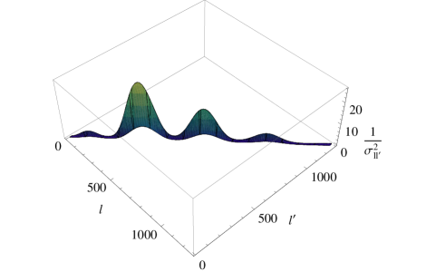
Refer to captionRefer to captionRefer to caption
Figure 6: The summands in Eq. (47) are plotted versus l𝑙l and lsuperscript𝑙l^{\prime}. Plots for three different rotation multipole coefficients are shown: L=20𝐿20L=20 (top panel), L=200𝐿200L=200 (middle panel), and L=500𝐿500L=500 (bottom panel). The plots suggest that the major contribution to any given rotation multipole coefficient comes from the ll𝑙superscript𝑙ll^{\prime} estimators that correspond to the strongest peaks in the EE power spectrum above the resolution limit of the instrument.
Refer to caption
Figure 7: The EE power spectrum used for numerical estimates in §V is shown. The main peaks of the power spectrum are visible at L150similar-to𝐿150L\sim 150, 400400400, 700700700, and 700700700.

In Fig. 6, we show the summand in Eq. (47), versus l𝑙l and lsuperscript𝑙l^{\prime}, for L=20𝐿20L=20, 200200200, and 500500500. These terms are the weights with which each ll𝑙superscript𝑙ll^{\prime} pair contributes to the EB estimator α^LMsubscript^𝛼𝐿𝑀\hat{\alpha}_{LM} for Planck (see Eq. (46)). Fig. 6 therefore illustrates which multipoles in the EE power spectrum are expected to contribute most to the three chosen rotation multipoles. From the Figure, we see that the region allowed by triangle inequalities grows with L𝐿L, and that the peaks along lsuperscript𝑙l^{\prime} correspond to the peaks in the EE power spectrum. There is also an overall exponential decay from the window functions, with a characteristic scale of l1000similar-tosuperscript𝑙1000l^{\prime}\sim 1000, beyond which the distributions fall to zero.

Overall, the EE multipoles that affect the estimate of the rotation at L=20𝐿20L=20 and 200200200 seem to be predominantly those that correspond to the strongest peaks in the EE power spectrum, below the resolution limit of l1000similar-tosuperscript𝑙1000l^{\prime}\sim 1000 (i.e. lsuperscript𝑙l^{\prime} of about 400400400, 700700700, and 100010001000; see Fig. 7). The relative contributions are shown in the top two panels of Fig. 6. The bottom panel of the same Figure shows the L=500𝐿500L=500 case. There, we see that the largest contribution is local, i.e. it comes from non-flat triangles at multipoles below l500similar-tosuperscript𝑙500l^{\prime}\sim 500, and the secondary contribution comes from the EE power-spectrum peaks at lsuperscript𝑙l^{\prime} of about 700700700 and 100010001000 (see Fig. 7).

References

  • (1) P. de Bernardis et al. [Boomerang Collaboration], Nature 404, 955 (2000) [arXiv:astro-ph/0004404]; A. D. Miller et al., Astrophys. J.  524, L1 (1999) [arXiv:astro-ph/9906421]; S. Hanany et al., Astrophys. J.  545, L5 (2000) [arXiv:astro-ph/0005123]; N. W. Halverson et al., Astrophys. J.  568, 38 (2002) [arXiv:astro-ph/0104489]; B. S. Mason et al., Astrophys. J.  591, 540 (2003) [arXiv:astro-ph/0205384]; A. Benoit et al. [the Archeops Collaboration], Astron. Astrophys.  399, L25 (2003) [arXiv:astro-ph/0210306]; J. H. Goldstein et al., Astrophys. J.  599, 773 (2003) [arXiv:astro-ph/0212517]; D. N. Spergel et al. [WMAP Collaboration], Astrophys. J. Suppl.  148, 175 (2003) [arXiv:astro-ph/0302209]; C. L. Reichardt et al., arXiv:0801.1491 [astro-ph]; D. N. Spergel et al. [WMAP Collaboration], Astrophys. J. Suppl.  170, 377 (2007) [arXiv:astro-ph/0603449]; J. Dunkley et al. [WMAP Collaboration], Astrophys. J. Suppl.  180, 306 (2009) [arXiv:0803.0586 [astro-ph]].
  • (2) J. Bock et al., arXiv:astro-ph/0604101.
  • (3) A. H. Guth, Phys. Rev.  D 23, 347 (1981); A. Albrecht and P. J. Steinhardt, Phys. Rev. Lett.  48, 1220 (1982); A. D. Linde, Phys. Lett.  B 108, 389 (1982).
  • (4) M. Kamionkowski and A. Kosowsky, Ann. Rev. Nucl. Part. Sci.  49, 77 (1999) [arXiv:astro-ph/9904108].
  • (5) M. Kamionkowski, A. Kosowsky and A. Stebbins, Phys. Rev.  D 55, 7368 (1997) [arXiv:astro-ph/9611125]; M. Kamionkowski, A. Kosowsky and A. Stebbins, Phys. Rev. Lett.  78, 2058 (1997) [arXiv:astro-ph/9609132].
  • (6) M. Zaldarriaga and U. Seljak, Phys. Rev.  D 55, 1830 (1997) [arXiv:astro-ph/9609170]. U. Seljak and M. Zaldarriaga, Phys. Rev. Lett.  78, 2054 (1997) [arXiv:astro-ph/9609169].
  • (7) M. Kamionkowski and A. Kosowsky, Phys. Rev.  D 57, 685 (1998) [arXiv:astro-ph/9705219].
  • (8) S. M. Carroll, Phys. Rev. Lett.  81, 3067 (1998) [arXiv:astro-ph/9806099].
  • (9) A. Lue, L. M. Wang and M. Kamionkowski, Phys. Rev. Lett.  83, 1506 (1999) [arXiv:astro-ph/9812088]; N. F. Lepora, arXiv:gr-qc/9812077; K. R. S. Balaji, R. H. Brandenberger and D. A. Easson, JCAP 0312, 008 (2003) [arXiv:hep-ph/0310368].
  • (10) B. Feng et al., Phys. Rev. Lett.  96, 221302 (2006) [arXiv:astro-ph/0601095]; T. Kahniashvili, R. Durrer and Y. Maravin, arXiv:0807.2593 [astro-ph]; J. Q. Xia et al., arXiv:0803.2350 [astro-ph]; J. Q. Xia et al., arXiv:0710.3325 [hep-ph]; :. E. Y. Wu et al. [QUaD Collaboration], arXiv:0811.0618 [astro-ph]; L. Pagano et al., arXiv:0905.1651 [astro-ph.CO].
  • (11) E. Komatsu et al. [WMAP Collaboration], arXiv:0803.0547 [astro-ph].
  • (12) M. Pospelov, A. Ritz and C. Skordis, arXiv:0808.0673 [astro-ph]; M. Li and X. Zhang, Phys. Rev.  D 78, 103516 (2008) [arXiv:0810.0403 [astro-ph]].
  • (13) S. Gardner, Phys. Rev. Lett.  100, 041303 (2008) [arXiv:astro-ph/0611684].
  • (14) M. Kamionkowski, arXiv:0810.1286 [astro-ph].
  • (15) A. P. S. Yadav, R. Biswas, M. Su and M. Zaldarriaga, arXiv:0902.4466 [astro-ph.CO].
  • (16) http://www.rssd.esa.int/PLANCK.
  • (17) J. Bock et al., arXiv:0805.4207 [astro-ph].
  • (18) A. L. Erickcek, S. M. Carroll and M. Kamionkowski, Phys. Rev.  D 78, 083012 (2008) [arXiv:0808.1570 [astro-ph]]; A. L. Erickcek, M. Kamionkowski and S. M. Carroll, Phys. Rev.  D 78, 123520 (2008) [arXiv:0806.0377 [astro-ph]].
  • (19) A. R. Pullen and M. Kamionkowski, Phys. Rev.  D 76, 103529 (2007) [arXiv:0709.1144 [astro-ph]].
  • (20) J. Hoftuft et al., arXiv:0903.1229 [astro-ph.CO]; F. K. Hansen et al., arXiv:0812.3795 [astro-ph]; H. K. Eriksen et al., Astrophys. J.  605, 14 (2004) [Erratum-ibid.  609, 1198 (2004)] [arXiv:astro-ph/0307507]; F. K. Hansen, A. J. Banday, and K. M. Górski, Mon. Not. Roy. Astron. Soc.  354, 641 (2004) [arXiv:astro-ph/040420]; H. K. Eriksen et al., Astrophys. J.  660, L81 (2007) [arXiv:astro-ph/0701089].
  • (21) W. Hu, Phys. Rev.  D 62, 043007 (2000) [arXiv:astro-ph/0001303].
  • (22) A. Hajian and T. Souradeep, arXiv:astro-ph/0501001; T. Souradeep, A. Hajian and S. Basak, New Astron. Rev.  50, 889 (2006) [arXiv:astro-ph/0607577]; A. Hajian and T. Souradeep, Phys. Rev.  D 74, 123521 (2006) [arXiv:astro-ph/0607153]; A. Hajian and T. Souradeep, Astrophys. J.  597, L5 (2003) [arXiv:astro-ph/0308001]; S. Basak, A. Hajian and T. Souradeep, Phys. Rev.  D 74, 021301 (2006) [arXiv:astro-ph/0603406].
  • (23) M. Betoule et al., arXiv:0901.1056 [astro-ph.CO].
  • (24) M. Zaldarriaga and U. Seljak, Phys. Rev.  D 58, 023003 (1998) [arXiv:astro-ph/9803150]; U. Seljak and M. Zaldarriaga, Phys. Rev. Lett.  82, 2636 (1999) [arXiv:astro-ph/9810092]; M. Zaldarriaga and U. Seljak, Phys. Rev.  D 59, 123507 (1999) [arXiv:astro-ph/9810257]; T. Okamoto and W. Hu, Phys. Rev.  D 67, 083002 (2003) [arXiv:astro-ph/0301031]; W. Hu and T. Okamoto, Astrophys. J.  574, 566 (2002) [arXiv:astro-ph/0111606]; M. Kesden, A. Cooray and M. Kamionkowski, Phys. Rev. Lett.  89, 011304 (2002) [arXiv:astro-ph/0202434]; L. Knox and Y. S. Song, Phys. Rev. Lett.  89, 011303 (2002) [arXiv:astro-ph/0202286]; M. H. Kesden, A. Cooray and M. Kamionkowski, Phys. Rev.  D 67, 123507 (2003) [arXiv:astro-ph/0302536]; P. Cabella and M. Kamionkowski, arXiv:astro-ph/0403392; A. Lewis and A. Challinor, Phys. Rept.  429, 1 (2006) [arXiv:astro-ph/0601594].