Nonlinear preferential rewiring in fixed-size networks as a diffusion process

Abstract

We present an evolving network model in which the total numbers of nodes and edges are conserved, but in which edges are continuously rewired according to nonlinear preferential detachment and reattachment. Assuming power-law kernels with exponents $\alpha$ and $\beta$, the stationary states the degree distributions evolve towards exhibit a second order phase transition – from relatively homogeneous to highly heterogeneous (with the emergence of starlike structures) at $\alpha=\beta$. Temporal evolution of the distribution in this critical regime is shown to follow a nonlinear diffusion equation, arriving at either pure or mixed power-laws, of exponents $-\alpha$ and $1-\alpha$.

Complex systems may often be described as a set of nodes with edges connecting some of them – the neighbours – (see, for instance, Refs.gen ; gen1 ; gen2 ). The number of edges a particular node has is called its degree, $k$. The study of such large networks is usually made simpler by considering statistical properties, e.g., the degree distribution, $p(k)$ (probability of finding a node with a particular degree). It turns out that a high proportion of real-world networks follow power-law degree distributions, $p(k)\sim k^{-\gamma}$ – referred to as scale-free due to their lack of a characteristic size. Also, many of them have their edges placed among the nodes apparently in a random way – i.e., there is no correlation between the degree of a node and any other of its properties, such as the degrees of its neighbours. Barabási and Albert Barabasi applied the mechanism of preferential attachment to an evolving network model and showed how this resulted in the degree distributions becoming scale-free for long enough times. For this to work, attachment had to be linear – i.e., the probability a node with degree $k$ has of receiving a new edge is $\pi(k)\sim k+q$. This results in scale-free stationary degree distributions with an exponent $\gamma=3-q$.

Preferential attachment seems to be behind the emergence of many real-world, continuously growing networks. However, not all networks in which some nodes at times gain (or loose) new edges have a continuously growing number of nodes. For example, a given group of people may form an evolving social network Kossinets in which the edges represent friendship. Preferential attachment may be relevant here – the more people you know, the more likely it is that you will be introduced to someone new – but probabilities are not expected to depend linearly on degree. For instance, there may be saturations (highly connected people might become less accessible), threshold effects (hermits may be prone to antisocial tendencies), and other non-linearities. The brain may also be a relevant case. Once formed, the number of neurons does not seem to continually augment, and yet its structural topology is dynamic Klintsova . Synaptic growth and dendritic arborization have been shown to increase with electric stimulation Lee ; DeRoo – and, in general, the more connected a neuron is, the more current it receives from the sum of its neighbours.

Barabási and Albert showed that both (linear) preferential attachment and an ever-growing number of nodes are needed for scaling to emerge in their model. In a fixed population, their mechanism would result in a fully-connected network. However, this is not normally observed in real systems. Rather, just as some new edges sprout, others disappear – less used synapses suffer atrophy, unstimulating friendships wither. Often, the numbers of both nodes and edges remain roughly constant. The same authors did therefore extend their model so as to include the effects of preferential rewiring (which could be applied to fixed-size networks), although again probabilities depended linearly on node degree Albert . Another mechanism which (roughly) maintains constant the numbers of nodes and edges is node fusing Thurner , once more according to linear probabilities. As to nonlinear preferential attachment, the (growing) BA model was extended to take power-law probabilities into account Krapivsky , although the solutions are only scale free for the linear case.

In this note we present an evolving network model with preferential rewiring according to nonlinear (power-law) probabilities. The number of nodes and edges is conserved but the topology evolves, arriving eventually at a macroscopically (nonequilibrium) stationary state – as described by global properties such as the degree distribution. Depending on the exponents chosen for the rewiring probabilities, the final state can be either fairly homogeneous, with a typical size, or highly heterogeneous, with the emergence of starlike structures. In the critical case marking the transition between these two regimes, the degree distribution is shown to follow a nonlinear diffusion equation. This describes a tendency towards stationary states that are characterized either by scale-free or by mixed scale-free distributions, depending on parameters.

Our model consists of a random network with $N$ nodes of respective degree $k_{i},$ $i=1,2,...,N,$ and $\frac{1}{2}N\left\langle k\right\rangle$ edges. Initially, the degrees have a given distribution $p(k,t=0)$. At each time step, one node is chosen with a probability which is a function of its degree, $\rho(k_{i})$. One of its edges is then chosen randomly and removed from it, to be reconnected to another node $j$ chosen according to a probability $\pi(k_{j})$. That is, an edge is broken and another one is created, and the total number of edges, as well as the total number of nodes, is conserved. The functions $\pi(k)$ and $\rho(k)$ are arbitrary, but we shall explicitly illustrate here $\pi(k_{i})\sim k_{i}^{\alpha}$ and $\rho(k_{i})\sim k_{i}^{\beta}$ that capture the essence of a wide class of nonlinear monotonous response functions and are easy to handle analytically.

The probabilities $\pi$ and $\rho$ a given node has, at each time step, of increasing or decreasing its degree can be interpreted as transition probabilities between states. The expected value of the increment in a given $p(k,t)$ at each time step, $\Delta p(k,t)$, may then be written as

$$\frac{\partial p(k,t)}{\partial t} =(k-1)^{\alpha}\,\bar{k}_{\alpha}^{-1}p(k-1,t)$$

$$+(k+1)^{\beta}\,\bar{k}_{\beta}^{-1}\,p(k+1,t)$$ (1)

$$-\left(k^{\alpha}\,\bar{k}_{\alpha}^{-1}+k^{\beta}\,\bar{k}_{\beta}^{-1}\right)\,p(k,t),$$

where $\bar{k}_{a}=\bar{k}_{a}\left(t\right)=\sum_{k}k^{a}p(k,t).$ If it exists, any stationary solution must satisfy the condition $p_{\text{st}}(k+1)\,(k+1)^{\beta}\,\bar{k}_{\alpha}^{\text{st}}=p_{\text{st}}(k)\,k^{\alpha}\,\bar{k}_{\beta}^{\text{st}}$ which, for $k\gg 1$, implies that

$$\frac{\partial p_{\text{st}}(k)}{\partial k}=\left(\frac{\bar{k}_{\alpha}^{\text{st}}}{\bar{k}_{\beta}^{\text{st}}}\frac{k^{\alpha}}{(k+1)^{\beta}}-1\right)p_{\text{st}}(k).$$ (2)

Therefore, the distribution will have an extremum at $k_{e}=\left(\bar{k}_{\beta}^{\text{st}}/\bar{k}_{\alpha}^{\text{st}}\right)^{\frac{1}{\alpha-\beta}}$ (where we have approximated $k_{e}\simeq k_{e}+1$). If $\alpha<\beta$, this will be a maximum, signalling the peak of the distribution. On the other hand, if $\alpha>\beta$, $k_{e}$ will correspond to a minimum. Therefore, most of the distribution will be broken in two parts, one for $k<k_{e}$ and another for $k>k_{e}$. The critical case for $\alpha=\beta$ will correspond to a monotonously decreasing stationary distribution, but such that $\mbox{lim}_{k\rightarrow\infty}\partial p_{st}(k)/\partial k=0$. In fact, Eq. (1) is for this situation ($\alpha=\beta$) the discretised version of a nonlinear diffusion equation,

$$\frac{\partial p(k,\tau)}{\partial\tau}=\frac{\partial^{2}}{\partial k^{2}}[k^{\alpha}p(k,\tau)],$$ (3)

after dynamically modifying the time scale according to $\tau=t/\bar{k}_{\alpha}\left(t\right)$. Ignoring, for the moment, border effects, the solutions of this equation are of the form

$$p_{\text{st}}(k)\sim Ak^{-\alpha}+Bk^{-\alpha+1},$$ (4)

with $A$ and $B$ constants. If $\alpha>2$, then given $A$ we can always find a $B$ which allows $p_{\text{st}}(k)$ to be normalized in the thermodynamic limit footnote . For example, if the lower limit is $k\geq 1$, then $B=(\alpha-2)\left[1-A/(\alpha-1)\right]$. However, if $1<\alpha\leq 2$, then only $A$ can remain non-zero, and $p_{\text{st}}(k)$ will be a pure power law. For $\alpha\leq 1$, both constants must tend to zero as $N\rightarrow\infty$.

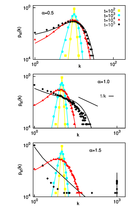
Figure 1: (Color online) Degree distribution $p(k,t)$ at four different stages of evolution: $t=10^{2}$ [(yellow) squares], $10^{3}$ [(blue) circles], $10^{4}$ [(red) triangles)] and $10^{5}$ MCS [(black) diamonds]. From top to bottom panels, subcritical ($\alpha=0.5$), critical ($\alpha=1$) and supercritical ($\alpha=1.5$) rewiring exponents. Symbols from MC simulations and corresponding solid lines from numerical integration of Eq. (1). $\beta=1$, $\langle k\rangle=10$ and $N=1000$ in all cases.

In finite networks, no node can have a degree larger than $N-1$ or lower than $0$. In fact, one would usually wish to impose a minimum nonzero degree, e.g. $k\geq 1$. The temporal evolution of the degree distribution is illustrated in Fig. 1. This shows the result of integrating Eq. (1) for $k\geq 1,$ different times, $\beta=1,$ and three different values of $\alpha$, along with the respective values obtained from Monte Carlo simulations.

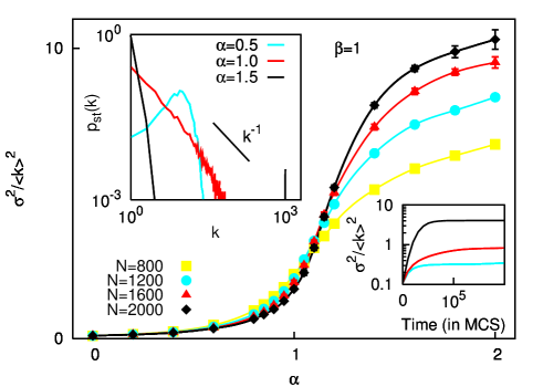
Figure 2: (Color online) Adjusted variance $\sigma^{2}/\langle k\rangle^{2}$ of the degree distribution after $2\times 10^{5}$ MCS against $\alpha$, as obtained from MC simulations, for system sizes $N=800$ [(yellow) squares], $1200$ [(blue) circles], $1600$ [(red) triangles] and $2000$ [(black) diamonds]. Top left inset shows final degree distributions for $\alpha=0.5$ [light gray (blue)], $1$ [dark gray (red)] and $1.5$ (black), with $N=1000$. Bottom right inset shows typical time series of $\sigma^{2}/\langle k\rangle^{2}$ for the same three values of $\alpha$ and $N=1200$. In all cases, $\beta=1$ and $\langle k\rangle=10$.

The main result may be summarized as follows. For $\alpha<\beta$, the network will evolve to have a characteristic size, centred around $\langle k\rangle$. At the critical case $\alpha=\beta$, all sizes appear, according either to a pure or a composite power law, as detailed above.

If we impose, say, $k\geq 1$, then starlike structures will emerge, with a great many nodes connected to just a few hubs .

Figure 2 illustrates the second order phase transition undergone by the variance of the final (stationary) degree distribution, depending on the exponent $\alpha$, where $\beta$ is set to unity. It should be mentioned that this particular case, $\beta=1$, corresponds to edges being chosen at random for disconnection, since the probability of a random edge belonging to node $i$ is proportional to $k_{i}$.

This topological phase transition is similar to the ones that have been described in equilibrium network ensembles defined via an energy function, in the so-called synchronic approach to network analysis Farkas ; Park ; Burda ; Derenyi . However, our (nonequilibrium) model does not come within the scope of this body of work, since the rewiring rates cannot, in general, be derived from a potential. Furthermore, we are here concerned with the time evolution rather than the stationary states, making our approach diachronic.

Summing up, in spite of its simplicity, our model captures the essence of many real-world networks which evolve while leaving the total numbers of nodes and edges roughly constant. The grade of heterogeneity of the stationary distribution obtained is seen to depend crucially on the relation between the exponents modelling the probabilities a node has of obtaining or loosing a new edge. It is worth mentioning that the heterogeneity of the degree distribution of a random network has been found to determine many relevant behaviours and magnitudes such as its clustering coefficient and mean minimum path Newman_rev , critical values related to the dynamics of excitable networks Johnson , or the synchronisability for systems of coupled oscillators (since this depends on the spectral gap of the Laplacian matrix) Barahona .

The above shows how scale-free distributions, with a range of exponents, may emerge for nonlinear rewiring, although only in the critical situation in which the probabilities of gaining or loosing edges are the same. We believe that this non-trivial relation between the microscopic rewiring actions (governed in our case by parameters $\alpha$ and $\beta$) and the emergent macroscopic degree distributions could shed light on a class of biological, social and communications networks.

This work was supported by Junta de Anadalucía project FQM-01505 and by Spanish MEC-FEDER project FIS2009-08451

References

- (1) S. Boccaletti et al., Phys. Rep. 424, 175 (2006)
- (2) A. Arenas et al., Phys. Rep. 469, 93 (2008)
- (3) J. Marro, J.J. Torres and J.M. Cortes, J. Stat. Mech.: Theory and Experiment, P02017 (2008)
- (4) A.-L. Barabási and R. Albert, Science 286 509–512 (1999)
- (5) G. Kossinets and D.J. Watts, Science 311, 88–90 (2006)
- (6) A.Y. Klintsova and W.T. Greenough, Current Opinion in Neurobiology 9, 203–208 (1999)
- (7) K.S. Lee, F. Schottler, M. Oliver, and G. Lynch, J. Neurophysiol. 44, 247–258 (1980)
- (8) M. De Roo, P. Klauser, P. Mendez, L. Poglia, and D. Muller, Cerebral Cortex 18 151–161 (2008)
- (9) R. Albert and A.-L. Barabási, Phys. Rev. Lett. 85, 5234 (2000)
- (10) S. Thurner, F. Kyriakopoulos, and C. Tsallis, Phys. Rev. E. 76, 036111 (2007)
- (11) P.L. Krapivsky, S. Redner, and F. Leyvraz, Phys. Rev. Lett. 85, 4629 (2000)
- (12) Although all moments of will diverge unless .
- (13) G. Bianconi and A.-L. Barabási, Phys. Rev. Lett. 86, 5632 (2001)
- (14) I. Farkas, I. Derényi, G. Palla, and T. Vicsek, Lect. Notes in Phys. 650, 163 (2004)
- (15) J. Park and M.E.J. Newman, Phys. Rev. E. 70, 066117 (2004)
- (16) Z. Burda, J. Jurkiewicz, and A. Krzywicki, Physica A 344, 56 (2004)
- (17) I. Derényi, I. Farkas, G. Palla, T. Vicsek, Physica A 344, 583 (2004)
- (18) M.E.J. Newman, SIAM Reviews 45, 167 (2003)
- (19) S. Johnson, J. Marro, and J.J. Torres, Europhys. Lett. 83, 46006 (2008)
- (20) M. Barahona and L.M. Pecora, Phys. Rev. Lett. 89, 054101 (2002)