Path integral evaluation of equilibrium isotope effects

Abstract

A general and rigorous methodology to compute the quantum equilibrium isotope effect is described. Unlike standard approaches, ours does not assume separability of rotational and vibrational motions and does not make the harmonic approximation for vibrations or rigid rotor approximation for the rotations. In particular, zero point energy and anharmonicity effects are described correctly quantum mechanically. The approach is based on the thermodynamic integration with respect to the mass of isotopes and on the Feynman path integral representation of the partition function. An efficient estimator for the derivative of free energy is used whose statistical error is independent of the number of imaginary time slices in the path integral, speeding up calculations by a factor of $\sim 60$ at $500$ $\mathrm{K}$ and more at room temperature. We describe the implementation of the methodology in the molecular dynamics package Amber 10. The method is tested on three [1,5] sigmatropic hydrogen shift reactions. Because of the computational expense, we use ab initio potentials to evaluate the equilibrium isotope effects within the harmonic approximation, and then the path integral method together with semiempirical potentials to evaluate the anharmonicity corrections. Our calculations show that the anharmonicity effects amount up to $30\%$ of the symmetry reduced reaction free energy. The numerical results are compared with recent experiments of Doering and coworkers, confirming the accuracy of the most recent measurement on 2,4,6,7,9-pentamethyl-5-(5,5-²H₂)methylene-11,11a-dihydro-12H-naphthacene as well as concerns about compromised accuracy, due to side reactions, of another measurement on 2-methyl-10-(10,10-²H₂)methylenebicyclo[4.4.0]dec-1-ene.

I Introduction

The equilibrium (thermodynamic) isotope effect (EIE) is defined as the effect of isotopic substitution on the equilibrium constant. Denoting an isotopolog with a lighter (heavier) isotope by a subscript l (h), the EIE is defined as the ratio of equilibrium constants

$$\mathrm{EIE}=\frac{K_{l}}{K_{h}}=\frac{Q_{l}^{\left(p\right)}/Q_{l}^{\left(r\right)}}{Q_{h}^{\left(p\right)}/Q_{h}^{\left(r\right)}},$$ (1)

where $Q^{\left(r\right)}$ and $Q^{\left(p\right)}$ are molecular partition functions per unit volume of reactant and product. We study a specific case of EIE - the equilibrium ratio of two isotopomers. In this case, the EIE is equal to the equilibrium constant of the isotopomerization reaction,

$$\mathrm{EIE}=K_{\mathrm{eq}}=\frac{Q^{\left(p\right)}}{Q^{\left(r\right)}},$$ (2)

where superscripts r and p refer to reactant and product isotopomers, respectively.

Usually, equilibrium isotope effects are computed only approximately:Alston et al. (1996); Anbar et al. (2005); Gawlita et al. (1994); Hill and Schauble (2008); Hrovat et al. (1997); Janak and Parkin (2003); Kolmodin et al. (2002); Munoz-Caro et al. (2003); Ruszczycky and Anderson (2009); Saunders et al. (2007); Slaughter et al. (2000); Smirnov et al. (2009); Zeller and Strassner (2002) In particular, effects due to indistinguishability of particles and rotational and vibrational contributions to the EIE are treated separately. Furthermore, the vibrational motion is approximated by a simple harmonic oscillator and the rotational motion is approximated by a rigid rotor. In general, none of the contributions, not even the indistinguishability effects can be separated from the others.Pollock and Ceperley (1987); Boninsegni and Ceperley (1995) However, at room temperature or above the nuclei can be accurately treated as distinguishable, and the indistinguishability effects can be almost exactly described by symmetry factors. On the other hand, the effective coupling between rotations and vibrations, anharmonicity of vibrations, and non-rigidity of rotations can in fact become more important at higher temperatures. For simplicity, from now on we denote these three effects together as “anharmonicity effects” and the approximation that neglects them the “harmonic approximation” (HA). In some cases the effects of anharmonicity of the Born-Oppenheimer potential surface on the value of EIE can be substantial.Torres et al. (2000) Ishimoto et al. have shown that the isotope effect on certain barrier heights can even have opposite signs, when calculated taking anharmonicity effects into account and in the HA.Ishimoto et al. (2008)

Our goal is to describe rigorously equilibria at room temperature or above. Therefore, two approximations that we make are the Born-Oppenheimer approximation and the distinguishable particle approximation (we treat indistinguishability by appropriate symmetry factors). The error due to the Born-Oppenheimer approximation was studied for H/D EIE by Bardo and Wolfsberg,Bardo and Wolfsberg (1976) and by Kleinman and Wolfsberg,Kleinman and Wolfsberg (1973) and was shown to be of the order of 1 % in most studied cases. Since we assume that nuclei are point charges, the Born-Oppenheimer approximation implies that the potential energy surface is the same for the two isotopomers. The differences of Born-Oppenheimer surfaces due to differences of nuclear volume and quadrupole of isotopes can be important for heavy elementsBigeleisen (1996); Knyazev et al. (1999); Cowan (1981), but these are not studied in this work.

Symmetry factors themselves result in an EIE equal to a rational ratio, which can be computed analytically. In order to separate the symmetry contributions from the mass contributions to the EIE, it is useful to introduce the reduced reaction free energy,

$$\Delta F^{\mathrm{red}}=-k_{B}T\ln K_{\mathrm{eq}}^{\mathrm{red}}=-k_{B}T\ln\left(\frac{s^{(r)}Q^{(p)}}{s^{(p)}Q^{(r)}}\right),$$ (3)

where $s^{(r)}$ and $s^{(p)}$ are the symmetry factors discussed in more detail in Sec. III. To include the effects of quantization of nuclear degrees of freedom beyond the HA rigorously we use the Feynman path integral representation (PI) of the partition function. The quantum reduced reaction free energy can then be computed by thermodynamic integration with respect to the mass of the isotopes. To compute the derivative of the free energy efficiently, we use a generalized virial estimator. The advantage of this estimator is that its statistical error does not increase with the number of imaginary time slices in the discretized path integral. As a consequence, converged results can be obtained in a significantly shorter simulation than with other estimators.

The ultimate goal would be to combine the path integral methodology with ab initio potentials. However, since millions of samples are required, the computational expense results in the following “compromise:” First, the equilibrium isotope effects are computed using ab initio potentials, but as usual, within the HA. Then all anharmonicity corrections are computed using the PI methodology, but with semiempirical potentials. In other words, we take advantage of the higher accuracy of the ab initio potentials to compute the harmonic contribution to the EIE and then make an assumption that the anharmonicity effects are similar for ab initio and semiempirical potentials.

After describing theoretical features of the method, we apply it to hydrocarbons used in experimental measurements of isotope effects on [1,5] sigmatropic hydrogen transfer reactions. Two of them were recently used by Doering et al. Doering and Zhao (2006); Doering and Keliher (2007) who reported equilibrium ratios of their isotopomers. This allows us to validate our calculations as well as to discuss the apparent discrepancy in measurements of Doering et al. from a theoretical point of view.

The outline of the paper is as follows: In Sec. II, we describe a rigorous quantum-mechanical methodology to compute the EIE. Section III presents the [1,5] sigmatropic hydrogen shift reactions on which we test the methodology, explains how ab initio methods can be combined with the PI to compute the EIE, and discusses in detail symmetry effects in these reactions. Section IV explains the implementation of the method in Amber 10 and describes details of calculations and error analysis of our PIMD simulations. Results of calculations are presented and compared with experiments in Sec. V. Section VI concludes the paper.

II The methodology

Thermodynamic integration

EIE can be calculated by a procedure of thermodynamic integrationChandler (1987) with respect to the mass. This method takes advantage of the relationship

$$\mathrm{EIE}=\frac{Q^{(p)}}{Q^{(r)}}=\exp\left[-\beta\int_{0}^{1}d\lambda\frac{dF\left(\lambda\right)}{d\lambda}\right],$$ (4)

where $F=-\log Q/\beta$ is the (quantum) free energy and $\lambda$ is a parameter which provides a smooth transition between isotopomers $r$ and $p$. This can be accomplished, e.g., by linear interpolation of masses of all atoms in a molecule according to the equation

$$m_{i}\left(\lambda\right)=\left(1-\lambda\right)m_{i}^{(r)}+\lambda m_{i}^{(p)}.$$ (5)

In contrast to the partition function itself, the integrand of Eq. (4)

$$\frac{dF\left(\lambda\right)}{d\lambda}=-\frac{1}{\beta}\frac{d\log Q(\lambda)}{d\lambda}=-\frac{1}{\beta}\frac{dQ(\lambda)/d\lambda}{Q(\lambda)}$$ (6)

is a thermodynamic average and therefore can be computed by either Monte Carlo or molecular dynamics simulations.

Path integral approach

Classically, the EIE is trivial and Eq. (4) can be evaluated analytically. When quantum effects are important, this simplification is not possible. To describe quantum thermodynamic effects rigorously, one can use the path integral formulation of quantum mechanics.Feynman and Hibbs (1965) In the path integral formalism, thermodynamic properties are calculated exploiting the correspondence between matrix elements of the Boltzmann operator and the quantum propagator in imaginary time.Feynman and Hibbs (1965); Pollock and Ceperley (1987) In the last decades, path integrals proved to be very useful in many areas of quantum chemistry, most recently in calculations of heat capacities,Predescu et al. (2003) rate constants,Yamamoto and Miller (2005) kinetic isotope effects,Vaníček and Miller (2007) or diffusion coefficients.Wang and Zhao (2009)

Let $N$  be the number of atoms, $D$ the number of spatial dimensions, and $P$ the number of imaginary time slices in the discretized PI ($P=1$ gives classical mechanics, $P\rightarrow\infty$ gives quantum mechanics). Then the PI representation of the partition function $Q$ in the Born-Oppenheimer approximation is

$$Q \simeq V^{-1}C\int d\mathbf{r}^{\left(0\right)}\cdots\int d\mathbf{r}^{\left(P-1\right)}\exp\left[-\beta\Phi\left(\left\{\mathbf{r}^{\left(s\right)}\right\}\right)\right],$$ (7)

$$C \equiv\left(\frac{P}{2\pi\hbar^{2}\beta}\right)^{NPD/2}\prod_{i=1}^{N}m_{i}^{PD/2}.$$ (8)

where $\mathbf{r}^{\left(s\right)}\equiv\left(\mathbf{r}_{1}^{\left(s\right)},\mathbf{r}_{2}^{\left(s\right)},\ldots,\mathbf{r}_{N}^{\left(s\right)}\right)$ is the set of Cartesian coordinates associated with the $s$${}^{\text{th}}$ time slice, and $\Phi\left(\left\{\mathbf{r}^{\left(s\right)}\right\}\right)$ is the effective potential

$$\begin{split}\Phi\left(\left\{\mathbf{r}^{\left(s\right)}\right\}\right)=\frac{P}{2\hbar^{2}\beta^{2}}\sum_{i=1}^{N}m_{i}\sum_{s=0}^{P-1}\left(\mathbf{r}_{i}^{\left(s\right)}-\mathbf{r}_{i}^{\left(s+1\right)}\right)^{2}\\ +\frac{1}{P}\sum_{s=0}^{P-1}V\left(\mathbf{r}^{\left(s\right)}\right).\end{split}$$ (9)

The $P$ particles representing each nucleus in $P$ different imaginary time slices are called “beads.” Each bead interacts via harmonic potential with the two beads representing the same nucleus in adjacent time slices and via potential $V\left(\mathbf{r}^{\left(s\right)}\right)$ attenuated by factor $1/P$ with beads representing other nuclei in the same imaginary time slice. By straightforward differentiation of Eq. (7) we obtain the so-called thermodynamic estimator (TE),Vaníček et al. (2005)

$$\begin{split}\frac{dF\left(\lambda\right)}{d\lambda}\simeq-\frac{1}{\beta}\sum_{i=1}^{N}\frac{dm_{i}}{d\lambda}\Bigg{\langle}\frac{DP}{2m_{i}}\\ -\frac{P}{2\hbar^{2}\beta}\sum_{s=0}^{P-1}\left(\mathbf{r}_{i}^{\left(s\right)}-\mathbf{r}_{i}^{\left(s+1\right)}\right)^{2}\Bigg{\rangle}.\end{split}$$ (10)

A problem with expression (10) is that its statistical error grows with the number of time slices. A similar behavior is a well known property of the thermodynamic estimator for energy,Herman et al. (1982) where the problem is caused by the kinetic part of energy.

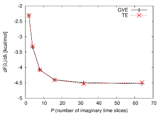
Figure 1: Convergence of the generalized virial estimator (GVE) and the thermodynamic estimator (TE) as a function of the number $P$ of imaginary time slices in the path integral. All results obtained by 1 $\mathrm{ns}$ long simulations (with the time step 0.05 $\mathrm{fs}$) of compound 1-5,5,5-d${}_{\text{3}}$ ($\lambda=0$) using GAFF force field, normal mode PIMD, and Nosé-Hoover chains of thermostats.

Generalized virial estimator

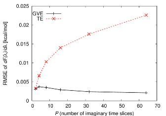
Figure 2: Root mean square errors (RMSEs) of the generalized virial estimator (GVE) and the thermodynamic estimator (TE) as a function of the number $P$ of imaginary time slices in the path integral. All results obtained by 1 $\mathrm{ns}$ long simulations (with the time step 0.05 $\mathrm{fs}$) of compound 1-5,5,5-d${}_{\text{3}}$ ($\lambda=0$) using GAFF force field, normal mode PIMD, and Nosé-Hoover chains of thermostats. Note that the RMSE of the GVE is not only non-increasing (as expected from theory), but in fact decreases slightly with increasing $P$, which is due to the decrease of correlation length.

The growth of statistical error of the thermodynamic estimator for energy is removed by expressing the estimator only in terms of the potential and its derivatives using the virial theorem.Herman et al. (1982) In our case, a similar improvement can be accomplished, if a coordinate transformation,

$$\mathbf{x}_{i}^{\left(s\right)}=m_{i}^{1/2}(\mathbf{r}_{i}^{\left(s\right)}-\mathbf{r}_{i}^{(C)}),$$ (11)

is introduced into Eq. (7) prior to performing the derivative. Here, the “centroid” coordinate is defined as

$$\mathbf{r}_{i}^{(C)}=\frac{1}{P}\sum_{s=0}^{P-1}\mathbf{r}_{i}^{(s)}.$$ (12)

In other words, first the “centroid” coordinate $\mathbf{r}_{i}^{\left(C\right)}$ is subtracted, and then the coordinates are mass-scaled. Resulting generalized virial estimator (GVE)Vaníček and Miller (2007); Vaníček and Miller (2005) takes the form

$$\begin{split}\frac{dF\left(\lambda\right)}{d\lambda}\simeq-\frac{1}{\beta}\sum_{i=1}^{N}\frac{dm_{i}/d\lambda}{m_{i}}\Bigg{[}\frac{D}{2}\\ +\frac{\beta}{2P}\left\langle\sum_{s=0}^{P-1}\left(\mathbf{r}_{i}^{(s)}-\mathbf{r}_{i}^{(C)}\right)\cdot\frac{\partial V\left(\mathbf{r}^{(s)}\right)}{\partial\mathbf{r}_{i}^{(s)}}\right\rangle\Bigg{]}.\end{split}$$ (13)

Its primary advantage is that the root mean square error (RMSE) of the average, $\sigma_{\mathrm{\text{av}}}$, is approximately independent on the number of imaginary time slices $P$,

$$\sigma_{\mathrm{\text{av}}}\approx O\left(P^{0}\tau_{\mathrm{c}}^{1/2}\tau_{\mathrm{sim}}^{-1/2}\right).$$ (14)

In this equation $\tau_{\mathrm{sim}}$ denotes the length of the simulation and $\tau_{\mathrm{c}}$ is the correlation length.

The convergence of values and statistical errors of both estimators as a function of number $P$ of imaginary time slices for systems studied in this paper is discussed in Section IV. As expected, up to the statistical error they give the same values as can be seen in Fig. 1. Nevertheless, when quantum effects are important, and a high value of $P$ must be used, the GVE is the preferred estimator since it has much smaller statistical error and therefore converges much faster than the TE (see Fig. 2).

Path integral molecular dynamics

Thermodynamic average in Eq. (13) can be evaluated efficiently using the path integral Monte Carlo (PIMC) or path integral molecular dynamics (PIMD). In PIMC, gradients of $V$ in Eq. (13) result in additional calculations since the usual Metropolis Monte Carlo procedure for the random walk only requires the values of $V$. This additional cost can be, however, reduced either by less frequent sampling, or by using a trick in which the total derivative with respect to $\lambda$ (not the gradients!) is computed by finite difference.Vaníček and Miller (2007); Vaníček and Miller (2005); Predescu et al. (2003); Predescu (2004) In case of PIMD, the presence of gradients of $V$ in Eq. (13) does not slow down the calculation since forces are already computed by a propagation algorithm. Although in principle, a PIMC algorithm for a specific problem can always be at least as efficient as a PIMD algorithm, in practice it is much easier to write a general PIMD algorithm and so PIMD is usually the algorithm used in general software packages. Since PIMD was implemented in Amber 9,Case et al. (2006) we have implemented the methodology described above for computing EIEs into Amber 10.Case et al. (2008) This implementation is what was used in calculations in the following sections. In PIMD, equation (7) is augmented by fictitious classical momenta $\boldsymbol{\mathrm{p}}^{\left(s\right)}$,

$$Q\simeq V^{-1}\tilde{C}\int d\mathbf{p}^{\left(0\right)}\cdots\int d\mathbf{p}^{\left(P-1\right)}\int d\mathbf{r}^{\left(0\right)}\cdots\int d\mathbf{r}^{\left(P-1\right)}\exp\left[-\beta\left({\displaystyle\sum_{s=0}^{P-1}}\frac{\left(\mathbf{p}^{\left(s\right)}\right)^{2}}{2m_{s}}+\Phi\left(\left\{\mathbf{r}^{\left(s\right)}\right\}\right)\right)\right].$$ (15)

The normalization prefactor $\tilde{C}$ is chosen in such a way that the original prefactor $C$ in Eq. (7) is reproduced when the momentum integrals in Eq. (15) are evaluated analytically. The partition function (15) is formally equivalent to the partition function of a classical system of cyclic polyatomic molecules with harmonic bonds. Each such molecule represents an individual atom in the original molecule and interacts with molecules representing other atoms via a potential derived from the potential of the original molecule.Chandler and Wolynes (1981) This system can be studied directly using well developed methods of the classical molecular dynamics.

Low- and high-temperature limits

It is useful to see how the general path integral expressions (4), (7), and (13) behave in the low and high temperature limits. As temperature decreases, the difference of the reduced free energies of isotopomers approaches the difference of their zero point energies (ZPEs). Therefore, still assuming that indistinguishability is correctly described by symmetry factors, the low temperature limit of the EIE is equal to

$$\mathrm{EIE_{low\mathit{T}}}=\frac{s^{\left(r\right)}}{s^{\left(p\right)}}\exp\left[-\beta\left(\varepsilon^{\left(r\right)}-\varepsilon^{\left(p\right)}\right)\right],$$ (16)

where $\varepsilon$ denotes the ZPE.

At high temperature, the system approaches its classical limit. In this limit, we can set the number of imaginary time slices $P=1$, and the EIE can be computed analytically using partition function (7), which becomes

$$\begin{split}Q_{\mathrm{class}}\simeq{\displaystyle V^{-1}\left(\frac{1}{2\pi\hbar^{2}\beta}\right)^{ND/2}\prod_{i=1}^{N}m_{i}^{D/2}}\\ \times\int d^{N}\mathbf{r}\exp\left[-\beta V\left(\mathbf{r}_{1},\ldots,\mathbf{r}_{N}\right)\right].\end{split}$$ (17)

Again, for isotopomers the mass dependent factors cancel out upon substitution into Eq. (2), along with all other terms except for the integrals. Although the Born-Oppenheimer potential surface is the same for all isotopomers, the integrals do not cancel out since the integration is not performed over the whole configuration space, but only over parts attributed to reactants or products. Particles are treated as distinguishable in the classical limit and the volumes of the configuration space corresponding to reactants and products are generally different. After the reduction, EIE becomes exactly equal to the ratio of the symmetry factors,

$$\mathrm{EIE_{\mathrm{high}\mathit{T}}}=\frac{s^{\left(r\right)}}{s^{\left(p\right)}}.$$ (18)

III Equilibrium isotope effects in three [1,5] sigmatropic hydrogen shift reactions

We examine the EIE for four related compounds. The parent compound (3Z)-penta-1,3-diene (compound 1) is the simplest molecule to model the [1,5] sigmatropic hydrogen shift reaction. Two of its isotopologs, tri-deuterated (3Z)-(5,5,5-${}^{\text{2}}$H${}_{\text{3}}$)penta-1,3-diene (1-5,5,5-d${}_{\text{3}}$) and di-deuterated (3Z)-(1,1-${}^{\text{2}}$H₂)penta-1,3-diene (1-1,1-d${}_{\text{2}}$) (see Fig. 3) were used by Roth and König to measure an unusually high value of the kinetic isotope effect (KIE) on the [1,5] hydrogen shift reaction with respect to the substitution of hydrogen by deuterium.Roth and König (1966) This result pointed to a significant role of tunneling in [1,5] sigmatropic hydrogen transfer reactions. Subsequently, much theoretical research was devoted to the study of this reaction. Here we calculate final equilibrium ratios of products of this reaction, which, to our knowledge, were not theoretically predicted so far.

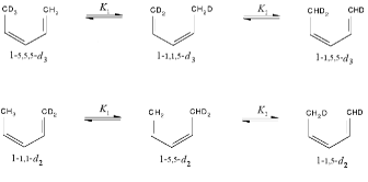
Figure 3: Equilibrium of the [1,5] hydrogen shift reaction in (3Z)-(5,5,5-${}^{\text{2}}$H${}_{\text{3}}$)penta-1,3-diene (1-5,5,5-d${}_{\text{3}}$) and in (3Z)-(1,1-${}^{\text{2}}$H₂)penta-1,3-diene (1-1,1-d${}_{\text{2}}$). If all contributions except for those due to symmetry factors $s_{a}$ and $s_{b}$ were neglected, one would obtain approximate equilibrium constants $K_{1}=3$ and $K_{2}=2$ in both cases.

Two other compounds, 2-methyl-10-(10,10-${}^{\text{2}}$H₂)methylenebicyclo[4.4.0]dec-1-ene (2-1,1-d${}_{\text{2}}$) and 2,4,6,7,9-pentamethyl-5-(5,5-${}^{\text{2}}$H₂)methylene-11,11a-dihydro-12H-naphthacene (3-1,1-d${}_{\text{2}}$) (see Fig. 4), were recently used by Doering et al. to confirm and possibly refine the experimental value of the KIE on the [1,5] hydrogen shift.Doering and Zhao (2006); Doering and Keliher (2007) In contrast to (3Z)-penta-1,3-diene (compound 1), where the s-trans conformer incompetent of the [1,5] hydrogen shift is the most stable, pentadiene moiety in compounds 2 and 3 is locked in the s-cis conformation. This not only increases the reaction rate, but also rules out the (very small) effect of the EIE on the KIE due to the shift in s-cis/s-trans equilibrium. For both molecules Doering et al. reported final equilibrium ratios of isotopomers. Despite the similarity of compounds 2 and 3, these ratios are qualitatively different. Indeed, one motivation for measuring EIE in compound 3 was that Doering et al. suspected that in the case of 2-1,1-d${}_{\text{2}}$ the equilibrium ratio might be modified by unwanted side reactions, mainly dimerizations. One of our goals is to elucidate this discrepancy from the theoretical point of view.

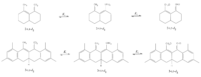
Figure 4: Equilibrium of the [1,5] hydrogen shift reaction in 2-methyl-10-(10,10-${}^{\text{2}}$H₂)methylenebicyclo[4.4.0]dec-1-ene (2-1,1-d${}_{\text{2}}$) and in 2,4,6,7,9-pentamethyl-5-(5,5-${}^{\text{2}}$H₂)methylene-11,11a-dihydro-12H-naphthacene (3-1,1-d${}_{\text{2}}$) (the locators of positions of deuterium atoms in abbreviations are chosen to correspond to locators in (3Z)-penta-1,3-diene). As for compound 1, values of equilibrium constants imposed by symmetry are $K_{1}=3$ and $K_{2}=2$.

As can be seen in Figs. 3 and 4, the final equilibrium of the [1,5] hydrogen shift reaction of all examined compounds can be described as an outcome of two reactions. The second reaction (leading from deuterio-methyl-dideuterio-methylene to dideuterio-methyl-deuterio-methylene in tri-deuterated compounds and from dideuterio-methyl-methylene to deuterio-methyl-deuterio-methylene in di-deuterated compounds) produces a mixture of species that differ by the orientation of the mono-deuterated methylene group. Due to a high barrier for rotation of this group, the two products cannot be properly sampled in a single PIMD simulation. Therefore an additional PIMD simulation is necessary, as shown on the example of 1-5,5,5-d${}_{\text{3}}$ in Fig. 5. The reduced free energy of the second step is then calculated as

$$\Delta F^{\mathrm{red}}=-k_{B}T\ln\left[\frac{K_{2}^{\mathrm{PIMD}}}{2}\left(1+K_{3}^{\mathrm{PIMD}}\right)\right],$$ (19)

where 1/2 is the ratio of symmetry factors and $K_{2}^{\mathrm{PIMD}}$ and $K_{3}^{\mathrm{PIMD}}$ stand for equilibrium constants obtained by the second and third PIMD simulations, respectively. Together they represent the second reaction step.

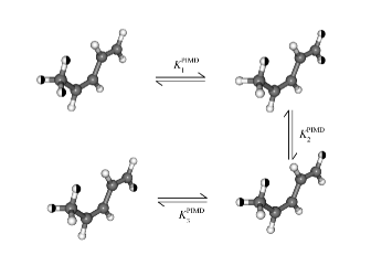
Figure 5: Three PIMD simulations used to compute equilibrium ratios of the [1,5] hydrogen shift reaction in (3Z)-(5,5,5-${}^{\text{2}}$H${}_{\text{3}}$)penta-1,3-diene (1-5,5,5-d${}_{\text{3}}$). Half white, half black spheres represent deuterium atoms. The methyl group, in contrast to methylene, rotates during simulations.

Combination of ab initio methods with the PIMD

Unfortunately, at present the PIMD method cannot be used in conjunction with higher level ab initio methods, due to a high number of potential energy evaluations needed. Semiempirical methods, which can be used instead, do not achieve comparable accuracy. We therefore make the following two assumptions: First, we assume that the main contribution to the EIE can be calculated in the framework of HA. Second, we assume that selected semiempirical methods are accurate enough to reliably estimate the anharmonicity correction. The anharmonicity correction is calculated as

$$\Delta\Delta F^{\mathrm{anharm}}=\Delta F_{\mathrm{PIMD}}^{\mathrm{red}}-\Delta F_{\mathrm{HA}}^{\mathrm{red}}.$$ (20)

With these two assumptions, we can take advantage of both PIMD and higher level methods by adding the semiempirical anharmonicity correction to the HA result calculated by a more accurate method. The HA value of $\Delta F^{\mathrm{red}}$ is obtained by Boltzmann averaging over all possible distinguishable conformations,

$${\displaystyle\Delta F_{\mathrm{HA}}^{\mathrm{red}}=-k_{B}T\ln\left[\frac{s^{(r)}\sum_{i=1}^{N_{p}}\left\{\exp\left(\frac{-E_{i}^{\mathrm{el}}}{k_{B}T}\right)\sum_{j=1}^{s^{(p)}}Q_{ij}^{\mathrm{\mathit{p,\mathrm{nuc}}}}\right\}}{s^{(p)}\sum_{i=1}^{N_{r}}\left\{\exp\left(\frac{-E_{i}^{\mathrm{el}}}{k_{B}T}\right)\sum_{j=1}^{s^{(r)}}Q_{ij}^{\mathrm{\mathit{r,\mathrm{nuc}}}}\right\}}\right]},$$ (21)

where $N_{r}$ is the number of “geometrically different isomers” of a reactant. By geometrically different isomers we mean species differing in their geometry, not species differing only in positions of isotopically substituted atoms. $E_{i}^{\mathrm{el}}$ is the electronic energy (including nuclear repulsion) of $i^{\mathrm{th}}$ isomer, $s^{(r)}$ is the symmetry factor and $Q_{ij}^{r,\mathrm{nuc}}$ are partition functions of the nuclear motion of $s^{(r)}$ isotopomers. $N_{p}$, $s^{(p)}$, $Q_{ij}^{p,\mathrm{nuc}}$ denote analogous quantities for the product.

Symmetry factors

Although symmetry effects can be computed analytically, for the reactions studied in this paper they are nontrivial and so we discuss them here in more detail. As mentioned above, we are interested in moderate temperatures (above $\sim 100$ $\mathrm{K}$) where quantum effects might be very important but the distinguishable particle approximation remains valid. In this case, effects of particle indistinguishability and of non-distinguishing several, in principle distinguishable minima, by an experiment can be conveniently unified by the concept of symmetry factor. In our setting, we will call “symmetry factor” the product

$$s=s^{\mathrm{exp}}\cdot\prod_{i=1}^{N}\frac{1}{\sigma_{i}}.$$ (22)

Here, $s^{\mathrm{exp}}$ refers to the number of distinguishable minima not distinguished by the experiment and $\sigma_{i}$ are the usual rotational symmetry numbers of symmetric rotors. The symmetry numbers are present only if either the whole molecule or some of its parts are treated as free or hindered classical symmetrical rotors. (In this case, the number of minima of the hindered rotor potential is not included in $s^{\mathrm{exp}}$.) The symmetry numbers are not present if rotational barriers are so high that the corresponding degrees of freedom should be considered as vibrations.

The concept can be illustrated on an example of the mono- and non-deuterated methyl group in a rotational potential with three equivalent minima 120$\,{}^{\circ}$ apart. At low temperatures, when hindered rotation of the methyl group reduces to a vibration, the symmetry factor is determined only by $s^{\mathrm{exp}}$. In the case of mono-deuterated methyl group there are three in principle distinguishable minima corresponding to three rotamers, which are, as we suppose, considered to be one species by the observer. Therefore $s^{\mathrm{exp}}=3$. In the case of non-deuterated methyl there is only one distinguishable minimum and $s^{\mathrm{exp}}=1$. At higher temperatures, when the methyl group can be treated as a hindered rotor, its contribution to the symmetry factor is determined only by rotational symmetry number $\sigma$, where $\sigma=1$ for a mono-deuterated methyl group and $\sigma=3$ for a non-deuterated methyl group. From definition (22), it is clear that the high and low temperature pictures are consistent and give the same ratios of symmetry factors.

Partition functions $Q^{(r)}$ and $Q^{(p)}$ needed in calculation of the reduced free energy in Eq. (3) are computed as sums of partition functions of $s^{\mathrm{(r),exp}}$ and $s^{\mathrm{(p),exp}}$ isotopomers.

IV Computational details

Ab initio, density functional, and semiempirical methods

In this subsection, we will discuss the accuracy of four electronic structure methods used in our calculations. Ab initio MP2 and the B98 density functional method,Becke (1997); Schmider and Becke (1998) both in combination with the 6-311+(2df,p) basis set, were used for calculations within the HA. Semiempirical AM1Dewar et al. (1985) and SCC-DFTBElstner et al. (1998) methods were used in both HA and PIMD calculations. This allowed us to compute the error introduced by the HA.

Aside from symmetry factors, the EIE is dominated by vibrational contributions. Therefore we concentrate mainly on the accuracy of HA vibrational frequencies. According to Merrick et al.,Merrick et al. (2007) who tested the performance of MP2 and B98 methods by means of comparison with experimental data for a set of 39 molecules, RMSE of ZPEs is 0.46 $\mathrm{kJ\cdot mol^{-1}}$ at MP2/6-311+(2df,p) and 0.31 $\mathrm{kJ\cdot mol^{-1}}$ at B98/6-311+(2df,p) level of theory. Appropriate ZPE scaling factors are equal to 0.9777 and 0.9886 respectively. Corresponding RMSEs of frequencies are 40 $\mathrm{cm^{-1}}$ and 31 $\mathrm{cm^{-1}}.$ Therefore, a slightly higher accuracy can be expected from the B98 functional. The accuracy of both semiempirical methods is significantly worse than the accuracy of higher level ab initio methods. According to Witek and Morokuma, the RMSE of AM1 frequencies in comparison to experimental values for 66 molecules is 95 $\mathrm{cm^{-1}}$ with frequency scaling factor equal to 0.9566.Witek and Morokuma (2004) The error of vibrational frequencies obtained using SCC-DFTB depends on parametrization. We tested two parameter sets: the original SCC-DFTB parametrizationElstner et al. (1998) and the parameter set optimized with respect to frequencies by Malolepsza et al.Malolepsza et al. (2005) (further designated SCC-DFTB-MWM). The error of vibrational frequencies calculated with the original SCC-DFTB parameters was studied by Krüger et al.Krüger et al. (2005) The mean absolute deviation from the reference values calculated at BLYP/cc-pVTZ for a set of 22 molecules was 75 $\mathrm{cm^{-1}}$. The error of the reference method itself, as compared to an experiment with a slightly smaller set of molecules was 31 $\mathrm{cm^{-1}}$. In the above mentioned study performed by Witek and Morokuma, RMSE of 82 $\mathrm{cm^{-1}}$ with scaling factor 0.9933 was obtained.Witek and Morokuma (2004) The SCC-DFTB-MWM mean absolute deviation of experimental and calculated frequencies for a set of 14 hydrocarbons is indeed better and is equal to 33 $\mathrm{cm^{-1}}$ instead of 59 $\mathrm{cm^{-1}}$ for the original parametrization. Malolepsza et al. (2005)

The suitability of AM1, SCC-DFTB, SCC-DFTB-MWM, and several other semiempirical methods for our systems was tested by comparison of EIE values in the HA and of potential energy scans with the corresponding quantities computed with MP2 and B98. Results of this comparison are presented in the appendix. The AM1 method is shown to reproduce ab initio EIEs in the HA very well, but fails to reproduce scans of potential energies of methyl and vinyl group rotations. Therefore, in addition to AM1 method we used the SCC-DFTB method, which is, among the semiempirical methods tested by us, the best in reproducing ab initio potential energy scans. On the other hand, compared to AM1, SCC-DFTB gives a worse EIE in the HA.

Statistical errors, convergence, and parameters of PIMD simulations

Statistical RMSEs of averages of PIMD simulations were calculated from the equation

$$\sigma_{\mathrm{av}}=\tau_{\mathrm{c}}^{1/2}\tau_{\mathrm{sim}}^{-1/2}\sigma,$$ (23)

where $\sigma$ is the RMSE of one sample. Correlation lengths $\tau_{\mathrm{c}}$ were estimated by the method of block averages.Flyvbjerg and Petersen (1989) At constant temperature, the correlation length decreases with increasing number of imaginary time slices. Also, for constant number of imaginary time slices, the correlation length decreases with increasing temperature. Finally, the correlation length stays approximately constant at different temperatures, if the number of imaginary time slices is chosen so that $\Delta F$ is converged to approximately the same precision. In our systems, correlation length is close to 3.5 $\mathrm{ps}$.

The EIE was studied at four different temperatures: 200, 441.05, 478.45, and 1000 $\mathrm{K}$ using the normal mode version of PIMD.Berne and Thirumalai (1986) To control temperature, the Nosé-Hoover chains with four thermostats coupled to each PI degree of freedom were used.Martyna et al. (1992).

Different numbers $P$ of imaginary time slices had to be used at different temperatures, since at lower temperatures quantum effects become more important, and the number of imaginary time slices necessary to maintain the desired accuracy increases. To examine the required value of $P$ as a function of temperature we used the GAFF force field.Wang et al. (2004) Whereas the accuracy of vibrational frequencies calculated using the GAFF force field is relatively low [RMS difference of GAFF and B98/6-311+(2df,p) frequencies of compound 1 is equal to 125 $\mathrm{cm^{-1}}$], the potential should be realistic enough for the assessment of the convergence with respect to $P$. For example, the difference of potential energies $\Delta E$ between s-cis and s-trans conformations of compound 1 is 4.3 $\mathrm{kcal\cdot mol^{-1}}$ as compared to 2.7 $\mathrm{kcal\cdot mol^{-1}}$ obtained by MP2/6-311+(2df,p) or 3.5 $\mathrm{kcal\cdot mol^{-1}}$ obtained by B98/6-311+(2df,p).

To check the convergence at 478.45 $\mathrm{K}$, we calculated values of the integral in Eq. (4) for the deuterium transfer reaction in 1-5,5,5-d${}_{\text{3}}$ with 40 and 48 imaginary time slices (using Simpson’s rule with 5 points). Their difference is equal to 0.00005 $\pm$ 0.00040 $\mathrm{kcal\cdot mol^{-1}}$. This is less than the statistical error of the calculation on the model system, which itself is smaller than the error of production calculations, since the model calculation was 10 times longer than the longest production calculation. Therefore, taking into account the accuracy of production calculations, $P=40$ can be considered the converged number of imaginary time slices. This is further supported by the observation of the convergence of the single value of the GVE (13) at $\lambda=0$. The relative difference of GVE values obtained with 40 and 48 imaginary time slices is equal to 0.22 $\pm$ 0.02 %, whereas the difference between 40 and 72 imaginary time slices equals to 0.39 $\pm$ 0.04 %. The discretization error is asymptotically proportional to $P^{-2}$. By fitting this dependence to the calculated values, we estimated the difference between the values for $P=40$ and for the limit $P\rightarrow\infty$ to be less than 0.6 %. This is only three times more than the difference between $P=40$ and $P=48$. Therefore, if the integral converges similarly as the GVE, we can use the aforementioned difference between 40 and 48 imaginary time slices as the criterion of convergence. The convergence of the GVE with the number of imaginary time slices is displayed in Fig. 1. Since 441.05 $\mathrm{K}$ is close enough to 478.45 $\mathrm{K}$ we used the same value of $P$ at this temperature. To check the convergence at 200 and 1000 $\mathrm{K}$, we observed only the convergence of the single value of the GVE. At 200 $\mathrm{K}$ the relative difference of GVE values at $\lambda=0$ obtained with $P=72$ and $P=80$ is 0.03 $\pm$ 0.07 %. Based on the comparison with the previous result, $P=72$ is considered sufficient. At 1000 $\mathrm{K}$, the relative difference of GVE values at $\lambda=0$ for $P=24$ and $P=32$ equals to 0.1 $\pm$ 0.02 %, so that 24 imaginary time slices are used further.

The time step at 441.05 and 478.45 $\mathrm{K}$ was 0.05 $\mathrm{fs}$ to satisfy the requirement of energy conservation. At 200 and 1000 $\mathrm{K}$, a shorter step of 0.025 $\mathrm{fs}$ was used due to the increased stiffness of the harmonic bonds between beads at 200 $\mathrm{K}$ and due to the increased average kinetic energy at 1000 $\mathrm{K}$. The simulation lengths differed for different molecules. For both isotopologs of compound 1 simulation length of 1 $\mathrm{ns}$ ensured that the system properly explored both the s-trans and the s-cis conformations. Convergence was checked by monitoring running averages and by comparing the ratio of the s-trans and s-cis conformers with the ratio calculated in the HA. The length of converged PIMD simulations of compound 2 was 500 $\mathrm{ps}$. Convergence was checked again using running averages and by visual analysis of trajectories to ensure that the system properly explored all local minima. For compound 3, the simulation length was 400 $\mathrm{ps}$.

The integral in Eq. (4) was calculated using the Simpson’s rule. Using the AM1 potential, the GVE was evaluated for five values of $\lambda$, namely for $\lambda=0.0,0.25,0.5,0.75,1.0$. Convergence was checked by comparison with values obtained using the trapezoidal rule. Since the dependence of the estimator on the parameter $\lambda$ is almost linear, the difference between the two results remained well under the statistical error. Using the SCC-DFTB potential, the dependence on $\lambda$ was less smooth. As a result, nine equidistant values of $\lambda$ were needed to achieve similar convergence. In one case, as many as 17 values of $\lambda$ had to be used.

	1${}^{\text{st}}$ step $\Delta F^{\mathrm{red}}$	$\Delta\Delta F^{\mathrm{anharm}}$	2${}^{\text{nd}}$ step $\Delta F^{\mathrm{red}}$	$\Delta\Delta F^{\mathrm{anharm}}$
(3Z)-(5,5,5-${}^{\text{2}}$H${}_{\text{3}}$)penta-1,3-diene (1-5,5,5-d${}_{\text{3}}$)
AM1 (PIMD)	0.0395	-0.0041$\pm$0.0009	-0.0154	0.0022$\pm$0.0007
SCC-DFTB (PIMD)	0.1245	-0.0039$\pm$0.0007	-0.0616	0.0026$\pm$0.0005
B98 (HA) + $\Delta\Delta F_{\mathrm{AM1}}^{\mathrm{anharm}}$	0.0587		-0.0248
MP2 (HA) + $\Delta\Delta F_{\mathrm{AM1}}^{\mathrm{anharm}}$	0.0770		-0.0338
(3Z)-(1,1-${}^{\text{2}}$H2)penta-1,3-diene (1-1,1-d${}_{\text{2}}$)
AM1 (PIMD)	-0.0283	0.0063$\pm$0.0009	0.0191	-0.0023$\pm$0.0007
SCC-DFTB (PIMD)	-0.1142	0.0049$\pm$0.0006	0.0610	-0.0017$\pm$0.0005
B98 (HA) + $\Delta\Delta F_{\mathrm{AM1}}^{\mathrm{anharm}}$	-0.0466		0.0282
MP2 (HA) + $\Delta\Delta F_{\mathrm{AM1}}^{\mathrm{anharm}}$	-0.0645		0.0372

Table 1: Reduced free energies $\Delta F^{\mathrm{red}}$ $\left[\mathrm{kcal\cdot mol^{-1}}\right]$ and anharmonicity corrections $\Delta\Delta F^{\mathrm{anharm}}$ $\left[\mathrm{kcal\cdot mol^{-1}}\right]$ of [1,5] hydrogen shift reactions in 1-5,5,5-d${}_{\text{3}}$ and in 1-1,1-d${}_{\text{2}}$ at 478.45 $\mathrm{K}$. For AM1 and SCC-DFTB methods, values calculated by PIMD are listed followed by the anharmonicity correction obtained as the difference of the PIMD and HA value. For B98 and MP2 methods, HA values corrected by the AM1 anharmonicity correction are listed. The first reaction step in the case of tri-deuterated compound leads from 1-5,5,5-d${}_{\text{3}}$ to 1-1,1,5-d${}_{\text{3}}$, which is also the reactant of the second reaction step leading to 1-1,5,5-d${}_{\text{3}}$. In case of di-deuterated compound the sequence is: 1-1,1-d${}_{\text{2}}$, 1-5,5-d${}_{\text{2}}$ and 1-1,5-d${}_{\text{2}}$.

Amber 10 implementation

The PIMD calculations were performed using Amber 10.Case et al. (2008) The part of Amber 10 code, which computes the derivative $dF\left(\lambda\right)/d\lambda$ with respect to the mass was implemented by one of us and can be invoked by setting ITIMASS variable in the input file. Several posible ways to compute the derivative are obtained by combining one of two implementations of PIMD in sander (either the multisander implementation or the LES implementation) with either the Nosé-Hoover chains of thermostats or the Langevin thermostat, with the normal mode or “primitive” PIMD, and with the TE or GVE. Calculating the value of $dF\left(\lambda\right)/d\lambda$ for compound 1-5,5,5-d${}_{\text{3}}$ using GAFF force field, at $\lambda=0$, $T=478.45$ $\mathrm{K}$, and for several values of $P$, we confirmed that all twelve possible combinations give the same result. For example, Fig. 1 shows the agreement of the GVE and TE. Nevertheless, the twelve methods differ by RMSEs of $dF\left(\lambda\right)/d\lambda$ (due to different statistical errors of estimators and correlation lengths) and by computational costs. As expected, the most important at higher values of $P$ is the difference of statistical errors of GVE and TE. Figure 2 compares the dependence of the RMSE of the GVE and TE on the number $P$ of imaginary time slices. For $P=64$, the converged simulation with GVE is approximately 100 times faster than with TE. Less significant differences of RMSEs are due to differences in correlation lengths. As expected, for primitive PIMD with Langevin thermostat the correlation length depends strongly on collision frequency $\gamma$ of the thermostat. The correlation length is approximately 450-500 $\mathrm{fs}$ for $\gamma=0.3$ $\mathrm{ps^{-1}}$, falling down quickly to 120-150 $\mathrm{fs}$ for $\gamma=3$ $\mathrm{ps^{-1}}$ and to 5 $\mathrm{fs}$ for $\gamma=300$ $\mathrm{ps^{-1}}$, then rising slowly again. This can be compared to correlation length of 10-20 $\mathrm{fs}$ of the primitive PIMD thermostated by Nosé-Hoover chains of 4 thermostats per degree of freedom. A smaller difference can be found between correlation lengths of the normal mode (3-8 $\mathrm{fs}$) and primitive PIMD (10-20 $\mathrm{fs}$).

Used software

All PIMD calculations were performed in Amber 10.Case et al. (2008) All MP2 and B98 calculations as well as AM1 and PM3 semiempirical calculations in the HA were done in Gaussian 03 revision E01.Frisch et al. DFTB and SCC-DFTB calculations in the HA used the DFTB+ code, version 1.0.1.Aradi et al. (2007) SCC-DFTB harmonic frequencies were computed numerically using analytical gradients provided by the DFTB+ code. The step size for numerical differentiation was set equal to 0.01 Å. This value was also used by Krüger et al.Krüger et al. (2005) in their study validating the SCC-DFTB method and their frequencies differed from purely analytical frequencies of Witek et al.Witek and Morokuma (2004) by at most 10 $\mathrm{cm^{-1}}$. To diagonalize the resulting numerical Hessian, we used the formchk utility included in the Gaussian program package.

V Results

V.1 (3Z)-penta-1,3-diene

(3Z)-penta-1,3-diene (compound 1) is the simplest of examined molecules. Its non-deuterated isotopolog has three distinguishable minima: the s-trans conformer, which is the global minimum and two s-cis conformers related by mirror symmetry. Strictly speaking, in pentadiene the s-cis species have actually gauche conformations due to sterical constraints. In their original experiments, Roth and König studied two isotopologs, 1-5,5,5-d${}_{\text{3}}$ and 1-1,1-d${}_{\text{2}}$. The EIEs of both isotopologs were computed using the PIMD methodology of Sec. II at 478.45 $\mathrm{K}$. Resulting reduced free energies are listed in Table 1. Note that the anharmonicity correction is very similar for AM1 and SCC-DFTB methods, even though the main part of $\Delta F^{\mathrm{red}}$ obtained in the HA ($\Delta F_{\mathrm{HA}}^{\mathrm{red}}$) substantially differs for the two methods. This indicates that the corrections are fairly reliable in this case and can be used to correct results of higher level methods obtained in the HA. The anharmonicity correction is as large as 20 % of the final value of the reduced free energy. Unfortunately, the difference between MP2 and B98 in the HA is still approximately four times larger than the anharmonicity correction.

	1-5,5,5-d${}_{\text{3}}$	1-1,1,5-d${}_{\text{3}}$	1-1,5,5-d${}_{\text{3}}$
AM1 (PIMD)	0.103	0.296	0.601
SCC-DFTB (PIMD)	0.108	0.285	0606
B98 (HA) + $\Delta\Delta F_{\mathrm{AM1}}^{\mathrm{anharm}}$	0.104	0.293	0.602
MP2 (HA) + $\Delta\Delta F_{\mathrm{AM1}}^{\mathrm{anharm}}$	0.105	0.291	0.604
	1-1,1-d${}_{\text{2}}$	1-5,5-d${}_{\text{2}}$	1-1,5-d${}_{\text{2}}$
AM1 (PIMD)	0.099	0.305	0.597
SCC-DFTB (PIMD)	0.093	0.315	0.591
B98 (HA) + $\Delta\Delta F_{\mathrm{AM1}}^{\mathrm{anharm}}$	0.097	0.307	0.596
MP2 (HA) + $\Delta\Delta F_{\mathrm{AM1}}^{\mathrm{anharm}}$	0.096	0.309	0.595

Table 2: Equilibrium ratios of [1,5] hydrogen shift reactions of 1-5,5,5-d${}_{\text{3}}$ and 1-1,1-d${}_{\text{2}}$ at 478.45 $\mathrm{K}$.

	1${}^{\text{st}}$ step $\Delta F^{\mathrm{red}}$	$\Delta\Delta F^{\mathrm{anharm}}$	2${}^{\text{nd}}$ step $\Delta F^{\mathrm{red}}$	$\Delta\Delta F^{\mathrm{anharm}}$
AM1 (PIMD)	-0.0337	0.0102$\pm$0.0013	0.0230	-0.0036$\pm$0.0010
B98 (HA) + $\Delta\Delta F_{\mathrm{AM1}}^{\mathrm{anharm}}$	-0.0496		0.0302
MP2 (HA) + $\Delta\Delta F_{\mathrm{AM1}}^{\mathrm{anharm}}$	-0.0674		0.0392

Table 3: Reduced free energies $\Delta F^{\mathrm{red}}$ $\left[\mathrm{kcal\cdot mol^{-1}}\right]$ and anharmonicity corrections $\Delta\Delta F^{\mathrm{anharm}}$ $\left[\mathrm{kcal\cdot mol^{-1}}\right]$ of the [1,5] hydrogen shift reaction in 2-methyl-10-(10,10-${}^{\text{2}}$H₂)methylenebicyclo[4.4.0]dec-1-ene (compound 2) at 441.05 $\mathrm{K}$. For AM1 method, values calculated by PIMD are listed followed by the anharmonicity correction obtained as the difference of PIMD and HA values. For B98 and MP2 methods, only HA values corrected by the AM1 anharmonicity correction are listed. The first reaction step leads from 2-1,1-d${}_{\text{2}}$ to 2-5,5-d${}_{\text{2}}$, which is also the reactant of the second reaction step leading to 2-1,5-d${}_{\text{2}}$.

Reduced free energies suggest a general preference valid for both tri- and di-deuterio species: Namely, deuterium, compared to hydrogen, prefers sp${}^{\text{3}}$ carbon of the methyl group to sp${}^{\text{2}}$ carbon of the vinyl group. This was also observed experimentally.Sunko et al. (1970); Barborak et al. (1971); Gajewski and Conrad (1979) As can be seen in the table, the preference is present already in the HA. At first sight this preference can be counter-intuitive: If we confine ourselves only to the most energetical C-H (or C-D) bond stretching modes and suppose that force constants do not change significantly upon substitution with deuterium, the deuterium should prefer the stiffest bonds. This is because more energy can be gained by substituting the stiffer sp² C-H bonds, assuming approximately the same change in reduced mass after substitution. (Recall that the energy of a vibrational mode is proportional to $\sqrt{k/\mu}$ where $k$ is the force constant and $\mu$ the reduced mass.) Considering the stretching modes only, this would be the case for isotopologs of compound 1. Nevertheless, taking into account also the bending and torsional vibrational modes, gains on the sp${}^{\text{3}}$ C-H bond side will dominate. (This “counter-intuitive” preference of heavier isotope in “softer” bonds is quite common. For examples see the inverse H/D equilibrium isotope effect in oxidative addition reactions of H${}_{\text{2}}$ to transition metal complexes,Hascall et al. (1999); Bender (1995); Abu-Hasanayn et al. (1993); Rabinovich and Parkin (1993) or the inverse ${}^{\text{16}}$O/${}^{\text{18}}$O isotope effect in metal mediated oxygen activation reaction.Smirnov et al. (2009)) As already stressed, final equilibrium concentrations are determined mainly by the symmetry factors and the aforementioned deuterium sp${}^{\text{3}}$ to sp${}^{\text{2}}$ preference manifests itself only in a small modification of the symmetry determined rational ratios, as seen in Table 2.

Temperature dependence of the reduced free energy

Temperature dependence of the reduced free energy for the first reaction step of hydrogen shift in 1-5,5,5-d${}_{\text{3}}$ is depicted in Fig. 6. Analogous temperature dependence for all other studied reactions is very similar to the dependence in this figure. At very low temperature, the reduced reaction free energy approaches the difference of ZPEs in accordance with Eq. (16). Absolute value of the reduced free energy is maximal at temperatures around 200 $\mathrm{K}$. At temperatures around 400-500 $\mathrm{K}$, where most measurements took place, the value of $\Delta F^{\mathrm{red}}$ is (by chance) close to the difference of ZPEs. At high temperatures, $\Delta F^{\mathrm{red}}$ goes to zero in accordance with the high temperature limit (18) discussed above, which is valid also in the HA as can be shown using the Teller-Redlich theorem.Angus et al. (1935); Redlich (1935) The temperature dependence of the anharmonicity correction was examined using the AM1 semiempirical method at temperatures 200 $\mathrm{K}$, 478.45 $\mathrm{K}$ and 1000 $\mathrm{K}$. The correction for the first reaction step of 1-5,5,5-d${}_{\text{3}}$ is equal to $-0.0042$ $\pm$ $0.0009$, $-0.0041$ $\pm$ $0.0009$ and $-0.0035$ $\pm$ $0.0008$ $\mathrm{kcal\cdot mol^{-1}}$, respectively. Therefore, taking into account statistical errors, the correction stays approximately constant over the wide temperature range. Since the value of $\Delta F^{\mathrm{red}}$ is decreasing in the region from 200 to 1000 $\mathrm{K}$, the relative importance of the correction is increasing.

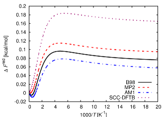
Figure 6: Reduced reaction free energies of the first step of [1,5] hydrogen shift reaction in (3Z)-(5,5,5-${}^{\text{2}}$H${}_{\text{3}}$)penta-1,3-diene (1-5,5,5-d${}_{\text{3}}$) calculated in the HA as the Boltzmann average of all s-trans and s-cis isomers.

V.2 2-methyl-10-methylenebicyclo[4.4.0]dec-1-ene

	2-1,1-d${}_{\text{2}}$	2-5,5-d${}_{\text{2}}$	2-1,5-d${}_{\text{2}}$
AM1 (PIMD)	0.098	0.306	0.595
B98 (HA) + $\Delta\Delta F_{\mathrm{AM1}}^{\mathrm{anharm}}$	0.097	0.308	0.595
MP2 (HA) + $\Delta\Delta F_{\mathrm{AM1}}^{\mathrm{anharm}}$	0.096	0.310	0.594
experimental (series 1)	0.108	0.328	0.564
experimental (series 2)	0.114	0.314	0.572

Table 4: Equilibrium ratio of the [1,5] hydrogen shift reaction in dideuterated compound 2 at 441.05 $\mathrm{K}$. Experimental series 1 and 2 were obtained by two different methods of analysis of the NMR spectrum.Doering and Zhao (2006)

	1${}^{\text{st}}$ step $\Delta F^{\mathrm{red}}$	$\Delta\Delta F^{\mathrm{anharm}}$	2${}^{\text{nd}}$ step $\Delta F^{\mathrm{red}}$	$\Delta\Delta F^{\mathrm{anharm}}$
AM1 (PIMD)	-0.0439	0.0160$\pm$0.0015	0.0265	-0.0080$\pm$0.0011
B98 (HA) + $\Delta\Delta F_{\mathrm{AM1}}^{\mathrm{anharm}}$	-0.0673		0.0376

Table 5: Reduced free energies $\Delta F^{\mathrm{red}}$ $\left[\mathrm{kcal\cdot mol^{-1}}\right]$ and anharmonicity corrections $\Delta\Delta F^{\mathrm{anharm}}$ $\left[\mathrm{kcal\cdot mol^{-1}}\right]$ of the [1,5] hydrogen shift reaction in 2,4,6,7,9-pentamethyl-5-(5,5-${}^{\text{2}}$H₂)methylene-11,11a-dihydro-12H-naphthacene (compound 3) at 441.05 $\mathrm{K}$. For AM1 method, values calculated by PIMD are listed followed by the anharmonicity correction obtained as the difference of PIMD and HA values. For B98, HA values corrected by the AM1 anharmonicity corrections are listed. The first reaction step leads from 2-1,1-d${}_{\text{2}}$ to 2-5,5-d${}_{\text{2}}$, which is also the reactant of the second reaction step leading to 2-1,5-d${}_{\text{2}}$.

Compound 2-1,1-d${}_{\text{2}}$ was used relatively recently by Doering and ZhaoDoering and Zhao (2006) to refine the original results of Roth and König. Doering and Zhao reported the equilibrium concentrations at three temperatures, from which we have chosen the lowest, $T=441.05$ $\mathrm{K}$. Since AM1 and SCC-DFTB methods gave similar anharmonicity corrections for compound 1, we used only the AM1 method in this case. Four minima were found. Energy differences between the global minimum and local minima at the B98/6-311+(2df,p) level of theory are 4.8, 7.5 and 9.5 $\mathrm{kcal\cdot mol^{-1}}$. Resulting $\Delta F^{\mathrm{red}}$ calculated according to Eq. (21) are listed in Table 3. As expected, they are similar to $\Delta F^{\mathrm{red}}$ of 1-1,1-d${}_{\text{2}}$. Anharmonicity corrections changed more and they are about 60 % higher in the absolute value.

Calculated equilibrium ratios are listed in Table 4 together with experimental ratios reported by Doering and Zhao. Theoretical and experimental ratios differ substantially, which suggests that side reactions suspected by Doering and Zhao had indeed occurred and influenced the accuracy of results of their study.

V.3 2,4,6,7,9-pentamethyl-5-methylene-11,11a-dihydro-12H-naphthacene

In order to suppress unwanted side reactions suspected for compound 2,Doering and Zhao (2006) Doering and Keliher further developed the model compound into 3-1,1-d${}_{\text{2}}$ by adding methyl substituted aromatic rings on both sides of the cyclic part.Doering and Keliher (2007) With this compound they obtained the same equilibrium ratios for all temperatures they had examined.Doering and Keliher (2007) Because of this and because the temperature 441.05 $\mathrm{K}$ we have chosen for our analysis of compound 2 differs from one of temperatures used in Ref. Doering and Keliher, 2007 by less than 2 $\mathrm{K}$, we have decided to use this temperature also for compound 3. In the HA, only the B98 density functional method was used, due to a considerable size of the molecule. Because of the increased rigidity imposed by aromatic rings on the sides of the original bi-cyclic compound, only three distinct minima were found. (We neglected several possible orientations of two methyl groups distant from the reaction site, which hardly affect the final result.) At the B98/6-311+G(2df,p) level, the local minima have energies 1.3 and 5.6 $\mathrm{kcal\cdot mol^{-1}}$ above the global minimum. The AM1 method gives the opposite order of the first and second lowest minima. Reduced free energies and anharmonicity corrections obtained using the AM1 method are listed in Table 5.

Values of both $\Delta F^{\mathrm{red}}$ and the anharmonicity corrections are again qualitatively similar (but higher in absolute values) to those of the smaller and less strained compound 2. Here, values of anharmonicity corrections reached approximately 30 % of the values of reduced free energies of both reaction steps. Resulting equilibrium ratios together with their experimental values can be seen in Table 6. Agreement of the theoretical prediction with the experimental result is very good. An uncorrected B98 HA value is also included in Table 6, to demonstrate how the anharmonicity correction modifies the HA equilibrium ratio. Surprisingly, the direct AM1 PIMD calculation is closest to the experimental value, but this ought to be ascribed to a fortunate coincidence, considering the aforementioned accuracy of electronic structure methods used in our study.

	3-1,1-d${}_{\text{2}}$	3-5,5-d${}_{\text{2}}$	3-1,5-d${}_{\text{2}}$
AM1 (PIMD)	0.098	0.308	0.595
B98 (HA)	0.095	0.312	0.593
B98 (HA) + $\Delta\Delta F_{\mathrm{AM1}}^{\mathrm{anharm}}$	0.096	0.310	0.594
experimental	0.098	0.308	0.594

Table 6: Equilibrium ratios of the [1,5] hydrogen shift reaction in compound 3 at 441.05 $\mathrm{K}$.

VI Discussion and conclusions

To conclude, the combination of higher level methods in the HA with PIMD using semiempirical methods for the rigorous treatment of effects beyond the HA proved to be a viable method for accurate calculations of EIEs. Using the generalized virial estimator for the derivative of the free energy with respect to the mass we were able to obtain accurate results at lower temperatures in reasonable time ($\sim 60$ times faster than with thermodynamic estimator), since the statistical error is independent on the number of imaginary time slices. Two semiempirical methods, AM1 and SCC-DFTB, were used for calculation of the anharmonicity correction, both giving very similar results. Calculations showed, that the anharmonicity effects account up to 30 % of the final value of the reduced free energy of considered reactions. The anharmonicity correction always decreases the absolute value of the reduced reaction free energy. This is consistent with the qualitative picture in which higher vibrational frequencies of hydrogens are lowered by the anharmonicity of a potential more than lower frequencies of deuteriums. This in turn is due to a higher amplitude of vibrations of lighter hydrogen atoms. The lower difference between frequencies of unsubstituted and deuterated species results in the lower absolute value of the reduced reaction free energy. Unfortunately, the inaccuracy of the ab initio electronic structure methods used in our study is still of at least the same order as the anharmonicity corrections.

For isotopologs of compound 1, we predicted equilibrium ratios and free energies of the [1,5] sigmatropic hydrogen shift reaction. A comparison with experimental results was not possible due to a low precision of the original measurement. For compound 2, the disagreement between theoretical and experimental data supports the suspicion by authors of the measurement that the accuracy of their results was compromised by dimerization side reactions. On the other hand, the agreement of theoretically calculated ratios with experimental observations in the case of compound 3 suggests that the isolation of the [1,5] hydrogen shift reaction from disturbing influences was successfully achieved and the observed EIE and KIE can be considered reliable.

Appendix A Examination of semiempirical methods used in PIMD simulations

To determine the suitability of semiempirical methods used in our PIMD calculations, we first compared values of the EIE in the HA. The B98 and MP2 methods served as a reference. As can be seen from Fig. 6 in the paper, which shows the temperature dependence of $\Delta F^{\mathrm{red}}$ of the first step of deuterium transfer reaction in 1-5,5,5-d${}_{\text{3}}$, the difference between B98 and MP2 at temperatures below 500 $\mathrm{K}$ is close to 0.02 kcal/mol. So is the difference between AM1 and B98 methods. On the other hand, the SCC-DFTB method clearly overestimates the extent of EIE compared to both higher level methods. A very similar trend was observed in all examined reactions. Other semiempirical methods tested were PM3Stewart (1989) and SCC-DFTB-MWM, which are not included in Fig. 6 in the paper for clarity. The PM3 method overestimates the EIE similarly to SCC-DFTB, whereas the SCC-DFTB-MWM curve is somewhat closer to ab initio curves than the SCC-DFTB one. To conclude, from this point of view AM1 is the preferred semiempirical method.

During simulations, the pentadiene molecule often passes two potential energy barriers. These are the barrier for the hindered rotation of the methyl group and the barrier for the rotation of the vinyl group, which connects s-trans and s-cis conformations. Relaxed potential energy scans of these two motions were employed as the second criterion to assess the relevancy of semiempirical methods. Methods tested were MP2, B98, AM1, SCC-DFTB, SCC-DFTB-MWM, PM3, RM1,Rocha et al. (2006) PM3CARB-1,McNamara et al. (2004) PDDG/PM3,Repasky et al. (2002) and PM6.Stewart (2007a) Potential surface scans with PM3CARB1, RM1, PM3/PDDG methods were calculated using the public domain code MOPAC 6. PM6 potential surface scans were performed in MOPAC 2007.Stewart (2007b) Results for the methyl group rotation are shown in Fig. 7. The height of the AM1 barrier is only 0.005 $\mathrm{kcal\cdot mol^{-1}}$. Moreover, positions of minima do not agree with B98 and MP2. On the other hand, the SCC-DFTB method matches higher level methods closely. From other semiempirical methods PM3 performs best in this aspect. The height of the barrier is relatively well reproduced also by PDDG/PM3, RM1 and SCC-DFTB-MWM methods, but positions of extrema of the potential energy surface are incorrect.

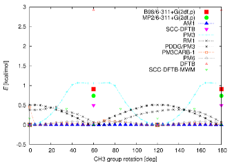
Figure 7: Relaxed potential energy scan of the methyl rotation in s-trans (3Z)-penta-1,3-diene (compound 1). For MP2, B98, DFTB, SCC-DFTB and SCC-DFTB-MWM only positions and potential energies of minima and maxima are indicated.

Figure 8 shows potential energy scans of the s-trans/s-cis rotation of the vinyl group. Again, the SCC-DFTB method matches higher level methods closely. All other methods (with the exception of DFTB) give too low barrier heights as well as too low energy differences between s-trans and s-cis conformations. Also note that the potential energy surfaces of PM3 and related methods (PDDG/PM3 and PM3CARB-1) are not smooth in the gauche region. This peculiarity of the PM3 potential surface can be seen also in the potential surface scan performed by Liu et al.Liu et al. (1993)

Figure 8: Relaxed potential energy scan of the vinyl group rotation in s-trans (3Z)-penta-1,3-diene (compound 1). For MP2, B98, DFTB, SCC-DFTB and SCC-DFTB-MWM only positions and potential energies of minima and transition states are indicated.

Based on these results we concluded that none of the semiempirical methods except for SCC-DFTB is able to sufficiently improve the AM1 potential energy surface. Whereas the frequency optimized variant of the SCC-DFTB method (SCC-DFTB-MWM) improves the EIE in the HA, it does not retain the SCC-DFTB accuracy in the potential surface scans. Hence we decided to use the AM1 and SCC-DFTB potentials for PIMD calculations. To conclude, AM1 performs very well in HA, but it cannot properly describe potential surfaces of the two rotational motions realized during simulations. On the other hand, SCC-DFTB gives worse results in HA, but it reproduces both barriers very well.

References

- Alston et al. (1996) W. C. Alston, K. Haley, R. Kanski, C. J. Murray, and J. Pranata, J. Am. Chem. Soc. 118, 6562 (1996).
- Anbar et al. (2005) A. Anbar, A. Jarzecki, and T. Spiro, Geochim. Cosmochim. Acta 69, 825 (2005).
- Gawlita et al. (1994) E. Gawlita, V. E. Anderson, and P. Paneth, Eur. Biophys. J. 23, 353 (1994).
- Hill and Schauble (2008) P. S. Hill and E. A. Schauble, Geochim. Cosmochim. Acta 72, 1939 (2008).
- Hrovat et al. (1997) D. A. Hrovat, J. H. Hammons, C. D. Stevenson, and W. T. Borden, J. Am. Chem. Soc. 119, 9523 (1997).
- Janak and Parkin (2003) K. E. Janak and G. Parkin, Organometallics 22, 4378 (2003).
- Kolmodin et al. (2002) K. Kolmodin, V. B. Luzhkov, and J. Aqvist, J. Am. Chem. Soc. 124, 10130 (2002).
- Munoz-Caro et al. (2003) C. Munoz-Caro, A. Nino, J. Z. Davalos, E. Quintanilla, and J. L. Abboud, J. Phys. Chem. A 107, 6160 (2003).
- Ruszczycky and Anderson (2009) M. W. Ruszczycky and V. E. Anderson, J. Mol. Struct. THEOCHEM 895, 107 (2009).
- Saunders et al. (2007) M. Saunders, M. Wolfsberg, F. A. L. Anet, and O. Kronja, J. Am. Chem. Soc. 129, 10276 (2007).
- Slaughter et al. (2000) L. M. Slaughter, P. T. Wolczanski, T. R. Klinckman, and T. R. Cundari, J. Am. Chem. Soc. 122, 7953 (2000).
- Smirnov et al. (2009) V. V. Smirnov, M. P. Lanci, and J. P. Roth, J. Phys. Chem. A 113, 1934 (2009).
- Zeller and Strassner (2002) A. Zeller and T. Strassner, Organometallics 21, 4950 (2002).
- Pollock and Ceperley (1987) E. L. Pollock and D. M. Ceperley, Phys. Rev. B 36, 8343 (1987).
- Boninsegni and Ceperley (1995) M. Boninsegni and D. M. Ceperley, Phys. Rev. Lett. 74, 2288 (1995).
- Torres et al. (2000) L. Torres, R. Gelabert, M. Moreno, and J. Lluch, J. Phys. Chem. A 104, 7898 (2000).
- Ishimoto et al. (2008) T. Ishimoto, Y. Ishihara, H. Teramae, M. Baba, and U. Nagashima, J. Chem. Phys. 128, 184309 (2008).
- Bardo and Wolfsberg (1976) R. D. Bardo and M. Wolfsberg, J. Phys. Chem. 80, 1068 (1976).
- Kleinman and Wolfsberg (1973) L. I. Kleinman and M. Wolfsberg, J. Chem. Phys. 59, 2043 (1973).
- Bigeleisen (1996) J. Bigeleisen, J. Am. Chem. Soc. 118, 3676 (1996).
- Knyazev et al. (1999) D. A. Knyazev, G. K. Semin, and A. V. Bochkarev, Polyhedron 18, 2579 (1999).
- Cowan (1981) R. D. Cowan, The Theory of Atomic Structure and Spectra, Los Alamos Series in Basic and Applied Sciences (University of California Press, 1981).
- Doering and Zhao (2006) W. V. Doering and X. Zhao, J. Am. Chem. Soc. 128, 9080 (2006).
- Doering and Keliher (2007) W. V. Doering and E. J. Keliher, J. Am. Chem. Soc. 129, 2488 (2007).
- Chandler (1987) D. Chandler, Introduction to modern statistical mechanics (Oxford University Press, New York, 1987).
- Feynman and Hibbs (1965) R. Feynman and A. Hibbs, Quantum Mechanics and Path Integrals, International Series in Pure and Applied Physics (McGraw-Hill, 1965).
- Predescu et al. (2003) C. Predescu, D. Sabo, J. D. Doll, and D. L. Freeman, J. Chem. Phys. 119, 10475 (2003).
- Yamamoto and Miller (2005) T. Yamamoto and W. H. Miller, J. Chem. Phys. 122, 044106 (2005).
- Vaníček and Miller (2007) J. Vaníček and W. H. Miller, J. Chem. Phys. 127, 114309 (2007).
- Wang and Zhao (2009) W. Wang and Y. Zhao, J. Chem. Phys. 130, 114708 (2009).
- Vaníček et al. (2005) J. Vaníček, W. H. Miller, J. F. Castillo, and F. J. Aoiz, J. Chem. Phys. 123, 054108 (2005).
- Herman et al. (1982) M. F. Herman, E. J. Bruskin, and B. J. Berne, J. Chem. Phys. 76, 5150 (1982).
- Vaníček and Miller (2005) J. Vaníček and W. H. Miller, in Proceedings of the Eighth International Conference: Path Integrals from Quantum Information to Cosmology, edited by C. Burdik, O. Navratil, and S. Posta (JINR Dubna, 2005).
- Predescu (2004) C. Predescu, Phys. Rev. E 70, 066705 (2004).
- Case et al. (2006) D. Case, T. Darden, I. T.E. Cheatham, C. Simmerling, R. D. J. Wang, R. Luo, K. Merz, D. Pearlman, M. Crowley, R. Walker, et al., Amber 9 (2006), University of California, San Francisco.
- Case et al. (2008) D. Case, T. Darden, I. T.E. Cheatham, C. Simmerling, J. Wang, R. Duke, R. Luo, M. Crowley, R.C.Walker, W. Zhang, et al., Amber 10 (2008), University of California, San Francisco.
- Chandler and Wolynes (1981) D. Chandler and P. G. Wolynes, J. Chem. Phys. 74, 4078 (1981).
- Roth and König (1966) W. R. Roth and J. König, J. Liebigs Ann. Chem. 699, 24 (1966).
- Becke (1997) A. D. Becke, J. Chem. Phys. 107, 8554 (1997).
- Schmider and Becke (1998) H. L. Schmider and A. D. Becke, J. Chem. Phys. 108, 9624 (1998).
- Dewar et al. (1985) M. J. S. Dewar, E. G. Zoebisch, E. F. Healy, and J. J. P. Stewart, J. Am. Chem. Soc. 107, 3902 (1985).
- Elstner et al. (1998) M. Elstner, D. Porezag, G. Jungnickel, J. Elsner, M. Haugk, T. Frauenheim, S. Suhai, and G. Seifert, Phys. Rev. B 58, 7260 (1998).
- Merrick et al. (2007) J. Merrick, D. Moran, and L. Radom, J. Phys. Chem. A 111, 11683 (2007).
- Witek and Morokuma (2004) H. A. Witek and K. Morokuma, J. Comput. Chem. 25, 1858 (2004).
- Malolepsza et al. (2005) E. Malolepsza, H. A. Witek, and K. Morokuma, Chem. Phys. Lett. 412, 237 (2005).
- Krüger et al. (2005) T. Krüger, M. Elstner, P. Schiffels, and T. Frauenheim, J. Chem. Phys. 122, 114110 (2005).
- Flyvbjerg and Petersen (1989) H. Flyvbjerg and H. G. Petersen, J. Chem. Phys. 91, 461 (1989).
- Berne and Thirumalai (1986) B. J. Berne and D. Thirumalai, Annu. Rev. Phys. Chem. 37, 401 (1986).
- Martyna et al. (1992) G. J. Martyna, M. L. Klein, and M. Tuckerman, J. Chem. Phys. 97, 2635 (1992).
- Wang et al. (2004) J. Wang, R. M. Wolf, J. W. Caldwell, P. A. Kollman, and D. A. Case, J. Comput. Chem. 25, 1157 (2004).
- (51) M. J. Frisch, G. W. Trucks, H. B. Schlegel, G. E. Scuseria, M. A. Robb, J. R. Cheeseman, J. A. Montgomery, Jr., T. Vreven, K. N. Kudin, J. C. Burant, et al., Gaussian 03, Revision E.01, Gaussian, Inc., Wallingford, CT, 2004.
- Aradi et al. (2007) B. Aradi, B. Hourahine, and T. Frauenheim, J. Phys. Chem. A 111, 5678 (2007).
- Sunko et al. (1970) D. E. Sunko, K. Humski, R. Malojcic, and S. Borcic, J. Am. Chem. Soc. 92, 6534 (1970).
- Barborak et al. (1971) J. C. Barborak, S. Chari, and P. v. R. Schleyer, J. Am. Chem. Soc. 93, 5275 (1971).
- Gajewski and Conrad (1979) J. J. Gajewski and N. D. Conrad, J. Am. Chem. Soc. 101, 6693 (1979).
- Hascall et al. (1999) T. Hascall, D. Rabinovich, V. J. Murphy, M. D. Beachy, R. A. Friesner, and G. Parkin, J. Am. Chem. Soc. 121, 11402 (1999).
- Bender (1995) B. R. Bender, J. Am. Chem. Soc. 117, 11239 (1995).
- Abu-Hasanayn et al. (1993) F. Abu-Hasanayn, K. Krogh-Jespersen, and A. S. Goldman, J. Am. Chem. Soc. 115, 8019 (1993).
- Rabinovich and Parkin (1993) D. Rabinovich and G. Parkin, J. Am. Chem. Soc. 115, 353 (1993).
- Angus et al. (1935) W. R. Angus, C. R. Bailey, J. B. Hale, C. K. Ingold, A. H. Leckie, C. G. Raisin, J. W. Thompson, and C. L. Wilson, J. Chem. Soc. 62, 971 (1935).
- Redlich (1935) O. Redlich, Z. Phys. Chem. Abt. B 28, 371 (1935).
- Stewart (1989) J. J. P. Stewart, J. Comput. Chem. 10, 209 (1989).
- Rocha et al. (2006) G. B. Rocha, R. O. Freire, A. M. Simas, and J. J. P. Stewart, J. Comput. Chem. 27, 1101 (2006).
- McNamara et al. (2004) J. P. McNamara, A.-M. Muslim, H. Abdel-Aal, H. Wang, M. Mohr, I. H. Hillier, and R. A. Bryce, Chem. Phys. Lett. 394, 429 (2004).
- Repasky et al. (2002) M. P. Repasky, J. Chandrasekhar, and W. L. Jorgensen, J. Comput. Chem. 23, 1601 (2002).
- Stewart (2007a) J. Stewart, J. Mol. Model. 13, 1173 (2007a).
- Stewart (2007b) J. J. P. Stewart, Mopac 2007 (2007b), Stewart Computational Chemistry, Colorado Springs, CO, USA.
- Liu et al. (1993) Y. P. Liu, G. C. Lynch, T. N. Truong, D. H. Lu, D. G. Truhlar, and B. C. Garret, J. Am. Chem. Soc. 115, 2408 (1993).