Efficient evaluation of accuracy of molecular quantum dynamics using dephasing representation

Abstract

Ab initio methods for electronic structure of molecules have reached a satisfactory accuracy for calculation of static properties, but remain too expensive for quantum dynamical calculations. We propose an efficient semiclassical method for evaluating the accuracy of a lower level quantum dynamics, as compared to a higher level quantum dynamics, without having to perform any quantum dynamics. The method is based on dephasing representation of quantum fidelity and its feasibility is demonstrated on the photodissociation dynamics of CO₂. We suggest how to implement the method in existing molecular dynamics codes and describe a simple test of its applicability.

Ab initio methods for electronic structure of molecules have reached a satisfactory accuracy for calculation of static properties, such as energy barriers or force constants at local minima of the potential energy surface (PES). The most accurate of such methods remain out of reach when one wants to describe molecular properties depending on the full quantum dynamics Clary (2008). To make a calculation feasible, one has to approximate the dynamics of the system Makri (1999); Miller (2005) or the PES Clary (2008), but both approaches can have nontrivial effects on the result Rabitz (1987). We consider only the second approach, in which quantum dynamics is done exactly but on a PES obtained by a lower level electronic structure method that is less accurate but also less expensive. When such a calculation is finished, its accuracy is not known because of the forbidding expense of the dynamics on the more accurate potential. In this Letter, we propose an efficient and accurate semiclassical (SC) method for evaluating the accuracy of the lower level quantum dynamics without having to perform the higher level quantum dynamics. Since our method does not even require computing the lower level quantum dynamics, it can also be used to justify, in advance, investing computational resources into the lower level calculations.

For simplicity, we use the Born-Oppenheimer approximation and focus on the quantum dynamics of nuclei, although our method applies to any quantum dynamics and should be valid even when nonadiabatic effects are important. The time-dependent Schrödinger equation is solved in two stages: First, the time-independent equation for electrons is solved with fixed nuclear configurations, and then nuclear motion is calculated on the resulting electronic PES. We consider three PESs: $V_{\text{exact}}$ is the exact PES that describes our system. $V_{\text{acc}}$ is a very accurate high-level electronic structure PES (presumably “almost exact”), which is too expensive to be used for quantum dynamics. $V_{\text{appr}}$ is an approximate PES, obtained by a lower-level electronic structure method (or by an analytical fit of $V_{\text{acc}}$) and “cheap” enough to be used for quantum dynamics.

Various quantities can describe different time-dependent features of a quantum system, but a single quantity that includes all information about the system is the time-dependent wave function, $\psi(t)$. One way to evaluate the accuracy of quantum dynamics on the approximate PES would therefore be to compute the quantum-mechanical (QM) overlap $f_{\text{QM}}(t):=\langle\psi_{\text{exact}}(t)|\psi_{\text{appr}}(t)\rangle$, where the subscript of $\psi$ denotes the corresponding PES used for propagating the initial state $\psi(0)$. The quantity $F(t):=\left|f_{\text{QM}}(t)\right|^{2}$ is known as quantum fidelity or Loschmidt echo, and has been defined by Peres Peres (1984) to measure the sensitivity of quantum dynamics to perturbations. Much effort has been devoted to the study of temporal decay of fidelity and many universal regimes have been found Gorin et al. (2006). In our setting, if $F(t)\approx 1$ for all times up to $t_{\text{max}}$, we can trust quantum dynamics on the approximate potential $V_{\text{appr}}$ and use the resulting $\psi_{\text{appr}}(t)$ to compute all dynamical properties up to $t_{\text{max}}$. In calculations, we do not know $V_{\text{exact}}$ and must use the accurate potential $V_{\text{acc}}$, and so we approximate $f_{\text{QM}}$ by

$$f_{\text{QM}}:=\left\langle\psi_{\text{acc}}(t)|\psi_{\text{appr}}(t)\right\rangle.$$ (1)

Since $V_{\text{acc}}$ is too expensive, $\psi_{\text{acc}}(t)$ cannot be computed. We describe a method which gives an accurate estimate of $f_{\text{QM}}$ without having to compute $\psi_{\text{acc}}(t)$ nor $\psi_{\text{appr}}(t)$.

The method is based on the dephasing representation (DR) of quantum fidelity, a SC approximation proposed by one of us to evaluate fidelity in chaotic, integrable, and mixed systems even in nonuniversal regimes sensitive to the initial state and details of dynamics Vaníček (2004a, 2006). Presently, we are interested in a specific type of “perturbation,” namely the difference $\Delta V=V_{\text{appr}}-V_{\text{acc}}$ between the approximate and accurate PESs. The DR of fidelity amplitude is an interference integral

$$f_{\text{DR}}(t) :=\int dx^{0}\,\rho_{\text{W}}(x^{0})\exp\left[-i\Delta S(x^{0},t)/\hbar\right],$$ (2)

$$\Delta S(x^{0},t) =\int_{0}^{t}d\tau\,\Delta V\left[q_{\text{acc}}^{\tau}(x^{0})\right].$$ (3)

Here $x$ denotes a point $\left(q,p\right)$ in phase space, the superscript is the corresponding time, $\Delta S(x^{0},t)$ is the action due to $\Delta V$ along the trajectory $q_{\text{acc}}^{t}(x^{0})$ of $V_{\text{acc}}$, and $\rho_{\text{W}}$ is the Wigner function of the initial state $\psi$,

$$\rho_{\text{W}}(x)=h^{-d}\int d\xi\mathbf{\,}\psi^{\ast}\left(q+\frac{\xi}{2}\right)\psi\left(q-\frac{\xi}{2}\right)\,\exp\left(i\frac{\xi\cdot p}{\hbar}\right).$$

In “dephasing representation,” all of fidelity decay appears to be due to interference and none due to decay of classical overlaps.

Surprising accuracy of the DR was justified by the shadowing theorem Vaníček (2004a), or, in the case of the initial state $\psi(0)$ supported by a Lagrangian manifold, by the structural stability of manifolds Cerruti and Tomsovic (2002). Interestingly, validity of the DR goes much beyond validity of the SC approximation for quantum dynamics on $V_{\text{acc}}$ or $V_{\text{appr}}$. Qualitatively, this is due to mitigating the “sign problem” of quantum or SC dynamics: large actions needed for dynamics on $V_{\text{acc}}$ or $V_{\text{appr}}$ are replaced by much smaller actions $\Delta S$ needed for fidelity calculation. Rapid oscillations in the SC expression for the dynamics on $V_{\text{acc}}$ or $V_{\text{appr}}$ are replaced by much slower oscillations in the DR. In a chaotic system where $\sim 10^{35}$ trajectories would be needed for computing $\psi_{\text{acc}}(t)$ semiclassically, as few as $1000$ trajectories were sufficient to compute fidelity amplitude Vaníček and Heller (2003). Accuracy of DR was explored numerically in Refs. Vaníček (2004a, b, 2006) which suggest that $F_{\text{DR}}$ starts to deviate from $F_{\text{QM}}$ after the Heisenberg time $t_{H}=\hbar/\Delta E$ where $\Delta E$ is the mean level spacing. Errors of DR can be estimated analytically, suggesting that DR breaks down for very large perturbations, when the effective perturbation is larger than the square root of the effective Planck’s constant Vaníček et al. (2009). However, DR remains accurate for fairly large perturbations, even when corresponding classical trajectories of $V_{\text{acc}}$ and $V_{\text{appr}}$ are completely different Vaníček (2004a, b, 2006).

The fundamental reason why quantum dynamics calculations are expensive is nonlocality of quantum mechanics: Wave function $\psi(t+\Delta t)$ at any point in space depends in general on $\psi(t)$ in the whole space. There are many computational methods for quantum dynamics, but for the sake of demonstration, we consider two methods that represent two very different general approaches.

The first approach starts with the construction of a global PES, with a computational cost $cn^{d}$ where $c$ is the cost of a single potential evaluation, $d$ is the number of degrees of freedom (DOF), and $n$ is the number of grid points in each DOF. Once the PES is known, dynamics can be performed, e.g., by the split-operator method Feit et al. (1982). In this method, the quantum evolution operator for time step $\Delta t$ is approximated by

$$e^{-iH\Delta t/\hbar}=e^{-iT\Delta t/\hbar}e^{-iV\Delta t/\hbar}+O(\Delta t^{2}),$$

where $H=T+V$ is the Hamiltonian of the system and $T$ is the kinetic energy operator. Quantum dynamics consists of alternate kinetic and potential propagations (which are just multiplications in momentum and coordinate representations, respectively) and a fast Fourier transform (FFT) to switch the representation in between. The complexity of FFT is $O(N\log N)$ where $N=n^{d}$ denotes the dimension of the Hilbert space, so the cost of propagation is $O(d\,t\,n^{d}\log n)$. Note that the same number of potential energy evaluations is required no matter how long the propagation is. This becomes an advantage for long-time dynamics calculations and a disadvantage for short-time ones. Finally, memory requirements make this approach feasible only for very small systems.

In the second approach, potential energy is calculated “on the fly” only in the vicinity of the propagated wave packet. At each time step, the cost is $c\,\tilde{n}^{d}$ where $\tilde{n}$ is the number of grid points in each DOF on which $\psi(t)$ is not negligible. Presumably, $\tilde{n}\ll n$, but the exponential scaling with $d$ remains. Assuming that $\log\tilde{n}<c$, the cost of actual propagation (e.g., by FFT) is negligible to the cost of potential evaluation, and the overall cost of the dynamics is $O(c\,\tilde{n}^{d}\,t)$.

In the DR, potential energy and forces can also be evaluated on the fly, along classical trajectories. But at each time step, the cost is only $O(d\,c\,n_{\text{paths}})$ where $n_{\text{paths}}$ is the number of classical trajectories used. The “hidden cost” in usual SC approximations is the strong dependence of $n_{\text{paths}}$ on $t$, $d$, or the type of dynamics. In Ref. [8], it was shown rigorously that $n_{\text{paths}}=C(F_{\text{DR}})\sigma^{-2}$ where $F_{\text{DR}}$ is the value of fidelity one wants to simulate, $\sigma_{F_{\text{DR}}}$ is the error (due to finite $n_{\text{paths}}$) that one wants to reach, and $0\leq C\leq 3$. Consequently, for given $F_{\text{DR}}$ and $\sigma$, the required number of trajectories is independent of $t$, $d$, or the type of dynamics! It was also shown that when $F\rightarrow 1$, which is most interesting in our application, $C\rightarrow 0$, i.e., $n_{\text{paths}}$ needed for convergence of $F_{\text{DR}}$ becomes even smaller. The overall cost of the DR dynamics is $O(d\,c\,n_{\text{paths}}\,t)$. In particular, there is no exponential scaling with the number of DOF or time.

Clearly, DR is faster than the construction of a global PES and than the quantum dynamics on the fly. Only at very long times $t$, in the first quantum approach, since the global PES is already constructed, the cost of propagation becomes dominant and one would expect that QM dynamics would beat DR dynamics which requires new potential evaluations. But even then the ratio of the costs of DR and QM is $c\,n_{\text{paths}}/n^{d}\log n$. Assuming that the number of nuclear DOF is comparable to the number of electronic DOF, then even for the most accurate ab initio methods (e.g., the coupled clusters) $c$ scales polynomially with $d$, and so for large enough $d$, DR will still be faster than QM dynamics.

The DR calculation can be further accelerated by exchanging roles of $V_{\text{acc}}$ and $V_{\text{appr}}$. We will denote the DR expression defined in Eqs. (2)-(3) by DR1 and by DR2 an analogous expression,

$$f_{\text{DR2}}(t) :=\int dx^{0}\,\rho_{\text{W}}(x^{0})\exp\left[i\Delta S(x^{0},t)/\hbar\right],$$ (4)

$$\Delta S(x^{0},t) =\int_{0}^{t}d\tau\,\Delta V\left[q_{\text{appr}}^{\tau}(x^{0})\right].$$ (5)

DR2 denotes the DR computed as an interference integral due to action of $-\Delta V$ along the trajectory of $V_{\text{appr}}$. From definition (1), it is clear that exchanging $V_{\text{acc}}$ and $V_{\text{appr}}$ results in complex conjugation of $f_{\text{QM}}$ and has no effect on $F_{\text{QM}}$. In principle, there could be an effect on $f_{\text{DR}}$ because expression (2) does not have such symmetry, but numerical evidence presented below shows that DR1 $\approx$ DR2, providing further support for the approximation. In applications where efficiency is important, one should choose DR2 over DR1 since DR2 requires values and gradients of the “cheaper” PES ($V_{\text{appr}}$) but only values of the more expensive PES ($V_{\text{acc}}$) whereas DR1 requires values of $V_{\text{appr}}$ but both values and gradients of $V_{\text{acc}}$. In applications where calculation of DR1 is affordable, comparison of DR1 and DR2 results can be used as a validity test of the DR method since comparison with $f_{\text{QM}}$ will not be available (computation of $f_{\text{QM}}$ would require full quantum dynamics on $V_{\text{acc}}$). A large difference between DR1 and DR2 results would be a sign of the breakdown of DR. So the requirement $F_{\text{DR1}}\approx F_{\text{DR2}}$ is a necessary but not a sufficient condition for the validity of DR.

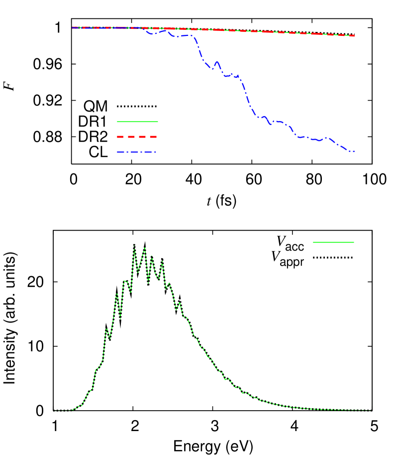
Figure 1: Fidelity decay (top) and spectrum change (bottom) for $D_{e,\text{CO}}^{\prime}=D_{e,\text{CO}}+0.02\operatorname{eV}=11.26\operatorname{eV}$.

Figure 2: Fidelity decay (top) and spectrum change (bottom) for $R_{e,\text{CO}}^{\prime}=R_{e,\text{CO}}+0.02\,a_{0}=2.15\,a_{0}$. Notation as in Fig. 1.

One could object that since DR is an intrinsically SC approximation, it might suffice to estimate fidelity classically. We explored this idea by comparing quantum fidelity with its classical (CL) analog, called classical fidelity Prosen and Žnidarič (2002), defined in our case by

$$F_{\text{CL}}(t):=h^{d}\int dx\,\rho_{\text{CL,acc}}^{t}(x)\rho_{\text{CL,appr}}^{t}(x),$$ (6)

where $\rho_{\text{CL}}^{t}$ is the CL phase-space density evolved with the indicated potential to time $t$. For initial Gaussian wave packets, $\rho_{\text{CL}}^{0}=\rho_{\text{W}}^{0}$. Unlike DR, classical fidelity does not include any dynamical quantum effects, and below we show that indeed $F_{\text{CL}}$ gives much worse results.

To show the feasibility of our method, we have applied it to the photodissociation dynamics of a collinear carbon dioxide molecule, a model that had been studied extensively by both quantum-dynamical Kulander and Light (1980); Schinke and Engel (1990) and SC methods VanVoorhis and Heller (2002). Invoking the Franck-Condon principle, photodissociation process is described by the quantum dynamics of the initial state (vibrational ground state of the electronic ground state PES) on the dissociative excited PES. One can obtain the photodissociation spectrum simply by taking the Fourier transform of the autocorrelation function $C(t):=\langle\psi(0)|\psi(t)\rangle$. In future applications, one will not be able to find $\psi_{\text{acc}}(t)$ and $f_{\text{QM}}(t)$ due to the tremendous computational expense. Here, in order to demonstrate the accuracy of the method, we want to compare $f_{\text{DR}}(t)$ with $f_{\text{QM}}(t)$ and so we define $V_{\text{acc}}:=V_{\text{LEPS}}$ to be the analytical LEPS potential for CO₂ Sato (1955); Kulander and Light (1980) and $V_{\text{appr}}:=V_{\text{LEPS}}^{\prime}$ to be the LEPS potential with one of the parameters perturbed. Specifically, we change either the equilibrium bond length $R_{e,\text{CO}}$ or the bond dissociation energy $D_{e,\text{CO}}$ of the CO bond. We imagine that we would like to obtain a spectrum corresponding to $V_{\text{acc}}$ but can only afford quantum dynamics on $V_{\text{appr}}$. By estimating quantum fidelity amplitude $f_{\text{QM}}$ by $f_{\text{DR}}$, we can determine whether we can trust the spectrum computed using quantum dynamics on $V_{\text{appr}}$. From another perspective, we can use $f_{\text{DR}}$ to evaluate how errors in experimental values of $R_{e,\text{CO}}$ and $D_{e,\text{CO}}$ affect the computed spectrum.

Figure 1 shows an example where $V_{\text{LEPS}}^{\prime}$ has a perturbed bond dissociation energy, $D_{e,\text{CO}}^{\prime}=D_{e,\text{CO}}+0.02\operatorname{eV}=11.26\operatorname{eV}$. The figure shows that three approaches to compute fidelity (QM, DR1, DR2) give very similar results. This turns out to be a small perturbation since fidelity remains close to unity, $F_{\text{QM}}\geq 0.99$. Therefore we should be able to trust the spectrum computed using $\psi_{\text{appr}}(t)$. This is justified in the bottom panel where spectra corresponding to $V_{\text{acc}}$ and $V_{\text{appr}}$ prove to be almost identical . Unlike DR, classical fidelity (CL) decays much faster than its quantum analog. Judging by $F_{\text{CL}}$ only, one would conclude incorrectly that the spectrum computed using $V_{\text{appr}}$ should not be trusted. Partially constructive interference, captured by DR, prevents quantum fidelity from decaying with the fast rate of classical fidelity decay.

Figure 2 shows an example where $V_{\text{LEPS}}^{\prime}$ has a perturbed equilibrium bond length, $R_{e,\text{CO}}^{\prime}=R_{e,\text{CO}}+0.02\,a_{0}=2.15\,a_{0}$. The figure shows that $F_{\text{DR}}$ agrees with $F_{\text{QM}}$ and even reproduces detailed oscillations of quantum fidelity. This turns out to be a large perturbation since fidelity falls below the value of $0.5$. We therefore expect the spectrum computed using $\psi_{\text{appr}}(t)$ to differ significantly from the “true” spectrum computed using $\psi_{\text{acc}}(t)$. Indeed, the bottom panel shows that the spectrum of $V_{\text{appr}}$ is shifted and has different peak intensities than the spectrum of $V_{\text{acc}}$. Figure 2 also shows that for large $\Delta V$, classical fidelity starts to behave similarly to quantum fidelity, but is still much worse than DR.

All calculations were performed for $600$ time steps of $0.16\operatorname{fs}$ each. Converged quantum calculations required $n=1024$ points to discretize each CO bond length from $0$ to $20\,a_{0}\approx 10.6\operatorname{\mathring{A}}$, altogether using a $1024\times 1024$ grid to represent the PES and the wave function. The DR calculation converged fully with $n_{\text{paths}}=512$ trajectories (shown in Figs. 1 and 2), but a much smaller value, $n_{\text{paths}}=64$, already gives very accurate results sufficient for our application (not shown). Both figures show fidelity $F$, rather than fidelity amplitude $f$ which is a complex number containing more information. If $F\ll 1$, clearly our approximate dynamics is not sufficient. However, if $F\approx 1$, the spectrum could still be affected by a time-dependent phase of $f$. In such cases one should also examine fidelity amplitude.

Our fidelity calculation for photodissociation of CO₂ is to our knowledge the first fidelity calculation for a realistic chemical system and it is reassuring that DR remains valid Gorin et al. (2006). Clearly, in chemical physics one is interested in systems with many more than two DOF. However, already in the simple CO₂ system, the DR calculation of fidelity was more than $100$ times faster than the exact quantum calculation. We expect that in larger systems, much larger speedups could be achieved.

The information required in a DR calculation is similar to information needed in molecular dynamics (MD). Implementation of DR into any MD code would require a single addition: calculation of the action $\Delta S$. But there is an important difference between DR and MD: in DR, nuclear quantum effects are included at least approximately, whereas in MD, even if ab initio electronic potential is used, they are completely lost. This can be clearly seen in Figs. 1 and 2 where $F_{\text{DR}}\approx F_{\text{QM}}\neq F_{\text{CL}}$ since $F_{\text{CL}}$ is basically a MD calculation of fidelity. With little effort, MD codes that currently compute only classical nuclear dynamics, could be used for evaluating accuracy of quantum dynamics on the same PES.

The method was designed with the goal of determining the accuracy of quantum dynamics on an approximate PES compared to the exact dynamics. As mentioned above, we do not know $V_{\text{exact}}$ and instead must use $V_{\text{acc}}$. We predict that if one could show $V_{\text{acc}}$ to be much closer to $V_{\text{exact}}$ than to $V_{\text{appr}}$, our estimate of fidelity would predict the accuracy compared to the exact dynamics, and not just compared to the dynamics on $V_{\text{acc}}$.

The DR approach is applicable to other types of perturbations of the Hamiltonian than discrepancies in the PES. For example, DR could be used to evaluate how laser pulse noise affects quantum control Li et al. (2002) or how perturbations affect quantum computation. To conclude, we do not claim to have found a fast way to do quantum dynamics on an accurate ab initio potential. Instead we have found a promising method to estimate the accuracy of quantum dynamics on an approximate potential.

This research was supported by the startup funding provided by École Polytechnique Fédérale de Lausanne. We thank Tomáš Zimmermann for useful discussions.

References

- Clary (2008) D. C. Clary, Science 321, 789 (2008).
- Makri (1999) N. Makri, Ann. Rev. Phys. Chem. 50, 167 (1999).
- Miller (2005) W. H. Miller, Proc. Natl. Acad. Sci. 102, 6660 (2005).
- Rabitz (1987) H. Rabitz, Chem. Rev. 87, 101 (1987).
- Peres (1984) A. Peres, Phys. Rev. A 30, 1610 (1984).
- Gorin et al. (2006) T. Gorin, T. Prosen, T. H. Seligman, and M. Žnidarič, Phys. Rep. 435, 33 (2006).
- Vaníček (2004a) J. Vaníček, Phys. Rev. E 70, 055201(R) (2004a).
- Vaníček (2006) J. Vaníček, Phys. Rev. E 73, 046204 (2006).
- Cerruti and Tomsovic (2002) N. R. Cerruti and S. Tomsovic, Phys. Rev. Lett. 88, 054103 (2002).
- Vaníček and Heller (2003) J. Vaníček and E. J. Heller, Phys. Rev. E 68, 056208 (2003).
- Vaníček (2004b) J. Vaníček (2004b), preprint quant-ph/0410205.
- Vaníček et al. (2009) J. Vaníček, C. Mollica, T. Prosen, and W. Strunz (2009), not published.
- Feit et al. (1982) M. D. Feit, J. J. A. Fleck, and A. Steiger, J. Chem. Phys. 47, 412 (1982).
- Prosen and Žnidarič (2002) T. Prosen and M. Žnidarič, J. Phys. A 35, 1455 (2002).
- Kulander and Light (1980) K. C. Kulander and J. C. Light, J. Chem. Phys. 73, 4337 (1980).
- Schinke and Engel (1990) R. Schinke and V. Engel, J. Chem. Phys. 93, 3252 (1990).
- VanVoorhis and Heller (2002) T. VanVoorhis and E. J. Heller, Phys. Rev. A 66, 050501(R) (2002).
- Sato (1955) S. Sato, J. Chem. Phys. 23, 592 (1955).
- Li et al. (2002) B. Li, G. Turinici, V. Ramakrishna, and H. Rabitz, J. Phys. Chem. B 106, 8125 (2002).