Method for the determination of the three-dimensional structure of ultrashort relativistic electron bunches

Abstract

We describe a novel technique to characterize ultrashort electron bunches in X-ray Free-Electron Lasers. Namely, we propose to use coherent Optical Transition Radiation to measure three-dimensional (3D) electron density distributions. Our method relies on the combination of two known diagnostics setups, an Optical Replica Synthesizer (ORS) and an Optical Transition Radiation (OTR) imager. Electron bunches are modulated at optical wavelengths in the ORS setup. When these electron bunches pass through a metal foil target, coherent radiation pulses of tens MW power are generated. It is thereafter possible to exploit advantages of coherent imaging techniques, such as direct imaging, diffractive imaging, Fourier holography and their combinations. The proposed method opens up the possibility of real-time, wavelength-limited, single-shot 3D imaging of an ultrashort electron bunch.

DEUTSCHES ELEKTRONEN-SYNCHROTRON

in der HELMHOLTZ-GEMEINSCHAFT

DESY 09-069

May 2009

Method for the determination of the three-dimensional structure of ultrashort relativistic electron bunches

Gianluca Geloni, Petr Ilinski, Evgeni Saldin, Evgeni Schneidmiller and Mikhail Yurkov

Deutsches Elektronen-Synchrotron DESY, Hamburg ISSN 0418-9833 NOTKESTRASSE 85 - 22607 HAMBURG

1 Introduction

Three X-ray Free-Electron Lasers (XFELs), LCLS LCLS , SCSS SCSS , and the European XFEL XFEL are currently under commissioning or under construction. These machines are based on the Self-Amplified Spontaneous Emission (SASE) process KOND -PELL and will be operating with electron bunch durations of less than $100$ fs.

Operational success of XFELs will be related to the ability of monitoring the spatio-temporal structure of these sub-$100$ fs electron bunches as they travel along the XFEL structure. However, the femtosecond time-scale is beyond the scale of standard electronic display instrumentation. Therefore, the development of methods for characterizing such short electron bunches both in the longitudinal and in the transverse directions is a high-priority task, which is very challenging.

A method for peak-current shape measurements of ultrashort electron bunches was proposed in ORSS . It uses the undulator-based Optical Replica Synthesizer (ORS), together with the ultrashort laser pulse shape measurement technique called Frequency-Resolved Optical Gating (FROG) FROG . It was demonstrated in ORSS that the peak-current profile for a single, ultrashort electron bunch could be determined with a resolution of a few femtoseconds. The ORS method is currently being tested at the Free-electron laser in Hamburg (FLASH) ANG2 .

Recently, feasibility studies for integrating the ORS diagnostics setup with a timing scheme for pump-probe experiments and with a scheme for output-power stabilization of an X-ray SASE FEL were presented in TIME and STAB . Both schemes rely on an external optical laser to modulate the energy of an electron bunch in a short undulator. Such energy-modulation is subsequently converted into density modulation by means of a dispersive section. Since the ORS setup already includes seed laser, energy modulator undulator and dispersion section, it is the most natural option to be considered in the implementation of both timing and stabilization schemes.

In this paper we present a feasibility study for integrating the ORS setup with a high-resolution electron bunch imager based on coherent Optical Transition Radiation (OTR).

Electron bunch imagers based on incoherent OTR constitute the main device presently available for the characterization of an ultrashort electron bunch in the transverse direction. They work by measuring the transverse intensity distribution. However, since no fast enough detector is presently available, the image is actually integrated over the duration of the electron bunch. Therefore, incoherent OTR imagers fail to measure the temporal dependence of the charge density distribution within the bunch. For these reasons, the use of standard incoherent OTR imagers is limited to transverse electron-beam diagnostics, to measure e.g. the projected transverse emittance of electrons.

However, it is primarily the emittance of electrons in short axial slices, which determines the performance of an XFEL. There is, therefore, a compelling need for the development of electron diagnostics capable of measuring three-dimensional (3D) ultrashort electron bunch structures with micron-level resolution.

The main advantages of coherent OTR imaging with respect to the usual incoherent OTR imaging is in the coherence of the radiation pulse, and in the high photon flux. Exploitation of these advantages lead to applications of coherent OTR imaging that are not confined to diagnostics of the transverse distribution of electrons. The novel diagnostic techniques described here can indeed be used to determine the 3D distribution of electrons in a ultrashort single bunch. In combination with multi-shot measurements and quadrupole scans, they can also be used to determine the electron bunch slice emittance.

The possibility of single-shot, 3D imaging of electron bunches with microscale resolution makes coherent OTR imaging an ideal on-line tool for aligning the bunch formation system at XFELs.

Future XFEL operation will set tight tolerances on electron bunch trajectories. They need to be carefully monitored along the full-length of the machine. In order to ensure SASE lasing at X-ray wavelengths, a very high orbit accuracy of a few microns has to be ensured in the $200$ m long undulator. The resolution of incoherent OTR imagers is not adequate to characterize the position of the center of gravity of an electron bunch with such accuracy. Our studies show that coherent OTR imaging can be utilized as an effective tool for measuring the absolute position of the electron bunch with the required micron accuracy.

Finally, the improvement of bunch-imaging techniques up to the microscale level does not only yield a powerful diagnostic tool, but opens up new possibilities in XFEL technology as well.

A pioneering experiment for integrating the ORS setup with a coherent OTR imager was performed at FLASH. The energy of the coherent OTR pulse was measured as a function of the position of a relatively short seed laser pulse along the (long) bunch, i.e. the slice peak-current was measured. First attempts to extract information about the correlation between longitudinal and transverse distribution also took place. These results, which should be considered as first steps into a novel direction of electron-beam diagnostics, are reported in ANGE .

In this work, we illustrate the potential of the proposed coherent OTR imager scheme for the case of the European XFEL XFEL . We show that it naturally fits into the project. Technical realization will be straightforward and cost-effective, since it is essentially based on technical components (ORS, OTR diagnostics stations), which are already included in the design of the European XFEL. In our analysis we considered the baseline parameters, so that our scheme can be implemented at the very first stage of operation of the European XFEL facility. However, the applicability of our method is not restricted to the European XFEL setup. Other projects, e.g. LCLS or SCSS LCLS , SCSS may benefit from this work as well.

Our paper is organized as follows. In the next Sections 2, 3 and 4 we introduce basic concepts and important details pertaining the Optical Replica method, the coherent OTR generation and the image formation of a modulated electron bunch.

In Section 5 we analyze a coherent OTR imaging setup, the so called $4f$ filtering architecture, which is relatively simple to implement experimentally. We demonstrate that such setup can be used to characterize electron density profiles on the microscale level. Such resolution level can be reached by taking advantage of a number of options, including e.g. spatial filtering in the Fourier plane and radial-to-linear polarization conversion, which make coherent OTR imaging more accurate.

Diffractive imaging is one of the most promising techniques for microscale imaging of electron bunches, when a detector records the Fraunhofer diffraction pattern radiated by the electron bunch. Subsequently, an image can be reconstructed with the help of a phase retrieval algorithm. This method reduces the requirements on the optical hardware by increasing the sophistication in the post-processing of the data collected by the system. Besides, a diffractive imaging setup has the same ultimate resolution of the $4f$ coherent imaging setup. This extremely simple method is discussed for two versions, with and without the use of lenses, in Section 6.

Fourier-Transform Holography (FTH) is analyzed as another promising imaging method in Section 7. FTH is a non-iterative imaging technique, so the image can be reconstructed in a single step deterministic computation. This is achieved by placing a coherent point source at an appropriate distance from the object and having the object field interfering with the reference wave produced by this point source, detecting the interference pattern in the Fourier plane. For optical applications, the resolution of holographic techniques is not limited by size and quality of the point-like source. With the help of modern lithographic methods it is not difficult to produce a pinhole, unresolved at optical wavelengths, and let sufficiently bright radiation through it. The fast, unambiguous and direct reconstruction achieved in FTH is attractive for coherent OTR imaging of electron bunches. Moreover, FTH may also be used to generate a low-resolution image of the bunch to support diffractive imaging techniques. In this case, multiple references can be added to the FTH setup in order to increase the a-priori information available.

One of the main unsolved problems in XFEL electron bunch diagnostics is the characterization of bunches that have significant distortions in transverse phase space, e.g. bunches whose transverse phase-space ellipse varies along the beam itself. In an RF photoinjector with perfectly working emittance compensation technique, the electron beam transverse profile is axis-symmetric, and the Twiss parameters are equal in all slices (excluding the emittance, which varies). For a real beam, the variation in the space charge forces can be significant and cannot be properly compensated with a solenoid emittance compensation scheme. In addition, Coherent Synchrotron Radiation (CSR) related effects in bunch compressors can lead to further deviations from the axis-symmetric model. The knowledge of the variation of the phase-space ellipse along the bunch at the output of the bunch formation system could provide significant information about the physical mechanisms responsible for the generation of ultrashort bunches in XFELs. If the 3D structure of electron bunches could be provided (even as the result of a multi-shot measurement), a quadrupole-scan (which is a multi-shot measurement method too) could be used to provide phase-space density distribution measurements. Twiss parameters in each slice could be reconstructed in this way.

As mentioned above, the applications of coherent OTR imaging are not confined to diagnostics of the transverse distribution of electrons projected along the longitudinal axis.

Simple extensions of our proposed diagnostic techniques allow for the characterization of the 3D structure of electron bunches with a multi-shot measurement. Our approach, described in Section 6, involves a combination of real and reciprocal space imaging spectrometers. Both imaging setups use frequency filters to obtain the spectral data of the image. When the filter bandpass is changed, successive images are recorded at different wavelengths. This process is repeated, wavelength by wavelength, until the entire spatial spectral data is built up slice by slice. The result is the simultaneous knowledge of two ”3D cubes” of spectral data, one in the real space $(\Delta\lambda,\Delta x,\Delta y)$ and the other in the reciprocal space $(\Delta\lambda,\Delta\omega_{x},\Delta\omega_{y})$, having indicated with $\omega_{x,y}$ the spatial frequencies relative to the $x$ and $y$ axis. Application of e.g. the Gerchberg-Saxton algorithm GERC , which is the first practical iterative algorithm to have been developed for solving the Fourier-phase-retrieval problem, allows one to retrieve the spatio-temporal electron-bunch structure.

In Section 6 we also show how the determination of the projections of the cube of data in reciprocal space onto specific planes of interest is sufficient to reconstruct the electron-bunch structure, even without knowledge about the cube of spectral data in real space. The advantage of this method is that it requires no reference pulse shorter than the electron bunch (i.e. no synchronization). In other words, the optical replica pulse can be measured in the 3D Fourier domain. We name this novel method Frequency-Resolved Optical Diffractive Imaging (FRODI).

FRODI is further developed in Section 6 from a multi-shot to a single-shot technique to measure the 3D structure of a single electron bunch. This is accomplished by splitting the beam and simultaneously measuring orthogonal $(x,t)$, $(y,t)$ and $(x,y)$ projections. The entire traces can be recorded by three detectors, and used to reconstruct the desired 3D electron-bunch structure.

While FROG requires the use of nonlinear-optical process, FRODI is a linear-optical method, and linear-optical processes do not require intense pulses. Here we discuss about measurements of complicated pulses in three dimensions, and it is interesting to compare FRODI with the well-known FROG technique, which can measure complicated pulses in one dimension (1D). As was reported in FROG concerning measurements of temporal structures in optical pulses: ”It can be shown that linear-optical methods cannot completely measure ultrashort pulses”. Quite counter-intuitively, the measurement of 3D structures of optical pulses in time and space is simpler than the measurement of temporal 1D structures alone. However, in analogy with this fact, it is well-known that the two-dimensional (2D) phase retrieval problem is solvable, unlike the 1D one. To detect the temporal structure of optical pulses, FROG requires the use of a nonlinear optical process, which allows to extend the 1D reconstruction problem to a 2D reconstruction problem. This involves an artificial 2D Fourier domain. Unlike it, FRODI transforms the problem of measurement of 3D structures in time and space into measurements of the more natural 3D spatial-frequency and temporal-frequency domains. No prior information about the electron bunch structure is necessary to reconstruct the electron bunch density distribution from the experimental traces.

Our 3D imaging technique FRODI turns out to be a relatively simple solution to a very complicated problem. For the 3D (spatio-temporal) electric field of optical replica pulses produced by optically-modulated electron bunches with spatio-temporal distortions, different spatial frequencies are related to different temporal spectra (i.e. spatial frequency and temporal frequency are coupled).

Multi-shot and single-shot techniques for the characterization of the electron bunch can also be based on FTH setups. A new multi-shot technique for 3D imaging of the electron bunch based on frequency gated FTH is discussed in Section 7. In the same Section 7 we also consider spatio-temporal FTH techniques. An extension of the method opens up the possibility for single-shot 3D imaging of ultrashort electron bunches.

Time-gated FTH is the next class of techniques discussed in Section 7. The principle of this method is straightforward. A hologram records information about the object only when it is illuminated simultaneously by a coherent reference wave. Then, when a short reference is used, the hologram is equivalent to a time-gated viewing system ABRA . We propose a method based on time-gated FTH with multiple reference sources capable of characterizing the spatio-temporal structure of individual electron bunches. Multiple, ultrashort (about $10$ fs) reference pulses are generated with a varying time-delay, so that several two-dimensional images (frames) of the electron bunch at different position inside the bunch can be reconstructed from a single holographic pattern. We call this technique Holography Optical Time Resolved Imaging (HOTRI).

We conclude our work in Section 9.

2 Optical replica setup

2.1 Optical replica pulse generation

We propose to create a coherent pulse of optical radiation by first modulating the electron bunch at a given optical wavelength and, second, by letting it pass through a metal foil target, thus producing coherent Optical Transition Radiation (OTR) at the modulation wavelength. The radiation pulse should be produced in such a way as to constitute an exact replica of the electron bunch. Such optical replica can be used for the determination of the 3D structure of electron bunches. Although other projects may benefit from our study too, throughout this paper we will mainly refer to parameters and design of the European XFEL.

In order to produce the optical replica we need to modulate the electron bunch at a fixed optical wavelength. One may take advantage of an Optical Replica Synthesizer (ORS) modulator ORSS , which we suppose to be installed after the BC2 bunch compressor chicane. A basic scheme to generate coherent OTR is shown in Fig. 1.

A relatively long laser pulse serves as a seed for the modulator, consisting of a short undulator and a dispersion section. The central area of the laser pulse should overlap with the electron pulse. In order to ensure simple synchronization, the duration of the laser pulse should be much longer than the electron pulse time jitter, which is estimated to be of the order of $100$ fs. Foreseen parameters of the seed laser are: wavelength $\lambda_{m}=800$ nm, energy in the laser pulse $1$ mJ and pulse duration (FWHM) $1$ ps. The laser beam is focused onto the electron bunch in a short (the number of periods is $N_{w}=5$) modulator undulator resonant at the optical wavelength of $800$ nm. Optimal conditions of focusing are met by positioning the laser beam waist into the center of the modulator undulator, with a Rayleigh length of the laser beam equal to the undulator length. Since the electron betatron function $\beta$, the undulator length $L_{w}$ and the Rayleigh length of the laser beam are of the same magnitude, the size of the laser beam waist turns out to be about $20$ times larger than the electron beam size. As a consequence, we can approximate the laser beam with a plane wave when discussing about the modulation of the electron bunch.

The seed laser pulse interacts with the electron beam in the modulator undulator and produces an amplitude of the energy modulation in the electron bunch of about $500$ keV. Subsequently, the electron bunch passes through the dispersion section (with momentum compaction factor $R_{56}\simeq 50\mu$m), where the energy modulation is converted into density modulation at the laser wavelength. The electron bunch density modulation reaches an amplitude of about $10\%$.

Finally, the modulated electron bunch travels through the OTR screen. A powerful burst of OTR is emitted, which contains coherent and incoherent parts. The coherent OTR has much greater number of photons (up to $10^{13}$ i.e. $1\mu$J per pulse, as we will see), and can be used for diagnostic purposes. A quantitative treatment for coherent OTR is presented in Section 3. The way we can take advantage of coherent OTR properties is discussed in the following Sections.

Figure 1: Schematic diagram of the coherent imager. The working principle is based on the optical modulation of the electron bunch and on emission of coherent OTR radiation from the metallic mirror.

It should be mentioned that OTR screens can be positioned at various locations down the electron beam line where electrons have substantially different energies. In the case of the European XFEL XFEL , the electron energy varies from $2$ GeV (second bunch compression chicane) up to $17.5$ GeV at the undulator entrance. For other machines, these parameters differ. In the case of LCLS LCLS , energies will range from about $4.5$ GeV to $13.6$ GeV.

Reference ORSS includes a discussion about how to avoid the influence of self-interaction effects in the ORS setup, when the radiator is placed just behind the modulator. This case is practically realized, for example, when we want to use a 3D OTR imager to align the bunch formation system, and the OTR station is placed just after the ORS setup behind the second bunch compressor at $2$ GeV. The situation changes when the OTR imager is placed behind the main XFEL accelerator at $17.5$ GeV, and the distance between ORS modular and OTR imager is in the kilometer scale. In Section 2.3 we will present ideas how to avoid self-interaction effects in the high-energy case. When, instead, the ORS setup and the OTR imager are placed just behind the bunch compression system, it sufficient to use the ideas introduced in ORSS .

2.2 Optical modulator

In order to use the coherent OTR burst for diagnostic purposes, one has to ensure that an optical replica of the electron bunch is actually produced. In fact, the electron bunch density modulation can be perturbed by collective fields. It is therefore important to consider collective interactions (radiation and space-charge fields) influencing the operation of the Optical Replica modulator, to ensure that longitudinal dynamics in the Optical Replica modulator is governed by single-particle effects, independently of the presence of other particles. In particular, our method for electron-beam structure measurements is based on the assumption that the electron bunch density modulation does not appreciably change due to longitudinal space-charge (LSC) interactions, i.e. plasma oscillations, as the beam propagates through the setup behind the Optical Replica modulator, up to the OTR station. Thus, the passage of the modulated electron bunch through the setup must be studied.

Even when self-interactions are negligible, distortions can be introduced due to nonuniform local energy spread within the electron bunch.

Let us first consider under which conditions on the Optical Replica modulator, the energy-spread effects are negligible. The way the electron bunch is modulated in the modulator is quantitatively described in e.g. CZON . The current $I$ at the exit of the dispersion section is found to be a composition of harmonics of the modulation frequency $\omega_{m}$:

$$I = I_{0}+2I_{0}\sum_{n=1}^{\infty}\exp\left[-\frac{n^{2}}{2}\langle(\Delta\mathcal{E})^{2}\rangle\left(\frac{\omega_{m}R_{56}}{c\mathcal{E}_{0}}\right)^{2}\right]J_{n}\left(nP_{0}\frac{\omega_{m}R_{56}}{c\mathcal{E}_{0}}\right)$$ (4)

$$\times\cos\left[n\omega_{m}\left(\frac{z}{v_{z}}-t\right)\right]~{},$$

where $P_{0}=500$ keV is the initial energy modulation, $\mathcal{E}_{0}$ is the nominal electron energy, $\sqrt{\langle(\Delta\mathcal{E})^{2}\rangle}$ is the local energy spread of electrons, $z$ is the longitudinal coordinate, $v_{z}$ is the longitudinal velocity of electrons and $t$ is the time. Moreover $J_{n}$ indicates the Bessel function of the first kind of order $n$ and, as before, $R_{56}$ is the momentum compaction factor. Note that the current is, in general a function of the time, i.e. $I_{0}=I_{0}(t)$. However, throughout this paper we will make use of the adiabatic approximation, because the electron bunch is much longer than the modulation wavelength. As a result, we can consider $I_{0}$ as a local parameter, and discuss about local amplitude and phase of the density modulation.

As one can see from Eq. (4), the microbunching depends on the choice of the dispersion section strength. In fact, neglecting the exponential suppression factor in $\sqrt{\langle(\Delta\mathcal{E})^{2}\rangle}$, the expression for the fundamental component of the bunched beam current is $I_{1}\propto 2I_{0}J_{1}(X)\sim I_{0}X$ for $X\ll 1$, where $X=P_{0}{R_{56}}/({\lambdabar_{m}\mathcal{E}_{0}})$, with $\lambdabar_{m}=c/\omega_{m}$, is a small dimensionless quantity known as the bunching parameter.

One might think that all we have to do is to get the microbunching amplitude to a maximum by increasing the $R_{56}$ of the dispersion section, thus increasing the output power. In fact, it is possible to build a dispersion section with a large $R_{56}$ function. However, one of the main problems in the modulator operation is preventing the spread of microbunching due to local energy spread in the electron bunch. In other words, for effective operation, the value of the suppression factor in the exponential factor in Eq. (4) should be close to unity ORSS .

The energy spread is not constant along the electron bunch. For example, the energy-spread distribution in the case of the European XFEL is given in Fig. 2, reproduced from XFEL . The maximal energy spread level is about $1$ MeV. Substituting numbers into the argument of the exponential function (remember that the chicane of the modulator has dispersion strength $R_{56}\simeq 50~{}\mu$m) one finds that, for the first harmonic ($n=1$) the exponential factor is about unity ($\simeq 0.998$) even for $\mathcal{E}_{0}=2$ GeV, which is the minimal energy considered. Moreover, the second harmonic ($n=2$) of the modulation is suppressed by an order of magnitude with respect to the first, due to the Bessel $J_{2}$ factor.

As a result, in our case we can approximate Eq. (4) with

$$I=I_{0}+I_{0}\cdot\frac{P_{0}R_{56}}{\lambdabar_{m}\mathcal{E}_{0}}\cos\left[\omega_{m}\left(\frac{z}{v_{z}}-t\right)\right]~{},$$ (5)

which ensures that the bunching is uniform along the beam. Calling $\psi=\omega_{m}[z/v_{z}(\gamma_{0})-t]$ the modulation phase, the current can be expressed as $I=I_{0}[1+a\cos(\psi)]$, where $a$ is the amplitude of our small ($|a|\ll 1$) density modulation, taken with its own sign.

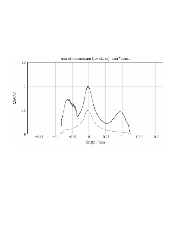
Figure 2: Energy spread profile (rms, solid line) at the entrance of the SASE undulator (after XFEL TDR) XFEL ).

Let us now discuss distortions due to self-interaction effects. Concerning the induced bunching inside the modulator undulator, perturbations due to collective effects are minimized up to a negligible level by using a small number of periods ($N_{w}=5$). This optimization is also important in order to increase the replica resolution and minimize slippage effects ($N_{w}\lambda/c\ll\sigma_{T}$, $\sigma_{T}$ being the electron bunch duration).

Concerning the effect of LSC interactions, one needs a more detailed analysis. The propagation of the induced electron bunch density modulation through the setup is a problem involving self-interactions. If the OTR station is placed at a short distance (say, a few meters) from the modulator, e.g. to align the bunch formation system, plasma oscillations play no important effect, as it will be clear after reading the following analysis. However, the situation changes if one wants to characterize the electron beam after the linac, to monitor the electron bunch properties along the machine and, in particular, to monitor electron trajectories in the undulator. In fact, as the bunch progresses through the linac, the modulation of the bunch density produces energy modulation due to the longitudinal impedance caused by space-charge fields. This process is complicated by the fact that, due to the presence of energy and density modulation, plasma oscillations can develop.

As a result, the initial energy and density modulation of the electron bunch will be modified by the passage through the setup. In order to study the feasibility of our scheme one needs to estimate what modifications take place. For a given facility, OTR screens positioned at a higher electron energy translate into a longer distance between modulator and OTR screen and, thus, into a stronger LSC influence. However, the evolution of plasma oscillations tends to slow down as the energy increases. This means that LCLS is less affected than the European XFEL, because the last magnetic bunch compressor at LCLS is positioned at higher energy ($4.5$ GeV compared to the $2$ GeV of the European XFEL).

Figure 3: Schematic diagram of the European XFEL setup from BC2 through SASE1.

2.3 Distortions of the optical microbunching downstream the main accelerator

Let us consider the European XFEL case, where self-interactions are more important (see Fig. 3). Proceeding as in TIME we find that energy and density modulation along the accelerator are linked by the following system of differential equations:

$$\frac{da}{dz}=\frac{1}{\lambdabar}\frac{\Delta\gamma(z)}{(\gamma_{0}+gz)^{3}}~{},$$ (6)

$$\frac{d(\Delta\gamma)}{dz}\simeq-\frac{a(z)}{\lambdabar(\gamma_{0}+gz)^{2}}\frac{I_{0}}{I_{A}}{\exp\left[\frac{\epsilon_{n}\beta}{(\gamma_{0}+gz)^{3}\lambdabar^{2}}\right]~{}\Gamma\left[0,\frac{\epsilon_{n}\beta}{(\gamma_{0}+gz)^{3}\lambdabar^{2}}\right]}~{},$$ (7)

where we assumed that $\gamma(z)=\gamma_{0}+gz$, with $g$ the acceleration gradient and $\gamma_{0}\simeq 4\cdot 10^{3}$. The density modulation $a$ has been defined above, and the energy modulation is given by $\Delta\gamma\sin(\psi)$. Here $I_{A}\simeq 17$ kA is the Alfven current, $\epsilon_{n}$ is the normalized emittance, $\beta$ is the average betatron function and $\Gamma(\alpha,\beta)$ is the incomplete gamma function.

Usually, calculating self-interaction effects is rather challenging. In our case, however, we used the straightforward 1D model in Eq. (6) and Eq. (7). Remarkably, such model is not a rough approximation of reality, but it rather constitutes a quantitative approach. In fact, in our case study we deal with a very particular range of parameters where four asymptotic limits can be simultaneously exploited. First, retardation effects can be neglected due to a small current $I\ll\gamma I_{A}$, and to the adiabatic acceleration limit $\lambdabar(d\gamma^{2}/dz)\ll 1$. Second, the adiabatic approximation applies, i.e. $\omega\sigma_{T}\gg 1$. Third, a pencil beam (1D) approximation is valid because $\sigma_{r}\ll\gamma\lambdabar$, with $\sigma_{r}$ the bunch transverse dimension. Finally, fourth, we can neglect the interaction of space-charge fields with material structures because $\gamma\lambdabar\ll b$, $b$ being the characteristic dimension of the vacuum chamber. As a result, when dealing with an XFEL setup and discussing about optical microbunching, we have a unique situation. If any of the conditions above ceases to be valid, the model in Eq. (6) and Eq. (7) ceases to be valid too, as it would be the case e.g. for calculations of impedance at lower frequencies.

Figure 4: Evolution of the electron bunch density modulation as a function of the distance from the modulator.

Let us then use Eq. (6) and Eq. (7) assuming an average betatron function of about $\beta=25$ m along the main accelerator and a normalized emittance $\epsilon_{n}=1.4$ mm$\cdot$mrad (see XFEL ). We set the acceleration length in the main linac equal to $d_{a}\simeq 1220$ m. The undulator does not follow immediately the main linac, as it can be seen from Fig. 3. For example, the SASE $1$ undulator is preceded by a $290$ meters long straight section and by a collimation system, which is $215$ meters long. According to XFEL , the compaction factor of the collimator can be set to any value from $R^{(c)}_{56}=-2~{}$mm to $R^{(c)}_{56}=2~{}$mm, with possibility of fine tuning (not in real time) of about $\pm 100~{}\mu$m.

In practical situations, one is interested in inserting OTR screens just after the bunch compression chicane (at $2$ GeV) or along the undulator at $17.5$ GeV. The situation where the influence of self-interactions is most important is obviously at $17.5$ GeV along the undulator. As shown in OURX , the longitudinal Lorentz factor $\gamma_{z}=\gamma/\sqrt{1+K^{2}/2}$ should be used in the undulator instead of $\gamma$. Since $K=3.3$, $\gamma^{2}$ and $\gamma_{z}^{2}$ differ of about an order of magnitude, hence a different influence of the LSC in the undulator compared to the straight section. In the undulator, Eq. (6) and Eq. (7) are modified to

$$\frac{da}{dz}=\frac{1}{\lambdabar}\frac{\Delta\gamma}{\gamma\gamma_{z}^{2}}~{},~{}~{}~{}~{}~{}~{}\frac{d\Delta\gamma}{dz}\simeq-\frac{a(z)}{\lambdabar\gamma_{z}^{2}}\frac{I_{0}}{I_{A}}{\exp\left[\frac{\epsilon_{n}\beta}{\lambdabar^{2}\gamma\gamma_{z}^{2}}\right]~{}\Gamma\left[0,\frac{\epsilon_{n}\beta}{\lambdabar^{2}\gamma\gamma_{z}^{2}}\right]}~{},$$ (8)

where now $\gamma=3.5\cdot 10^{4}$. Even for a simple case study where we set $R^{(c)}_{56}=0$, numerical analysis shows that our initial conditions $a_{i}\simeq 0.1$ and $(\Delta\gamma)_{i}\simeq 1$ yield an unwanted evolution of $a(z)$ as summarized in Fig. 4.

Figure 5: Installation of a small dispersive element (chicane) after the collimation system will allow to compensate positional-dependent variations of the electron bunch density modulation level.

As one may see, the electron bunch density modulation is diminished by at most $\Delta a/a_{i}=25\%$ at highest energies and at the end of the undulator. This constitutes a detrimental effect concerning our imaging techniques. In fact, we calculated $a(z)$ assuming a fixed peak-current $I_{0}=5$ kA. However, the peak-current along the bunch is not constant, and from Eq. (6) and Eq. (7) follows that the modulation level varies along the bunch in a complicated way depending on the variation of the peak-current level. This effect is unwanted. In fact, different parts of the electron bunch should be given the right weight as concerns their contribution to radiation emission, meaning that the (absolute) charge modulation in each point of the electron bunch should be proportional to the charge density distribution of the unmodulated bunch. This can only be realized when the bunching factor is uniform along the bunch i.e. when it does not depend on the charge density distribution nor on the energy spread distribution.

Figure 6: Evolution of the level of the electron bunch density modulation for different values of the peak-current $I_{0}$. Here we account for the presence of a dispersive element $R_{56}^{(c)}\simeq 12\mu$m at the collimation system.

Yet, note that the change in the modulation level is small at any value of $z$, i.e. $\Delta a(z)\ll a_{i}$. As a result, from Eq. (6) and Eq. (7) follows that, in first approximation, the current-dependent terms in both $a(z)$ and $\Delta\gamma$ depend on $I_{0}$ linearly. Moreover, the design value for $R_{56}^{(c)}$ is negative. Therefore, one may think of installing a small chicane as in Fig. 5 to organize a tunable negative compaction factor. Calling with $R^{(t)}_{56}$ the total negative dispersion strength of collimator and chicane, we can compensate the current-dependent term in $a$ at the position of the extra-chicane by requiring:

$$a-a_{i}=-\frac{|R^{(t)}_{56}|}{\lambdabar}\frac{\Delta\gamma}{\gamma}~{}.$$ (9)

Note that from the differential equation for $\Delta\gamma(z)$ and $a(z)$ we obtain

$$a(z)=a_{i}+f(z)\Delta\gamma_{i}+g(z)I_{0}$$ (10)

(11)

$$\Delta\gamma(z)=\Delta\gamma_{i}+h(z)I_{0}~{},$$ (12)

where $f(z)$, $g(z)$ and $h(z)$ follow from the integration of Eq. (6) and Eq. (7), assuming $a(z)=a_{i}$ in that equation. A proper choice of $R^{(t)}_{56}$ can compensate for the part of the electron bunch density modulation proportional to $I_{0}$, but cannot compensate for the term in $\Delta\gamma_{i}$. However, such term does not depend on the position inside the bunch and is not detrimental.

With this in mind, the easiest way to find the proper $R^{(t)}_{56}$ is to set $a(z)=a_{i}$ and $\Delta\gamma_{i}=0$ in Eq. (7), solve it for $\Delta\gamma(z)$ and find $a(z)$ from Eq. (6). Then, substitution of $\Delta\gamma(z)$ and $a(z)$ in Eq. (9) allows one to obtain, for our parameter choice, $R^{(t)}_{56}=-12\mu$m.

The final step is to find the evolution of $a(z)$ accounting for the presence of $R_{56}^{(t)}$. Note that here we implicitly modelled the collimator and the small chicane after it as a $215$-meter-long straight section followed by a single, localized dispersive element. Since the actual setup is more complicated than that in our simple model, results reported here are for the sake of illustration only. However, detailed calculations would not present novel effects due to the influence of space-charge, so that exploitation of the tunability of $R_{56}^{(t)}$ is always possible, and our simple estimations are qualitatively correct.

Results of numerical calculations for different values of the peak-current $I_{0}$ are shown in Fig. 6. The compensation effect of $R_{56}^{(t)}$ can be seen from the spread of the modulation levels before and after the dispersive element. In fact, from Fig. 6 one can see that such spread is reduced from about $\Delta a/a_{i}=30\%$ to about $\Delta a/a_{i}=2\%$ after the compensation chicane, to increase up to $\Delta a/a_{i}=5\%$ at the end of the undulator. One concludes that LSC interactions do not introduce any undesired current-dependent modification to the amplitude of the level of the electron bunch density modulation with an accuracy $\Delta a/a_{i}$ of a few percent.

We should stress that numbers considered in these examples are for the worst possible influence of LSC. As said before, at LCLS these effects would be even less important, as one starts from higher energies after the second bunch compression chicane (at $4$ GeV). One can take advantage of coherent OTR emission also at that facility, which will allow the electron bunch image not to be in the shadow of parasitic coherent OTR emission LOO1 . In fact, with a laser-heater LASH , the induced uncorrelated energy spread is expected to limit the parasitic modulation of the bunch after the last compressor chicane to less than $1\%$, which is much smaller compared to the $10\%$ modulation at optical wavelength induced on purpose in our scheme.

3 Characteristics of the OTR source

3.1 Qualitative description

3.1.1 Parameter space of the problem

As mentioned before, in this paper we deal with two situations of practical interest, both common to the European XFEL and LCLS. In the first, the OTR screen is positioned at low electron beam energy, just after the modulator. In the second, it is positioned at high electron beam energy, after the main linac and the collimator system, possibly within the undulator line. These two cases, shown in Fig. 5, have differences, but the overall qualitative picture is similar.

Let us define the slowly varying envelope of the field in the space-frequency domain as $\vec{\widetilde{E}}=\vec{\bar{E}}\exp{[-i\omega z/c]}$. We will refer to this quantity simply as ”the field”. Here $\vec{\bar{E}}(\omega,\vec{r},z)$ is the Fourier transform of the electric field $\vec{{E}}(t,\vec{r},z)$ in the space-time domain, according to the convention: $\vec{\bar{E}}(\omega,\vec{r},z)=\int_{-\infty}^{\infty}\vec{{E}}(t,\vec{r},z)\exp[i\omega t]dt$. Note that $\vec{r}$ indicates the transverse position vector.

We will be interested in the OTR emission from an electron bunch modulated by the ORS. The typical longitudinal bunch dimension is in the order of $50\mu$m (FWHM), while the modulation wavelength $\lambdabar_{m}\sim 0.1\mu$m. Then, the adiabatic approximation applies, and coherent OTR emission is automatically characterized by a narrow bandwidth around $\lambdabar=\lambdabar_{m}$. This means that we can use the expression for the OTR field from a single electron in the space-frequency domain convolved with the instantaneous charge density distribution as a good representation of the instantaneous OTR field. The OTR field from a single electron in space-frequency domain is usually approximated as

$$\vec{\widetilde{E}}^{(1)}(\vec{r})\propto\frac{\omega(\vec{r}-\vec{r}_{e})}{c\gamma\left|\vec{r}-\vec{r}_{e}\right|}K_{1}\left(\frac{\omega\left|\vec{r}-\vec{r}_{e}\right|}{c\gamma}\right)~{},$$ (13)

where $K_{1}$ is the first order modified Bessel function of the second kind, $\vec{r}$ is the observation position on the screen and $\vec{r}_{e}$ is the electron position. Eq. (13) is the result of the Ginzburg-Frank theory GINZ .

We will see that the field distribution at the OTR screen is characterized by two scales of interest. One is associated with the transverse size of the electron bunch, $\sigma_{r}\sim 30~{}\mu$m. The other is the typical size of the single-particle OTR spatial distribution, which can be estimated from Eq. (13) in the order of $\gamma\lambdabar\sim 1$ mm for the $2$ GeV case, where we introduced the reduced wavelength $\lambdabar=c/\omega$. In our case study of interest $\sigma_{r}\ll\gamma\lambdabar$, and Eq. (13) can be approximated as

$$\vec{\widetilde{E}}^{(1)}(\vec{r})\propto\frac{\vec{r}-\vec{r}_{e}}{\left|\vec{r}-\vec{r}_{e}\right|^{2}}~{}.$$ (14)

This fact will be exploited through all our paper.

We should stress here the vectorial nature of the electric field, which always exhibits space-variant polarization. This suggests an electrostatic 2-D analogy with the electric field generated by an uniformly charged wire. For the parameters of our problem, this analogy is valid whenever $r\ll\gamma\lambdabar$. This includes, in particular the range $r\lesssim\sigma_{r}\ll\gamma\lambdabar$.

Information about the electron bunch will be shown to be included in a small region of size $\sigma_{r}\sim 30\mu$m corresponding to the region of nonzero electron density on the OTR screen, which we will call the ”bunch” region, region A in Fig. 7. The region of interest of the imaging system is characterized by $r\lesssim 100~{}\mu$m, region B in Fig. 7.

The field distribution for $100~{}\mu\mathrm{m}\lesssim r\lesssim 300~{}\mu$m does not depend on the transverse size of the electron beam. In other words, a filament beam approximation applies. We will refer to this region as the ”halo” region, region C in Fig. 7. Note that in the halo region, information about the peak-current distribution is encoded in the dependence of field amplitude versus time.

The regions A, B and C are not influenced by the position of magnetic structures. These become relevant at larger distances $r\gtrsim 300~{}\mu\mathrm{m}\sim\gamma\lambdabar$, region D in Fig. 7. Note that the field in region D remains independent of emittance effects, i.e. the filament beam approximation is still valid. Therefore, information about the peak-current distribution can be extracted from region D exactly as from region C.

It should be remarked that numbers given here refer to the relatively low electron beam energy case of $2$ GeV, and should be multiplied by a corresponding factor when these considerations are extended to the high energy case of $17.5$ GeV.

Figure 7: Scheme of the coherent OTR radiation pattern as observed in the object plane for the low electron beam energy case of $2$ GeV.

As mentioned before, as a result of the adiabatic approximation, the field distribution seen on the screen actually depends on the instantaneous transverse charge density distribution. In the bunch region, the field distribution evolves due to the dependence of the electron bunch transverse size on the longitudinal coordinate, while in the halo region the field distribution is constant, although its amplitude depends on the peak-current.

In this paper we will be mainly interested in the field within the bunch region. This is important for imaging purposes. However, we will occasionally need to characterize the halo region too. For example, as we will see, there is a possibility of simplifying the Optical Replica setup for peak-current profile measurement by taking advantage of an OTR screen as a radiator. In this case, characterization of the halo region is needed.

Outside of the bunch region an exact characterization of the field becomes more complicated, because the approximation of the single-electron field considered up to now (proportional to $K_{1}$) fails when $r$ approaches $\gamma\lambdabar$. In fact, the influence of magnetic structures upstream of the OTR screen starts to be important. Fortunately, not the halo region, nor the D region for $r\gtrsim\gamma\lambdabar$ will be involved in the imaging process. In fact, for the halo region the filament-beam asymptote holds: in this region only information about the peak-current is encoded.

3.1.2 Similarity techniques

Up to now we gave a picture of our problem introducing the parameter space of interest. Based on the adiabatic approximation, we mentioned that the coherent OTR field can be written as a convolution between the charge density distribution and the single-electron field. In particular, we used the Ginzburg-Frank formula to describe the field produced by a single electron on the OTR screen (proportional to $K_{1}$).

With the help of similarity techniques it is possible to present qualitative arguments to explain why the Ginzburg-Frank formula can be used in our case study, and why we can neglect the presence of bending magnet and straight section in our setup. Let us consider a setup composed by a bend, a straight section, and a target (the OTR screen). Radiation characteristics were shown to depend on two dimensionless parameters OUREDGE :

$$\delta\equiv\frac{\sqrt[3]{R^{2}\lambdabar}}{L}~{},~{}~{}~{}~{}\phi\equiv\frac{L}{\gamma^{2}\lambdabar}~{},$$ (15)

where $R$ is the radius of the bend, the reduced wavelength of the radiation $\lambdabar$ coincides, as before, with the reduced modulation wavelength $\lambdabar_{m}$, and $L$ is the length of the straight section.

By definition, $1/\delta$ is a measure of the straight section length $L$ in units of the synchrotron radiation formation length $\sqrt[3]{R^{2}\lambdabar}$. The parameter $\phi$, instead, is a measure of the straight section length $L$ in units of the characteristic length $\gamma^{2}\lambdabar$. In the case of a straight section of length $L$, the apparent distance travelled by an electron as seen by an observer is equal to $L/(2\gamma^{2})$. Since it does not make sense to distinguish between points within the apparent electron trajectory such that $L/(2\gamma^{2})\lesssim\lambdabar$, one obtains a critical length of interest $\sim\gamma^{2}\lambdabar$.

It is known (see e.g. OUREDGE ) that the Ginzburg-Frank theory used above is a limiting case of the more general Edge Radiation (ER) theory. While the theory of Edge Radiation accounts for the presence (but not for the detailed structure) of magnetic elements, the Ginzburg-Frank theory does not. In the theory by Ginzburg and Frank, an electron coming from an infinitely long straight line ($L\longrightarrow\infty$) and crossing an interface between vacuum and an ideal conductor is considered. As a consequence of the crossing, time-varying currents are induced at the boundary. These currents are responsible for Transition Radiation. The metallic mirror, that is treated as the source of Transition Radiation, is usually modelled with the help of a Physical Optics approach. This is a well-known high-frequency approximation technique, often used in the analysis of electromagnetic waves scattered from large metallic objects. Surface current entering as the source term in the propagation equations of the scattered field are calculated by assuming that the magnetic field induced on the surface of the object can be characterized using Geometrical Optics, i.e. assuming that the surface is locally replaced, at each point, by its tangent plane. One may talk of Transition Radiation in the sense by Ginzburg and Frank GINZ if $\delta\cdot\phi\ll 1$, $\delta\ll 1$ and, additionally, $\phi\gg 1$.

In fact, when $\phi\gg 1$ one can neglect the presence of the upstream bend in the setup, and consider only an electron crossing an interface between vacuum and an ideal conductor. Condition $\delta\cdot\phi\ll 1$ means that the critical wavelength of Synchrotron Radiation from the bend is much shorter than the (optical) radiation wavelength we are interested in, i.e. $\lambdabar\gg R/\gamma^{3}$. Condition $\delta\ll 1$ means that Synchrotron Radiation from bending magnet radiation is characterized by a significantly larger opening angle, compared to that of Edge Radiation. From the viewpoint of electromagnetic sources (i.e. harmonics of the current and charge density), $\delta\ll 1$ means that a sharp-edge approximation can be enforced, i.e. one can neglect the way electromagnetic sources begin or cease to exist.

Figure 8: Characteristic transverse size $\sigma_{c}$ and divergence $\theta_{c}$ of a diffraction-limited source, and its relation with the formation length $L_{f}$, which is interpreted as the apparent length of the source, adapted from WIDE .

In our cases of interest, analysis shows that $\phi\gtrsim 1$ for the low energy case, $\phi\sim 1$ for the high energy case, and in both cases $\delta\ll 1$, $\delta\cdot\phi\ll 1$. Although $\phi\sim 1$, when $r\ll\gamma\lambdabar$ (i.e. within region B of Fig. 7) we can still use the Ginzburg-Frank theory and describe the field at the OTR screen with a distribution proportional to the asymptotic expression for $K_{1}[r/(\gamma\lambdabar)]/(\gamma\lambdabar)$. In fact, on the one hand the parameter $\phi$ compares the length of the straight section $L$ to $\gamma^{2}\lambdabar$. On the other hand, however, if we are interested in a region of the OTR screen such that $r\ll\gamma\lambdabar$, the effective formation length is decreased to about $L_{f}(r)\sim r^{2}/\lambdabar$. We can easily estimate the relation between source size and formation length remembering that radiation from a single electron is diffraction limited and using for estimation the fact that for diffraction limited radiation the photon emittance is given by $\theta_{c}\sigma_{c}\sim\lambdabar$, where $\sigma_{c}$ is the characteristic transverse size and $\theta_{c}$ is the characteristic divergence of the source (see Fig. 8). Since $\sigma_{c}\sim L_{f}\theta_{c}$, one has $\theta_{c}\sim\sigma_{c}/L_{f}$, which yields $L_{f}(\sigma_{c})\sim\sigma_{c}^{2}/\lambdabar$. For example, for region A the effective formation length is of order of $1$ cm, while for the full region of interest of our imaging system (region B) we have $L_{f}\sim 10$ cm. This is much shorter compared to the distance between the OTR screen and the upstream bending magnet. Thus, within the deep asymptotic region $r\ll\gamma\lambdabar$, i.e. within regions A and B of Fig. 7, the Ginzburg-Frank formula can be applied, while it begins to be less and less accurate in region C, up to $r\sim\gamma\lambdabar$, where $L_{f}\sim\gamma^{2}\lambdabar$ and $\phi\sim 1$. Note that $L_{f}\sim\gamma^{2}\lambdabar$ is the maximal formation length because, transversely, the radiation intensity is cut off at $r>\gamma\lambdabar$.

Further complications arise from the fact that the OTR screen can be positioned within the undulator line. There the longitudinal velocity of electrons is effectively decreased, resulting in effectively weaker electromagnetic sources. The typical transverse size on the OTR screen associated with the electromagnetic field decreases from $\gamma\lambdabar$ to $\gamma_{z}\lambdabar$, where $\gamma_{z}^{2}=\gamma^{2}/(1+K^{2}/2)$ and $K=3.3$ for the SASE1 undulator of the European XFEL. This means that the transverse size decreases of about a factor $3$, and $\delta$ is effectively increased. However, here we will be interested in much smaller transverse scales of order of the transverse size of the electron bunch $\sigma_{r}\sim 30\mu$m, whereas $\gamma\lambdabar\simeq 4.4$ mm and $\gamma_{z}\lambdabar\simeq 1.7$ mm. Thus, we expect that the field distribution changes in the peripheral region between $\gamma_{z}\lambdabar$ and $\gamma\lambdabar$ in the halo region C, but not in the bunch region with $r\lesssim\sigma_{r}$ nor in the region B. Since, as we will see, these size modifications enter only logarithmically in the calculation of the number of photons, they may be neglected in first approximation.

3.2 OTR from a single electron

Consider a setup composed by a bend, a straight section, and a metallic mirror. In order to solve the problem of field characterization, a virtual source method described in OUREDGE , based on the more general work ARTF , is taken advantage of. Following that reference, and defining the electron charge as $(-e)$, we obtain at the mirror position, i.e. at $z=0$ :

$$\vec{\widetilde{E}}\left(\vec{r}\right) = -\frac{2\omega e}{c^{2}\gamma}\frac{\vec{r}}{r}K_{1}\left(\frac{\omega r}{c\gamma}\right)-\frac{2\omega e}{c^{2}\gamma}\frac{\vec{r}}{r}\exp\left[-\frac{i\omega L}{2c\gamma^{2}}\right]\left.\right.$$ (17)

$$\left.\times\exp\left[\frac{i\omega{r}^{2}}{2cL}\right]\frac{\omega}{cL}\int_{0}^{\infty}d{r}^{\prime}{r}^{\prime}K_{1}\left(\frac{\omega r^{\prime}}{c\gamma}\right)J_{1}\left(\frac{\omega{r}{r}^{\prime}}{cL}\right)\exp\left[\frac{i\omega{r}^{{}^{\prime}2}}{2cL}\right]\right.~{},$$

which is valid for any value of $\phi$ under conditions $\delta\ll 1$ and $\delta\cdot\phi\ll 1$. Note that the field is radially polarized. One may deal with two asymptotes of the theory for $\phi\gg 1$ and $\phi\ll 1$.

As discussed before, when $\phi\gg 1$ Eq. (17) yields back the usual Ginzburg-Frank theory

$$\vec{\widetilde{E}}\left(\vec{{r}}\right) = -\frac{2\omega e}{c^{2}\gamma}\frac{\vec{r}}{{r}}K_{1}\left(\frac{\omega{r}}{c\gamma}\right)~{}.$$ (18)

The following result holds for the asymptote $\phi\ll 1$:

$$\vec{\widetilde{E}}\left(\vec{{r}}\right)=-\frac{2e}{c}\frac{\vec{r}}{r^{2}}\exp\left[\frac{i\omega r^{2}}{2cL}\right]~{},$$ (19)

which comes from the second term in Eq. (17). The quadratic phase factor in Eq. (19) describes a spherical wavefront centered on the optical axis at the upstream edge (the initial bend). The screen positioned at the downstream end of the setup detects an electric field given by the spherical wavefront in Eq. (19) from the upstream magnet at any value $\sqrt[3]{\lambdabar R^{2}}\ll L\ll\gamma^{2}\lambdabar$ and for $r\ll L\sqrt[3]{\lambdabar/R}$. Note that when, additionally, $r\ll\sqrt{\lambdabar L}$, the quadratic phase factor in Eq. (19) can be dropped.

In our cases of interest $\phi\sim 1$, which is outside the region of applicability of the two asymptotes in Eq. (18) and Eq. (19). However, if we are interested in imaging an electron bunch with transverse size $\sigma_{r}\ll\gamma\lambdabar$ we only deal with the bunch region, i.e. with the deep asymptotic region A in Fig. 7, where $r\lesssim\sigma_{r}\ll\gamma\lambdabar\sim\sqrt{\lambdabar L}$. In this region, the argument of the $J_{1}$ function under the integral sign in Eq. (17) is much smaller than unity, because $r^{\prime}\lesssim\gamma\lambdabar$ due to the presence of the $K_{1}$ function under the same integral. As a result we can substitute $J_{1}[\omega rr^{\prime}/(cL)]$ with $\omega rr^{\prime}/(2cL)$ inside the integral. Then, the integration can be performed analytically. Analysis of the result shows that the magnitude of the second term in Eq. (17) is much smaller (of a factor of order $r/(\gamma\lambdabar)$) than the first term in $K_{1}$. We conclude that Eq. (18) holds within the bunch region A in Fig. 7.

Proceeding to larger values of $r$ outside the bunch region A, i.e. outside the deep asymptotic region $r\ll\gamma\lambdabar$, and through regions B and C in Fig. 7, Eq. (18) begins to be less and less accurate. However, as we will see, corrections to Eq. (18) enter only logarithmically in the calculation of the number of photons in the halo. Therefore, as concerns photon number estimations, we may still use Eq. (18) in the halo region C with logarithmic accuracy.

Finally, let us discuss OTR emission in the far-zone. Fresnel propagation can be performed on Eq. (18), yielding the following far-zone expression for the single-particle field

$$\vec{\widetilde{E}}\left({z},\vec{\xi}\right)=\frac{2e\gamma^{2}\vec{{\xi}}}{c{z}(\gamma^{2}\xi^{2}+1)}\exp\left[\frac{i\omega\xi^{2}}{2c}z\right]~{},$$ (20)

where $\xi=r/z$, and $z$ is the distance between OTR screen and observation plane.

The energy radiated per unit frequency interval per unit surface can be calculated as in JACK . From the relation

$$\frac{d^{2}W^{(1)}}{d\omega dS}=\frac{c}{4\pi^{2}}\left|\vec{\widetilde{E}}\right|^{2}~{}.$$ (21)

we have, in the far-zone:

$$\frac{d^{2}W^{(1)}}{d\omega dS}=\frac{e^{2}}{\pi^{2}c{z}^{2}}\frac{\gamma^{4}\xi^{2}}{(\gamma^{2}\xi^{2}+1)^{2}}~{}.$$ (22)

One can write Eq. (22) in terms of number of photons, giving

$$\frac{dN_{\mathrm{ph}}^{(1)}}{d\omega dS}=\frac{\alpha}{\pi^{2}\omega{z}^{2}}\frac{\gamma^{4}\xi^{2}}{(\gamma^{2}\xi^{2}+1)^{2}}~{},$$ (23)

with $\alpha\equiv e^{2}/(\hbar c)=1/137$ the fine structure constant. Here and in Eq. (22) the superscript $~{}^{(1)}$ indicates that we are dealing with single particle emission.

3.3 Coherent OTR from an optically modulated electron bunch

Coherent transition radiation has been introduced a long time ago into the array of beam diagnostics available for measuring the microbunching induced in SASE FELs in the infrared, visible and VUV regimes ROSE -LUM4 . This microbunching diagnostics provides information about the longitudinal dynamics of the electron beam in the FEL. There are other applications of coherent OTR diagnostics. For example, recently, coherent OTR imaging techniques were used for measuring the microbunching induced by the space-charge instability at different locations at LCLS LOO1 . All these applications are based on measuring the microbunching induced by FEL or space charge interactions, effects which introduce distortions in the image formation. We explained how to avoid these effects in Section 2.

Having said this, we can apply our knowledge about the OTR from a single electron to the case of an optically modulated electron bunch. In order to obtain the field from the electron bunch, a microscopic approach can be used where the single-electron field is averaged over the six-dimensional phase-space distribution of electrons. In this (Lagrangian) approach particles are labelled with a given index, and the motion of individual charges is tracked through space. One follows the evolution of each particle as a function of energy deviation $\delta\gamma$, angular direction $\vec{\eta}$, position $\vec{l}$ and arrival time $\tau$ at a given longitudinal reference-position. Knowing the evolution of each particle, individual contributions to the field are separately calculated and summed up. Due to the high-quality electron beams produced at XFELs (highly collimated and nearly monochromatic) we have the simplest possible situation. Namely, when performing OTR calculations from an optically modulated electron bunch we can neglect both angular and energy distribution, and use a model of a cold electron bunch with given longitudinal, $f_{\tau}(\tau)$, and transverse, $f_{l}(\vec{l})$, charge density distributions. For a modulated electron bunch we write $f_{\tau}(t)$ as

$$f_{\tau}(t)=f_{\tau 0}(t)[1+a_{f}\cos(\omega_{m}t)]~{}.$$ (24)

Note that in general we have no factorization of the charge density distribution into longitudinal $f_{\tau}(\tau)$ and transverse $f_{l}(\vec{l})$ factors. However, here we will be interested in an estimate of the number of available photons and, with some accuracy, we can use a model with separable charge density distribution function. In fact, this assumption is not related to fundamental principles, and will only lead to a different numerical factor in the estimation of the number of photons.

Figure 9: Radial component of the OTR field in the mirror plane, Eq. (28), transverse (Gaussian) charge density distribution $f_{l}$, single particle field, Eq. (18), scaling as $K_{1}[r/(\gamma\lambdabar)]/(\gamma\lambdabar)$, and its asymptote for $r\ll\gamma\lambdabar$ scaling as $1/r$. Here the electron energy is $2$ GeV, the electron bunch transverse rms size is $\sigma_{r}=30~{}\mu$m, the modulation wavelength is, as usual $\lambda=800$ nm.

In regions $C$ and $D$ of Fig. 7 we have $\phi\sim 1$, and one should use Eq. (17) to characterize the field. Only where $r\ll\gamma\lambdabar$ one may use the $K_{1}$ approximation in Eq. (18), i.e. the Ginzburg-Frank approximation. However, as mentioned above, we may still use Eq. (18) in regions $C$ and $D$ with logarithmic accuracy when dealing with photon number estimations.

The field distribution for the electron bunch at the OTR screen in the space-frequency domain is essentially a convolution in the space domain of the temporal Fourier transform of the charge density distribution and the temporal Fourier transform of the single-electron field. When the charge density distribution of the electron bunch can be factorized as product of longitudinal, ${f}_{\tau}(\tau)$, and transverse, $f_{l}(\vec{l})$, factors, one obtains:

$$\vec{\widetilde{E}}(\vec{r})=N_{e}\bar{f}_{\tau}(\omega)\int d\vec{r^{\prime}}\vec{\widetilde{E}}^{(1)}(\vec{r^{\prime}})f_{l}(\vec{r}-\vec{r^{\prime}})~{},$$ (25)

where $\bar{f}_{\tau}(\omega)$ is the Fourier transform of the temporal charge density distribution ${f}_{\tau}(\tau)$.

Assuming a Gaussian transverse charge density distribution of the electron bunch with rms size $\sigma_{r}$, i.e. $f_{l}(\vec{l})=(2\pi\sigma_{r}^{2})\exp[-l^{2}/(2\sigma_{r}^{2})]$ and substituting the single-particle OTR field, Eq. (18) into Eq. (25), we obtain

$$\vec{\widetilde{E}}(\vec{r})=-\frac{N_{e}e\bar{f}_{\tau}(\omega)}{\pi c\sigma_{r}^{2}}\int d\vec{r^{\prime}}\frac{\omega}{\gamma c}\frac{\vec{r^{\prime}}}{r^{\prime}}K_{1}\left(\frac{\omega r^{\prime}}{\gamma c}\right)\exp\left[-\frac{(\vec{r}-\vec{r^{\prime}})^{2}}{2\sigma_{r}^{2}}\right]~{}.$$ (26)

Eq. (26) can be shown to be equivalent to

$$\vec{\widetilde{E}}(\vec{r})=-\frac{2N_{e}e\bar{f}_{\tau}(\omega)}{c\sigma_{r}^{2}}\frac{\vec{r}}{r}\exp\left[-\frac{r^{2}}{2\sigma_{r}^{2}}\right]\int_{0}^{\infty}dr^{\prime}\frac{\omega r}{\gamma c}K_{1}\left(\frac{\omega r^{\prime}}{\gamma c}\right)I_{1}\left(\frac{rr^{\prime}}{\sigma_{r}^{2}}\right)\exp\left[-\frac{r^{\prime 2}}{2\sigma_{r}^{2}}\right]~{},$$ (27)

(28)

where $I_{1}$ is the modified Bessel function of the first kind. We plot the radial component of Eq. (28) in Fig. 9, together with the charge transverse density distribution $f_{l}(\vec{r})$, the single particle field in Eq. (18) and its asymptote proportional to $1/r$ for $r\ll\gamma\lambdabar$. For this example, the chosen energy is $2$ GeV, the electron bunch transverse rms size is $\sigma_{r}=30~{}\mu$m and the modulation wavelength is, as usual, $\lambda=800$ nm. As one can see from Fig. 9, outside the region B (i.e. within regions C and D in Fig. 7) one has no more emittance effects, and emission can be considered as radiation from a filament electron bunch (with no transverse dimensions). Emittance effects are present within the B region and the A (bunch) region. They encode information about the transverse charge density distribution. Note that the outer part of region B is already fitting well the filament-beam asymptote in the region $r\ll\gamma\lambdabar$, where it is well approximated by a $1/r$ behavior. Finally, for values of $r\gtrsim\gamma\lambdabar$ we expect modifications of the $K_{1}$ behavior due to edge radiation contributions.

Similarly to Eq. (22), we can calculate the spectral distribution of coherent photons on the OTR screen by taking squared modulus of Eq. (25). The field in the Fraunhofer zone is linked to that at the OTR screen position by a Fourier transform. Then, it can be seen that the spectral distribution of photons in the far-zone is equal to the product of the single-electron result in the far-zone, Eq. (23), $N_{e}^{2}$ and the squared-modulus of the structure factor

$$\varrho\left(\omega,\vec{\xi}\right)=\int d\tau f_{\tau}(\tau)\exp\left[i{\omega\tau}\right]\int d\vec{l}f_{l}(\vec{l})\exp\left[\frac{i\omega}{c}\vec{\xi}\cdot\vec{l}\right]~{},$$ (29)

which can be expressed as

$$\varrho\left(\omega,\vec{\xi}\right)=\bar{f}_{\tau}(\omega)\bar{f}_{l}(\vec{\xi})~{},$$ (30)

where $\bar{f}_{\tau}(\omega)$ and $\bar{f}_{l}(\vec{\xi})$ are the Fourier transforms of the temporal and transverse charge density distributions (and can be identified with the two factors in Eq. (29)). Thus, one has

$$\frac{dN_{\mathrm{ph}}}{d\omega dS}=N_{e}^{2}\frac{dN_{\mathrm{ph}}^{(1)}}{d\omega dS}\left|\varrho(\omega,-\vec{\xi})\right|^{2}~{}.$$ (31)

In case of a Gaussian transverse charge density distribution we have:

$$\bar{f}_{l}(\xi) = \exp\left[-\frac{\omega^{2}\xi^{2}\sigma_{r}^{2}}{2c^{2}}\right]~{},$$ (32)

A Gaussian temporal electron bunch profile with an rms bunch duration $\sigma_{T}$ and an amplitude of density modulation $a_{f}$ is also assumed. We define the function $f_{\tau 0}(t)=1/(2\pi\sigma_{T}^{2})^{-1/2}\cdot\exp[-t^{2}/(2\sigma_{T}^{2})]$ and, with the help of Eq. (24) we obtain

$$\bar{f}_{\tau}(\omega) = \frac{a_{f}}{2}\left\{\exp\left[-\frac{\sigma_{T}^{2}}{2}\left(\omega-\omega_{m}\right)^{2}\right]+\exp\left[-\frac{\sigma_{T}^{2}}{2}\left(\omega+\omega_{m}\right)^{2}\right]\right\}+\exp\left[-\frac{\sigma_{T}^{2}\omega^{2}}{2}\right]~{},$$ (33)

where $\omega_{m}=2\pi/\lambda_{m}$.

3.3.1 Adiabatic approximation

We now apply an adiabatic approximation, which relies on the fact that the bunch duration $\sigma_{T}$ is much longer than the period of the modulation. In other words, $\sigma_{T}\omega_{m}\gg 1$. This allows us to simplify Eq. (LABEL:fbarrrr) as

$$\bar{f}_{\tau}(\omega) = \frac{a_{f}}{2}\exp\left[-\frac{\sigma_{T}^{2}}{2}\left(\omega-\omega_{m}\right)^{2}\right]~{},$$ (35)

which is valid for frequencies $\omega$ around the modulation frequency $\omega_{m}$. From Eq. (35) follows that radiation is exponentially suppressed for frequencies outside the bandwidth $1/\sigma_{T}$ centered at the modulation frequency $\omega_{m}$.

3.3.2 Angular distribution of coherent OTR photons emitted by an optically modulated Gaussian electron bunch

Since we are interested in coherent emission around the modulation wavelength, we can consider the wavelength in Eq. (23) and Eq. (32) fixed. Then, according to Eq. (31), the calculation of the angular distribution of photons emitted around $\omega_{m}$ amounts to a multiplication of Eq. (23) by $|\bar{f}_{l}|^{2}$ and by

$$\int_{0}^{\infty}d\omega\left|\bar{f}_{\tau}(\omega)\right|^{2}={\sqrt{\pi}a_{f}^{2}}/({4\sigma_{T}})~{},$$ (36)

leading to the following expression for the number of coherent OTR photons emitted by an electron bunch per unit solid angle:

$$\frac{dN_{\mathrm{ph}}}{d\Omega}=\frac{N_{e}^{2}\sqrt{\pi}a_{f}^{2}\alpha}{4\pi^{2}\omega_{m}\sigma_{T}}\frac{\gamma^{4}\xi^{2}}{(\gamma^{2}\xi^{2}+1)^{2}}\exp\left[-\frac{\omega_{m}^{2}\xi^{2}\sigma_{r}^{2}}{c^{2}}\right]~{},$$ (37)

where $d\Omega=\xi d\xi d\phi$, $\phi$ being the azimuthal angle.

3.3.3 Total number of coherent OTR photons emitted by an optically modulated Gaussian electron bunch

To estimate the total number of coherent OTR photons it is sufficient to integrate Eq. (37) over $d\Omega$, giving

$${N_{\mathrm{ph}}}=\frac{N_{e}^{2}a_{f}^{2}\alpha}{4\sqrt{\pi}\omega_{m}\sigma_{T}}\left[-1+\exp(N)(1+N)\Gamma(0,N)\right]~{},$$ (38)

where, as before, $\Gamma(\alpha,\beta)$ is the incomplete gamma function, and we defined $N=\sigma_{r}^{2}/(\lambdabar^{2}\gamma^{2})$. The parameter $N$ is analogous to a Fresnel number in diffraction theory, and is the only (dimensionless) transverse parameter related to radiation emission in our Gaussian model.

In the high energy case $N\sim 10^{-4}$, whereas in the low energy case $N\sim 10^{-3}$. Considering $a_{f}\simeq 0.1$, $N_{e}\simeq 6\cdot 10^{9}$, i.e. about $1$ nC of charge, $\sigma_{T}\simeq 80$ fs we obtain, for $\lambda=800$ nm, a total number of about $10^{13}$ coherent photons per OTR pulse into a $10$-nm bandwith.

In the limit for small values of $N$ one obtains the following asymptotic expression for Eq. (38):

$${N_{\mathrm{ph}}}\simeq\frac{N_{e}^{2}a_{f}^{2}\alpha}{4\sqrt{\pi}\omega_{m}\sigma_{T}}[-1-\Gamma_{E}-\ln(N)]~{},$$ (39)

$\Gamma_{e}\simeq 0.58$ being the Euler constant. The asymptote in Eq. (39) can be exploited when dealing with XFEL setups, because of the extreme high-quality of the electron bunch (small emittance). As stated before, the electron beam size and the transverse dimension $\gamma\lambdabar$ enter only logarithmically in the expression for the number of photons. Therefore, the number of photons available is almost insensitive to the value of $N$.

Finally, it is interesting to estimate the number of coherent OTR photons in the bunch region A, Fig. 7. This can be done substituting Eq. (26) into Eq. (21) and integrating over $\omega$ with the help of Eq. (36). This yields the energy radiated per unit surface on the OTR screen. Then, integrating over $dS$ and dividing by $\hbar\omega$ yields about $10^{12}$ photons in the bunch region.

3.3.4 Angular distribution of coherent OTR photons in the case of arbitrary peak-current profile

Within the adiabatic approximation, i.e. for $\sigma_{T}\omega_{m}\gg 1$, it makes sense to introduce an expression for the instantaneous power as a function of the peak-current $I_{0}(t)$ and modulation $a(t)$.

To this purpose we consider, first, a stepped-profile model for the bunch $f_{\tau 0}(t)=1/T$ for $-T/2<t<T/2$ and zero elsewhere. We also suppose $a(t)=a_{f}$ constant to start with. It follows that

$$\bar{f}_{\tau}(\omega) = {a_{f}}\left\{\frac{\sin\left[T(\omega+\omega_{m})/2\right]}{T(\omega+\omega_{m})}+\frac{\sin\left[T(\omega-\omega_{m})/2\right]}{T(\omega-\omega_{m})}\right\}~{}.$$ (40)

Then, in the limit for $T\gg\lambdabar_{m}/c$ one has $\int_{0}^{\infty}d\omega\left|\bar{f}_{\tau}(\omega)\right|^{2}\simeq a_{f}^{2}\pi T/2$, and

$$\frac{dP}{dS} = \frac{1}{T}\frac{dW}{dS}=\frac{ca_{f}^{2}I_{0}^{2}\pi}{8\pi^{2}e^{2}}\exp\left[-\frac{\omega_{m}^{2}\xi^{2}\sigma_{r}^{2}}{c^{2}}\right]\left|\vec{\widetilde{E}}^{(1)}\right|^{2}~{},$$ (42)

where $dP/dS$ power per unit surface. If now the peak-current $I_{0}=I_{0}(t)$ and the modulation level $a=a(t)$ are slowly varying functions of time on the scale $\lambdabar_{m}/c$, we can interpret Eq. (42) as the instantaneous power density at time $t$, and with the help of Eq. (20) we obtain the following expression for photon flux radiated into the unit solid angle:

$$\frac{d\dot{N}_{ph}}{d\Omega} = \frac{\alpha a(t)^{2}I_{0}(t)^{2}}{2\pi e^{2}\omega_{m}}\frac{\gamma^{4}\xi^{2}}{(\gamma^{2}\xi^{2}+1)^{2}}\exp\left[-\frac{\omega_{m}^{2}\xi^{2}\sigma_{r}^{2}}{c^{2}}\right]~{}.$$ (43)

Eq. (43) can be used in order to study the general case of an electron bunch with arbitrary gradient profile and amplitude of modulation.

3.3.5 Effect of angular filtering

To conclude this Section, it is interesting to consider the effect of angular filtering OUREDGE . For mathematical simplicity, let us introduce the angular filter profile through an amplitude transmittance $T(\xi)$. We choose a simple Gaussian model for $T(\xi)$, and we write:

$$T(\xi)=\exp\left[-\frac{\xi^{2}}{2\theta_{a}^{2}}\right]~{}.$$ (44)

Then, the effect of angular filtering is accounted for by multiplying Eq. (37) by $T^{2}(\xi)$, i.e. the squared of the amplitude transmittance, and by integrating over angles $d\vec{\xi}$. One obtains

$${N_{\mathrm{ph}}}=\frac{N_{e}^{2}a_{f}^{2}\alpha}{4\sqrt{\pi}\omega_{m}\sigma_{T}}\left[-1+\exp(N+A)(1+N+A)\Gamma(0,N+A)\right]~{},$$ (45)

where $A\equiv 1/(\gamma\theta_{a})^{2}$. Eq. (45) is analogous to Eq. (38), where $A$ now plays the same role of the $N$ parameter and accounts for angular filtering effects.

4 OTR imager

Having characterized the radiation from an OTR screen for both a single electron and an optically modulated electron bunch, we will now consider the physics of the image formation process. In particular we will discuss the OTR imager setup up to the image plane where the detector is placed.

A simple setup for OTR imaging is schematically shown in Fig. 10. Radiation is reflected by an annular mirror (which allows the passage of the electron bunch) and an image is formed in the image plane with the help of a converging lens. In this case, the object plane is the OTR screen.

The annular-mirror design depicted in Fig. 10 is usually applied in the measurement of transition radiation around the THz frequency range for longitudinal profile characterization. However, for optical frequencies ($\lambdabar\sim 0.1~{}\mu$m) an important fraction of OTR will be lost through the center hole. A possible solution to this problem is to avoid the use of an annular mirror as shown in Fig. 11, where a near-normal-incidence scheme is shown. Note that in order to compensate for the small tilt-angle of the object plane one needs to tilt the image plane as well. The arrangement in Fig. 11 is currently used for incoherent OTR imaging of electron beams at LCLS (see e.g. BENG ).

One should therefore consider the mirror design in Fig. 11, rather than that in Fig. 10. However, for the sake of simplicity of drawing, we will still refer to the non-tilted OTR screen design in Fig. 10. This does not make any difference concerning the description of our methods.

Another optical system traditionally used for imaging purposes is the well-known two-lens image-formation scheme in Fig. 12. This scheme allows for magnification by changing the focal distance of the second lens but for simplicity, in the following we will assume that the two focal distances are the same (i.e. we consider $1:1$ imaging). This two-lens setup is usually employed for image-processing purposes, as it can be better used for image-modification compared to the single-lens system. Therefore, in the following we will systematically consider the two-lens scheme in Fig. 12 instead of the single-lens scheme described in Fig. 11.

Figure 10: Optical setup for incoherent OTR imager. For high electron energies, the XFEL case, an important fraction of the coherent OTR radiation will be lost through the center hole of the mirror.

Figure 11: Optical setup for the near-normal-incident OTR screen. The detector image plane is slightly tilted to compensate for the tilt of the object plane.

Figure 12: A two-lens image-processing system. In order to perform Fourier processing of the input signal a transparency and a polarization transformer can be inserted in the Fourier plane to suitably modify the Fourier transform of the object.

4.1 Theoretical basis for the analysis of coherent imaging systems

Given the two-lens setup discussed above, we first consider the relatively easy problem of characterization of single-particle radiation in the image plane.

We introduce the lens transmission function

$${T}\left(\vec{{r}^{\prime}}\right)=P\left(\vec{{r}^{\prime}}\right)\exp\left[-\frac{i\omega{r}^{\prime 2}}{2c{f}}\right]~{},$$ (46)

where $f$ is the focal distance of the lens and $P$ is the pupil function of the lens, which may account for finite extent of the lens, apodization, aberrations and is, in general, a complex function of $\vec{r^{\prime}}$.

We assume that the two lenses in Fig. 12 are identical. Let us explicitly derive the field in the output (image) plane of the setup in Fig. 12. In the following, it should be clear that we discuss about coherent imaging of an extended object. In fact, as we have seen in the previous Section 3, the distribution of the OTR field from a single electron is not point-like, but rather laser-like and in the XFEL case its extension is macroscopic, in the millimeter scale. Standard description of image formation by a lens is based on the assumption that optical systems are space-invariant, or isoplanatic GOOD . Once the space-invariant condition has been assumed a linear-system treatment can be applied, which consistently considers a lens as linear filter. We recall that a linear filter is characterized by convolution equation of the form $f=h\ast g$, where $g$ is the input function at the object plane, $h$ the impulse response and $f$ the output function in the image plane.

Imaging systems that use coherent light are linear in field amplitude, but are space invariant only under certain conditions DUMO , TICH , BRAI . This means that the concept of impulse response or transfer function for coherent imaging has only a limited use. In particular, as we will see, a convolution equation of the form $f=h\ast g$ can be applied to lenses only after certain quadratic phase factors can be neglected within the field-propagation equation. Then, the (scaled) pupil function plays the role of the amplitude transfer function for the system.

With reference to Fig. 12 we call with $z$ the coordinate on the optical axis, $z=0$ being the position of the object plane. Thus, the position of the Fourier plane is at $z=2f$, and that of the image plane is at $z=4f$.

Within a paraxial treatment in the space-frequency domain, each polarization component of the field propagates in free-space from position $z_{s}$ to position $z$ according to

$${\widetilde{E}}({z},\vec{r})={i\omega\over{2\pi c|z-z_{s}|}}\int d\vec{{r}^{\prime}}~{}{\widetilde{E}}(z_{s},\vec{r^{\prime}})\exp\left[i\omega{\mid\vec{r}-\vec{r^{\prime}}\mid^{2}\over{2c|z-z_{s}|}}\right]~{}.$$ (47)

For each polarization component, we also introduce the spatial Fourier transform of a field distribution

$${F}(z,\vec{u})=\int d\vec{r^{\prime}}{\widetilde{E}}(z,\vec{r^{\prime}})\exp[i\vec{r^{\prime}}\cdot\vec{u}]~{}.$$ (48)

The propagation equation for the spatial Fourier harmonics of the field in free-space is given by

$${F}\left(z,\vec{u}\right)={F}\left(0,\vec{u}\right)\exp\left[-\frac{iczu^{2}}{2\omega}\right]~{}.$$ (49)

Note that $F\left(z,\vec{u}\right)$ is the 2D spatial Fourier transform, with respect to transverse coordinates, of the ”field” ${\widetilde{E}}(z,\vec{{r}^{\prime}})$, which is, in its turn, the temporal Fourier transform of the electric field in the space-time domain. As a result, $F\left(z,\vec{u}\right)$ is actually a 3D Fourier transform of the electric field in the space-time domain, with respect to time and transverse coordinates. It is, therefore, a function of the longitudinal coordinate $z$.

The relation between the field distribution on the pupil, $z=f$, and the field distribution in the focal plane, $z=2f$, is given by

$${\widetilde{E}}(2f,\vec{{r}}_{f}) = \frac{i\omega}{2\pi cf}\exp{\left[\frac{i\omega|\vec{r}_{f}|^{2}}{2cf}\right]}\int d\vec{{r}^{\prime}}~{}{\widetilde{E}}(f,\vec{{r}^{\prime}})P(\vec{r^{\prime}})\exp{\left[-\frac{i\omega(\vec{r}_{f}\cdot\vec{r^{\prime}})}{cf}\right]}~{}.$$ (50)

Here ${\widetilde{E}}(f,\vec{{r}^{\prime}})$ indicates the field amplitude immediately in front of the lens. Also, $\vec{r}_{f}$ indicates the transverse position in the focal plane, i.e. at $z=2f$. Use of the convolution theorem and Eq. (49) allow one to write Eq. (50) as

$${\widetilde{E}}(2f,\vec{r}_{f}) = \frac{i\omega}{2\pi cf}\exp\left[\frac{i\omega|\vec{r}_{f}|^{2}}{2cf}\right]\int d\vec{u}~{}\mathcal{P}\left(\frac{\omega\vec{r}_{f}}{cf}-\vec{u}\right)\cdot\exp{\left[-\frac{icf{u}^{2}}{2\omega}\right]}F\left(0,-\vec{u}\right)~{},$$ (51)

where we defined

$$\mathcal{P}(\vec{u})=\int d\vec{r^{\prime}}P(\vec{r^{\prime}})\exp\left[-i\vec{r^{\prime}}\cdot\vec{u}~{}\right]~{}.$$ (53)

Simple analysis, consisting of a change of variable ($\vec{u}\longrightarrow-\vec{u}+{\omega\vec{r}_{f}}/({cf})$) followed by expansion of the quadratic phase factor in Eq. (LABEL:EFP) shows that the field in the focal plane, Eq. (LABEL:EFP), can also be written as

$${\widetilde{E}}\left(2f,\vec{r}_{f}\right)=\frac{i\omega}{2\pi cf}\int d\vec{u}~{}{F}\left(0,\vec{u}-\frac{\omega\vec{r}_{f}}{cf}\right)\exp\left[-\frac{icu^{2}f}{2\omega}\right]\mathcal{P}(\vec{u})\exp[i\vec{u}\cdot\vec{r}_{f}]~{}.$$ (54)

(55)

Assume now that the pupil simply consists of a finite aperture. In other words,

$$P(\vec{r}~{})=1~{}~{}\mathrm{for}~{}~{}r<a,~{}P(\vec{r}~{})=0~{}~{}\mathrm{otherwise}~{}.$$ (56)

We indicate with $\sigma$ the maximal transverse size of object, which is a characteristic transverse scale of the problem.

We also assume:

$$\sigma\ll a~{},~{}~{}~{}~{}a^{2}/(\lambdabar f)\gg 1~{}.$$ (57)

Consider Eq. (55). On the one hand, the smallest structures in the Fourier transform of the field in the object plane under the integral sign are of the order of $u\sim 1/\sigma$, meaning that we can neglect variations of $F$ for frequencies $u\ll 1/\sigma$. On the other hand, $\mathcal{P}$ enters the integral sign as well, and has a width of $1/a$. It follows that, for $\sigma\ll a$, one can neglect variations of $F$ in $u$, and can simply take $F$ out of the integral sign. Moreover, $u\lesssim 1/a$ due to the width of the pupil. As a result, whenever $a^{2}/(\lambdabar f)\gg 1$ the quadratic phase factor within the integral sign can be neglected and one obtains

$${\widetilde{E}}\left(2f,\vec{r}_{f}\right)=\frac{i\omega}{2\pi cf}{F}\left(0,-\frac{\omega\vec{r}_{f}}{cf}\right)P(\vec{r}_{f})~{}.$$ (58)

Figure 13: Left: a coherent object with characteristic size $\sigma$ is spatially Fourier transformed by a lens with focal length $f$ and an aperture of radius $a$. The pupil aperture is placed directly against the lens. When the pupil aperture is much larger than a single Fresnel zone, and the object size is a small fraction of the pupil size, the diffraction-limited optical system is space-invariant, i.e. isoplanatic. The concept of amplitude transfer function can be directly applied to the system, and the relation between pupil and amplitude transfer function is straightforward: the scaled pupil function plays the role of the amplitude transfer function. Right: the pupil aperture is placed behind the lens in the focal plane. In this case, the pupil plays the role of a transparency, which sharply limits the range of Fourier components passed by the system. Under the accepted conditions (57), left and right configurations are equivalent.

As long as conditions (57) hold, it does not matter if we consider the aperture $P$ placed at the lens position, or at any other position between the lens and the Fourier plane. This can be understood by inspecting Eq. (58). In fact, Eq. (58) is the same as for the case when a finite aperture is placed in the focal plane of a lens with non-limiting aperture. The situation is summed up in Fig. 13.

The field in the image plane $z=4f$ is obtained by taking Eq. (58) as a new object, and propagating the field through the second lens in Fig. 12. One has

$${\widetilde{E}}\left(4f,\vec{r}_{i}\right) = -\int d\vec{v}\int d\vec{u}~{}{\widetilde{E}}\left(0,\frac{cf\vec{u}}{\omega}+\frac{cf\vec{v}}{\omega}-\vec{r}_{i}\right)\mathcal{P}(\vec{u})$$ (60)

$$\times\exp\left[-\frac{icv^{2}f}{2\omega}\right]\mathcal{P}(\vec{v})\exp[i\vec{v}\cdot\vec{r}_{i}]~{}.$$

Here $\vec{r}_{i}$ indicates the transverse position in the image plane, i.e. at $z=4f$. When conditions (57) hold, one can show that Eq. (60) can be written as

$${\widetilde{E}}\left(4f,\vec{r}_{i}\right)=-\int d\vec{w}~{}{\widetilde{E}}\left(0,\frac{cf\vec{w}}{\omega}-\vec{r}_{i}\right)~{}\cdot\int d\vec{u}~{}\mathcal{P}(\vec{u})\mathcal{P}(\vec{w}-\vec{u})~{}.$$ (61)

In fact, $u,v\lesssim 1/a$, and the quadratic phase factor in Eq. (60) can be dropped due to $a^{2}/(\lambdabar f)\gg 1$. Moreover, one always has $|\lambdabar f(\vec{u}+\vec{v})-\vec{r}_{i}|\lesssim\sigma$. Therefore $r_{i}\lesssim\sigma+2\lambdabar f/a$, and also the linear phase factor $\vec{v}\cdot\vec{r}_{i}$ can be dropped when conditions (57) hold. A further change of integration variable yields Eq. (61).

Now, the autocorrelation integral in $d\vec{u}$ in Eq. (61) is equal to the Fourier transform of $|P(\vec{u})|^{2}$ done with respect to the transform variable $-\vec{w}$. However, for our particular choice of $P$, $P^{2}=P$ and the integral in $d\vec{u}$ simply equals $\mathcal{P}(-\vec{w})$. As a result

$${\widetilde{E}}\left(4f,\vec{r}_{i}\right)=-\int d\vec{u}~{}\mathcal{P}\left(\frac{\omega\vec{r}_{i}}{cf}-\vec{u}\right)\cdot{\widetilde{E}}\left(0,-\frac{cf\vec{u}}{\omega}\right)~{},$$ (62)

where we changed again $\vec{w}$ to $\vec{u}$ for notational reasons.

The previous analysis of the field in the image plane, shows that the concept of coherent transfer function remains meaningful for diffraction-limited optical system when the pupil size is much larger than a single Fresnel zone, and the physical size of the object is a small fraction of the pupil size (see conditions (57)).

Note that both conditions (57) are satisfied in our case of single-electron imaging, because we assume that the numerical aperture is $\mathrm{NA}\sim 0.1$, $\lambda\sim 1~{}\mu$m and $f\sim 10$ cm. This automatically means that $a$ is in the centimeter scale, which is much larger than the scale of the coherent OTR pattern, hence $\sigma\ll a$. Also, one can see that $a^{2}/(\lambdabar f)\gg 1$.

4.2 Image of a single electron

Let us now consider the problem of OTR pattern imaging from a single electron. First, note that Eq. (62) is valid for each polarization component. Remembering Eq. (18) and its vectorial character one has

$$\vec{\widetilde{E}}^{(1)}\left(4f,\vec{r}_{i}-\vec{r}_{0}\right)=-\int d\vec{u}~{}\mathcal{P}\left(\frac{\omega(\vec{r}_{i}-\vec{r}_{0})}{cf}-\vec{u}\right)\cdot\left(\frac{2\omega e}{c^{2}\gamma}\right)\frac{\vec{u}}{u}K_{1}\left(\frac{fu}{\gamma}\right)~{},$$ (63)

where $\vec{r}_{0}$ indicates the coordinate in the object plane, and the superscript $(1)$ indicates the single-particle field. By virtue of the convolution theorem, Eq. (63) may also be written as

$$\vec{\widetilde{E}}^{(1)}(4f,\vec{{r}}_{i}-\vec{r}_{0}) = \frac{i\omega}{2\pi cf}\int d\vec{{r}}_{f}~{}\Bigg{\{}\frac{2e\gamma^{2}\vec{{r}}_{f}P(\vec{r}_{f})}{c(\gamma^{2}{r_{f}}^{2}+{f^{2}})}\Bigg{\}}\exp{\left[-\frac{i\omega(\vec{r}_{i}-\vec{r}_{0})\cdot\vec{r}_{f}}{cf}\right]}~{}.$$ (64)

Thus, for our choice of pupil, and when conditions (57) hold, it does not matter if we consider the pupil aperture $P$ placed at the lens position, or in the Fourier plane.

The energy per unit frequency interval per unit surface in the image plane is given by

$$I^{(1)}(\vec{r}_{i}-\vec{r}_{0}) \equiv \frac{d^{2}W^{(1)}}{d\omega dS}=\frac{c}{4\pi^{2}}\left|\vec{\widetilde{E}}^{(1)}\right|^{2}=$$ (66)

$$\frac{c}{4\pi^{2}}\left|\int d\vec{u}~{}\mathcal{P}\left(\frac{\omega(\vec{r}_{i}-\vec{r}_{0})}{cf}-\vec{u}\right)\cdot\left(\frac{2\omega e}{c^{2}\gamma}\right)\frac{\vec{u}}{u}K_{1}\left(\frac{fu}{\gamma}\right)\right|^{2}~{},$$

or equivalently by

$$I^{(1)}(\vec{r}_{i}-\vec{r}_{0}) \equiv \frac{d^{2}W^{(1)}}{d\omega dS}=\frac{c}{4\pi^{2}}\left|\vec{\widetilde{E}}^{(1)}\right|^{2}=$$ (68)

$$\frac{\omega^{2}}{16\pi^{4}cf^{2}}\left|\int d\vec{{r}}_{f}~{}\Bigg{\{}\frac{2e\gamma^{2}\vec{{r}}_{f}P(\vec{r}_{f})}{c(\gamma^{2}{r}_{f}^{2}+{f^{2}})}\Bigg{\}}\exp{\left[-\frac{i\omega(\vec{r}_{i}-\vec{r}_{0})\cdot\vec{r}_{f}}{cf}\right]}\right|^{2}~{}.$$

Eq. (66) (or Eq. (68)) is the response to the single-electron source in the case when the Ginzburg-Frank formula is valid, when conditions (57) hold and, additionally, under the assumption of an ideal lens with a finite pupil aperture ($P(\vec{r})=1$ for $r<a$ and zero otherwise).

In general, the single-particle field in the image plane, Eq. (63) (or equivalently Eq. (64)), is non azimuthal symmetric. Note that if $P$ is azimuthal-symmetric in the cylindrical coordinate system $(r,\phi,z)$, where $z$ is the optical axis (i.e. $P(\vec{r})=P(|\vec{r}|)$), Eq. (68) reduces to

$$I^{(1)}(r_{i})=\frac{\omega^{2}e^{2}}{4\pi^{2}cf^{2}}\left|\int_{0}^{\infty}dr_{f}\frac{\gamma^{2}r_{f}^{2}P({r}_{f})}{c(\gamma^{2}{r}_{f}^{2}+{f^{2}})}J_{1}{\left(\frac{\omega{r_{f}r_{i}}}{cf}\right)}\right|^{2}~{},$$ (69)

where we set $\vec{r}_{0}=0$ for illustration. For an arbitrary offset $\vec{r}_{0}$, a generalization of Eq. (69) can be obtained substituting $r_{i}$ with $\left|\vec{r}_{i}-\vec{r}_{0}\right|$.

Eq. (66) (or equivalently Eq. (68)) includes information about the optics, through $P(r_{f})$, and about the way the electron input is converted into electromagnetic field, through the single-particle field. Because of this, we will refer to $I^{(1)}(r_{i})$, that is the image of OTR produced by a single electron (i.e. the impulse response for OTR), as the particle spread function of the system. The particle spread function differs from the standard diffraction pattern from a point source, which is known in optics as the point spread function of the system and is defined as the squared modulus of the Fourier transform of the pupil function. Similarly, $\vec{\widetilde{E}}^{(1)}(\vec{r}_{i})$ may be referred to as the amplitude particle spread function of the system.

It should be remarked that the expressions for $I^{(1)}(r_{i})$ given above assume that no polarization component is selected. However, they can be easily modified to deal with such case.

It is also interesting to note that for OTR, the direction of the electric field depends on the transverse position (because the field is radially polarized). The fact that a Bessel $J_{1}$ function enters in Eq. (69) (and not a Bessel $J_{0}$ function as for point-source imaging) is actually due to lack of azimuthal symmetry of the OTR field. This fact is obviously responsible for a wider particle spread function. The lack of azimuthal symmetry can be better appreciated considering Eq. (63) (or Eq. (64)) rather than Eq. (66) (or Eq. (68)). Since we are concerned with coherent imaging, the former two equations are the ones we will be actually dealing with.

4.3 Image of an electron bunch. Incoherent and coherent case

Well defined algorithms exist for calculating the image for a complicated input signal (i.e. an electron bunch with given transverse charge density distribution) in the case of incoherent or coherent radiation. In both cases, resolution of the image is strictly related to the particle spread function (Eq. (66)) and the amplitude particle spread function (Eq. (63)) discussed above.

Let us introduce the electron density distribution of the electron bunch, $\rho(t,\vec{r})$. Here we are interested, in particular, in the electron density distribution of a bunch crossing the bondary between vacuum and OTR screen. Let us also call $\bar{\rho}(\omega,\vec{r})$ the Fourier transform of $\rho(t,\vec{r})$ with respect to time.

In the coherent case, the intensity distribution in the image plane is given by the squared modulus of the convolution of the amplitude particle spread function, Eq. (63), with the electron beam transverse profile at frequency $\omega$:

$$I(\omega,\vec{r}_{i}) = \frac{cN_{e}^{2}}{4\pi^{2}}$$ (71)

$$\times\left|\int d\vec{r^{\prime}}\bar{\rho}(\omega,\vec{r^{\prime}}-\vec{r}_{i})\int d\vec{u}~{}\mathcal{P}\left(\frac{\omega\vec{r^{\prime}}}{cf}-\vec{u}\right)\cdot\left(\frac{2\omega e}{c^{2}\gamma}\right)\frac{\vec{u}}{u}K_{1}\left(\frac{fu}{\gamma}\right)\right|^{2}~{}.$$

In the incoherent case, the intensity distribution in the image plane is given by an ensemble average of independent contributions of the form of the particle spread function, Eq. (66) over the electron density distribution. These contributions can be ascribed to each electron, and are independent of one another. The ensemble average procedure amounts to a convolution of the particle spread function with $\bar{\rho}(0,\vec{r})=\int_{-\infty}^{\infty}dt~{}\rho(t,\vec{r})$ Therefore, one obtains:

$$I(\omega,\vec{r}_{i})=\frac{cN_{e}}{4\pi^{2}}\int d\vec{r^{\prime}}\bar{\rho}(0,\vec{r^{\prime}}-\vec{r}_{i})\left|\int d\vec{u}~{}\mathcal{P}\left(\frac{\omega\vec{r^{\prime}}}{cf}-\vec{u}\right)\cdot\left(\frac{2\omega e}{c^{2}\gamma}\right)\frac{\vec{u}}{u}K_{1}\left(\frac{fu}{\gamma}\right)\right|^{2}~{}.$$ (73)

(74)

Note that both Eq. (LABEL:totintcoh) and Eq. (74) reduce to Eq. (66) in the case of a single electron, i.e. for $\bar{\rho}(\omega,\vec{r})=\delta(\vec{r}-\vec{r}_{0})\exp[i\omega{t}_{0}]$, where $\vec{r}_{0}$ and ${t}_{0}$ indicate the electron offset and arrival time at a given longitudinal reference position.

In practical cases of interest we will also introduce a Fourier-plane mask with amplitude transmittance $T_{m}(\vec{r}_{f})$. Thus, Eq. (58) is modified to

$${\widetilde{E}}\left(2f,\vec{r}_{f}\right)=\frac{i\omega}{2\pi cf}{F}\left(0,-\frac{\omega\vec{r}_{f}}{cf}\right)P(\vec{r}_{f})T_{m}(\vec{r}_{f})~{}.$$ (75)

Defining $\mathcal{T}_{m}(\vec{u})=\int d\vec{r^{\prime}}T_{m}(\vec{r^{\prime}})\exp[-i\vec{r^{\prime}}\cdot\vec{u}]$, one should therefore perform the substitution

$$\mathcal{P}(\vec{u})\longrightarrow\int d\vec{u^{\prime}}\mathcal{P}(\vec{u}-\vec{u^{\prime}})\mathcal{T}_{m}(\vec{u^{\prime}})=\int d\vec{u^{\prime}}\mathcal{T}_{m}(\vec{u^{\prime}})\frac{2\pi a}{|\vec{u}-\vec{u^{\prime}}|}J_{1}(a|\vec{u}-\vec{u^{\prime}}|)~{}$$ (76)

in Eq. (74) and Eq. (LABEL:totintcoh).

In both cases one needs to calculate the integral

$$\vec{\widetilde{E}}^{(1)}_{\mathrm{mod}}(\vec{r})=\int d\vec{u}~{}\mathcal{P}\left(\frac{\omega\vec{r}}{cf}-\vec{u}\right)\cdot\left(-\frac{2\omega e}{c^{2}\gamma}\right)\frac{\vec{u}}{u}K_{1}\left(\frac{fu}{\gamma}\right)~{},$$ (77)

which may be interpreted as a modified expression for the field accounting ad hoc for the presence of the spatial-frequency filter associated with the finite aperture of the lenses. Eq. (LABEL:totintcoh) and Eq. (74) remain formally identical, but we now substitute the single particle field with $\vec{\widetilde{E}}^{(1)}_{\mathrm{mod}}$. Therefore, Eq. (74) can also be written as:

$$I(\omega,\vec{r}_{i})\propto\int d\vec{r^{\prime}}\bar{\rho}(0,\vec{r^{\prime}}-\vec{r}_{i})\left|\int d\vec{u^{\prime}}~{}\mathcal{T}_{m}\left(\frac{\omega\vec{r^{\prime}}}{cf}-\vec{u^{\prime}}\right)\cdot\vec{\widetilde{E}}^{(1)}_{\mathrm{mod}}\left(\frac{cf\vec{u^{\prime}}}{\omega}\right)\right|^{2}~{}.$$ (78)

Similarly, Eq. (LABEL:totintcoh) can be presented as

$$I(\omega,\vec{r}_{i})\propto\left|\int d\vec{r^{\prime}}\bar{\rho}(\omega,\vec{r^{\prime}}-\vec{r}_{i})\int d\vec{u^{\prime}}~{}\mathcal{T}_{m}\left(\frac{\omega\vec{r^{\prime}}}{cf}-\vec{u^{\prime}}\right)\cdot\vec{\widetilde{E}}^{(1)}_{\mathrm{mod}}\left(\frac{cf\vec{u^{\prime}}}{\omega}\right)\right|^{2}~{}.$$ (79)

4.4 OTR particle spread function

We now want to calculate the particle spread function of the system, which is essentially the radiation pattern produced by a single electron in the image plane. This is obtained from Eq. (78) or Eq. (79) by substituting the transverse electron density distribution with a Dirac $\delta$-function. Discussing, for simplicity, the case $\vec{r}_{0}=0$ one has

$$I^{(1)}(\omega,\vec{r}_{i}) \propto \left|\int d\vec{u^{\prime}}~{}\mathcal{T}_{m}\left(\frac{\omega\vec{r_{i}}}{cf}-\vec{u^{\prime}}\right)\cdot\vec{\widetilde{E}}^{(1)}_{\mathrm{mod}}\left(\frac{cf\vec{u^{\prime}}}{\omega}\right)\right|^{2}~{}.$$ (80)

Let us consider the simplest case when the Fourier-plane mask is absent, i.e. when we account for a pupil which sharply limits the range of the Fourier components passing through the system. When one deals with imaging properties, one is only interested in relative distributions of the radiation intensity. For the present discussion we are only interested in the relative distribution of the radiation intensity in the image plane. Rewriting Eq. (80), imaging of a single electron by a diffraction-limited, two-lens optical system gives

$$I^{(1)}(\omega,r_{i})\propto A_{p}^{2}(\omega,r_{i})=\left|\int_{0}^{\theta_{a}}d{\theta}~{}\frac{{{\theta^{2}}}}{(\gamma^{2}{\theta}^{2}+{1})}J_{1}\left(\frac{\omega\theta{r_{i}}}{c}\right)\right|^{2}~{}.$$ (81)

Here $\theta_{a}=a/f$. The resolution of the imaging system is related to the width of $A_{p}^{2}$. The function $A_{p}(\omega,\vec{r}_{i})$ is, instead, to be considered as a mathematical construct, which does not coincide with the field amplitude, being in fact the square root of the sum of the intensities along orthogonal polarization directions.

Figure 14: The particle spread function of the system (solid line), Eq. (81), for $\lambda=800$ nm and $\theta_{a}=0.1$. The point spread function, for which $A^{2}=\lambdabar^{2}J_{1}^{2}[r_{i}\theta_{a}/(\lambdabar)]/(r_{i}\theta_{a})^{2}$, is shown for comparison (dashed line).

An example of the particle spread function $A_{p}^{2}$ for $\lambda=800$ nm and $\theta_{a}=0.1$ is plotted in Fig. 14. In the region of interest for electron bunch imaging, i.e. $r_{i}\ll\gamma\lambdabar$, the result is practically independent on the choice of $\gamma$ for XFEL setups. In this region, one may approximate $\gamma^{2}\theta^{2}\gg 1$. As a result one may approximate the right hand side of Eq. (81) obtaining LEBE

$$A_{p}(\omega,r_{i})=\frac{1}{\gamma^{2}}\int_{0}^{\theta_{a}}d{\theta}~{}J_{1}\left(\frac{\omega\theta{r_{i}}}{c}\right)=\frac{\theta_{a}}{\gamma^{2}}\cdot\frac{1-J_{0}(\omega r_{i}\theta_{a}/c)}{\omega r_{i}\theta_{a}/c}~{},$$ (82)

where, as before, we set $\vec{r}_{0}=0$.

The OTR particle spread function is quite different compared with the point spread function $A^{2}=\lambdabar^{2}J_{1}^{2}[r_{i}\theta_{a}/(\lambdabar)]/(r_{i}\theta_{a})^{2}$ for a circular pupil. In particular, as one can see from Fig. 14, in the case of the OTR particle spread function the resolution is worse.

Finally, note that the function $A_{p}$ presented here does not account for the peculiar field polarization properties of OTR. The same reasoning done to derive $A_{p}$ starting from Eq. (80) can be done separately considering the response to a single electron in the $x$ or in the $y$ polarization direction. In this case, one obtains the following amplitude particle spread functions for the orthogonal polarization components of the field in a Cartesian coordinate system:

$$A_{p}^{(x)}(\omega,r,\phi)=\frac{\cos(\phi)}{2}A_{p}(\omega,r)$$ (83)

and

$$A_{p}^{(y)}(\omega,r,\phi)=\frac{\sin(\phi)}{2}A_{p}(\omega,r)~{}.$$ (84)

4.5 Method for improving the OTR particle spread function

One will have the best resolution of the OTR imaging system when the width of the particle spread function $A_{p}^{2}$ is minimized, the optimum being the point spread function, the dashed line in Fig. 15. Such optimal situation is sketched in Fig. 15. Once the wavelength is fixed, the resolution only depends on the numerical aperture of the system. Note that, with reference to the system shown in Fig. 15, the field distribution in the focal plane is uniform, and the polarization is spatially invariant. As a result, the field in the image plane is azimuthal symmetric. It is the response of the system to a point source.

In the OTR imaging case, the situation is different, as one can see from Fig. 16. The very specific OTR source is not point-like but, rather, laser-like with a polarization singularity. As a result, the field distribution in the focal plane is not uniform, and the direction of the electric field varies as a function of the transverse position. Therefore, in our case we have two separate amplitude particle spread functions for two orthogonal polarization directions. They are not azimuthal symmetric, because they depend, respectively, on $x/r$ and $y/r$, i.e. on cosine and sine of the azimuthal angle. Therefore, in the image plane one obtains a non-azimuthal symmetric response, which worsens the resolution. Only if one sums up the intensity patterns referring to the two polarization components for a single electron, one obtains an azimuthal symmetric distribution, since $(x^{2}+y^{2})/r^{2}=1$.

Figure 15: Two-lens imaging system with a point source.

Figure 16: The response of the system in the case of Optical Transition Radiation emitted by a single electron.

Figure 17: OTR particle spread function synthesis by a Fourier-plane filter and a polarization transformer.

Figure 18: A practical arrangement of the coherent OTR image-processing system.

Methods to improve the particle spread function for OTR imager have been studied previously, e.g. in CAST . The particle spread function is improved by selecting one polarization component of the field and by introducing a Fourier filter with the help of a ”round, opaque mask placed in the back focal plane of the lens to prevent the passage of photons at angles smaller than the mask angular acceptance” CAST . Selection of one polarization component of the field can improve the resolution in one projected direction ($x$ or $y$) only, but not in both simultaneously. Moreover, the other projection yields a much worse resolution.

Here we propose a method to improve the particle spread function up to the best possible point spread function. Our method is based on the introduction of a filter transparency (mask) with a particular amplitude transmittance and a polarization transformer in the Fourier plane.

A sketch of the scheme is given in Fig. 17. Use of a Fourier-plane mask and a polarization transformer allows one to get back to the case shown in Fig. 15, where the field in the focal plane is uniform, and the polarization is spatially invariant. As a result, one improves the OTR particle spread function to obtain the usual point spread function. Our scheme can be implemented in an OTR imaging system as shown in Fig. 18. Down here we will consider in more detail the effect of both polarization transformer and amplitude mask.

4.5.1 Polarization transformer

The function of the polarization transformer is to change the radially polarized OTR into linearly polarized radiation as shown in Fig. 19. Here we will consider, as an example of technical realization of a polarization transformer, a device recently demonstrated in POLA , POL2 .

Figure 19: Schematic plot illustrating the transformation of a radially polarized beam into a linearly polarized beam. Instead of a continuous spatially varying retarder, a sectioned device can be used, where each section has different orientation of the optical axis of the half-wave plate.

When a radially polarized beam passes through the transformer, each sector rotates the polarization vector by different angle. As a result, the polarization distribution just after the polarization transformer is nearly-linear.

We can account for the polarization transformer in our expression for the field by replacing Eq. (64) with

$$\vec{\widetilde{E}}^{(1)}(\vec{{r}}_{i}) = \frac{i\omega\vec{e}_{x}}{2\pi cf}\int d\vec{{r}}_{f}~{}\Bigg{\{}\frac{2e\gamma^{2}r_{f}P(\vec{r}_{f})}{c(\gamma^{2}{r}_{f}^{2}+{f^{2}})}\Bigg{\}}\exp{\left[-\frac{i\omega(\vec{r}_{i}\cdot\vec{r}_{f})}{cf}\right]}~{},$$ (85)

where we set $\vec{r}_{0}=0$ as before.

4.5.2 Fourier-plane mask

Consider now the amplitude particle spread function, Eq. (85). Suppose that we insert a transparency in the Fourier plane, whose amplitude transmittance essentially yields an extra factor $r$. In other words, we substitute $P(\vec{r}_{f})$ in Eq. (85) with the product $P(r)T_{m}(r)$, with $P(r)=\mathrm{circ}_{a}(r)$ defining the a limiting aperture for the system. With the help of the cylindrical coordinate system $(r,\phi)$ we can integrate Eq. (85) over azimuthal coordinates, thus obtaining

$$\vec{\widetilde{E}}^{(1)}(4f,{{r}}_{i}) = \frac{i\omega\vec{e}_{x}}{cf}\int_{0}^{a}d{r}_{f}~{}r_{f}^{2}~{}T_{m}(r_{f})\Bigg{\{}\frac{2e\gamma^{2}}{c(\gamma^{2}{r}_{f}^{2}+{f^{2}})}\Bigg{\}}J_{0}\left(\frac{\omega r_{i}r_{f}}{cf}\right)~{}.$$ (86)

Let us now consider a mask characterized by

$$T_{m}(r)=T_{0}\cdot r/a~{},$$ (87)

where $T_{0}$ is a common amplitude-attenuation coefficient (equal to unity or smaller). In this case, assuming $T_{0}=1$ for simplicity, Eq. (86) is replaced by

$$\vec{\widetilde{E}}^{(1)}(4f,{{r}}_{i}) = \frac{i\omega\vec{e}_{x}}{acf}\int_{0}^{a}d{r}_{f}~{}r_{f}^{3}~{}\Bigg{\{}\frac{2e\gamma^{2}}{c(\gamma^{2}{r}_{f}^{2}+{f^{2}})}\Bigg{\}}J_{0}\left(\frac{\omega r_{i}r_{f}}{cf}\right)~{}.$$ (88)

As noted before, in the region of interest for electron bunch imaging, i.e. $r_{i}\ll\gamma\lambdabar$, we can neglect the term in $f^{2}$ in the denominator of the integrand in Eq. (88), which gives

$$\vec{\widetilde{E}}^{(1)}(4f,{{r}}_{i}) = \frac{i\omega\vec{e}_{x}}{acf}\frac{2e}{c}\int_{0}^{a}d{r}_{f}~{}r_{f}~{}J_{0}\left(\frac{\omega r_{i}r_{f}}{cf}\right)~{}.$$ (89)

Finally,

$$\vec{\widetilde{E}}^{(1)}(4f,{{r}}_{i}) = \frac{i\vec{e}_{x}}{r_{i}}\frac{2e}{c}J_{1}\left(\frac{\omega r_{i}a}{cf}\right)~{}.$$ (90)

Rewriting Eq. (90) yields the well-known expression for the amplitude point spread function:

$$A(\omega,r_{i})=\frac{c}{\omega r_{i}\theta_{a}}J_{1}\left(\frac{\omega r_{i}\theta_{a}}{c}\right)~{},$$ (91)

which is the diffraction pattern of a circular aperture, where $\theta_{a}$, as usual, is the angular dimension of the pupil aperture.

Figure 20: The radial profile of the OTR field from a Gaussian electron bunch in the Fourier plane, behind polarization transformer and linear mask.

Note that Eq. (91) is only valid for some range of $r_{i}$. In fact, the validity of Eq. (91) for all values of $r_{i}$ would mean uniform field distribution amplitude in the Fourier plane, while on the optical axis we always have zero amplitude. With our mask profile, Eq. (87), the validity region of Eq. (91) is for $0<r_{i}\ll\gamma\lambdabar$. This corresponds to an improved pattern of the field profile in the Fourier plane up to frequencies of order $1/(\gamma\lambdabar)$.

In principle, one may use a more complicated mask profile to improve the pattern in the Fourier plane up to frequencies even much smaller than $1/(\gamma\lambdabar)$. Yet, we can demonstrate that for the XFEL case our simple choice of linear transmittance provides a sufficient accuracy. This fact is shown in Fig. 20 and Fig. 21 for the $2$ GeV case, with $a=3$ cm and $f=30$ cm. Fig. 20 shows the field profile generated by an electron bunch with transverse dimension $\sigma_{r}=30~{}\mu$m in the focal plane of the two-lens imaging system. Note that the field has zero amplitude on the optical axis. This fact corresponds to deviations of the tails of the field distribution in the image plane relative to the Gaussian shape, as shown in the inset Fig. 21. However, as one can see, the field profile in the image plane shown in Fig. 21 is reproducing the bunch profile quite accurately. A Gaussian fit of the field profile with a Gaussian function yields $\sigma_{r}^{(\mathrm{fit})}=29.86~{}\mu$m. The relative difference between $\sigma_{r}$ and $\sigma_{r}^{(\mathrm{fit})}$ is thus about $0.5\%$.

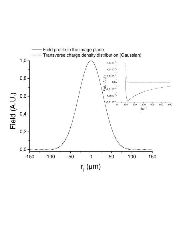
Figure 21: The radial field profile in the image plane (solid line) compared with the Gaussian electron charge density distribution (dotted line). In the inset we show the same plots on a different scale.

4.6 Resolution analysis for incoherent and coherent imaging

No conventional resolution criterion can be applied for the particle spread function in Eq. (80). However, with the help of our method we improved the particle spread function to obtain the ultimate resolution, so that the amplitude particle spread function is now equal to the amplitude point spread function, Eq. (91).

Instead of dealing with the amplitude particle spread functions in Eq. (83) and Eq. (84), we deal with the solution of a simple diffraction problem, where the field produced by a point source is diffracted by a circular pupil. Therefore, the resolution analysis is reduced now to the theoretical framework of standard incoherent or coherent imaging theory (see e.g. BOO1 ). One can take advantage of well-known resolution criteria like the Rayleigh or Sparrow criteria, or alternatively, of a formulation of the resolution problem in terms of Optical Transfer Function (OTF), incoherent case or Coherent Transfer Function (CTF), coherent case.

In principle, our technique could be applied both for incoherent and coherent radiation. However, in the incoherent case, while spatial resolution improves towards the point source, limitations arise due to the small number of photons available. As a result, the method described above is better applied for the coherent imaging case.

When we deal with coherent OTR imaging, limitations of techniques to improve the particle spread function due to a small number of photons can be avoided, given the much larger available photon flux.

As seen before, processing the spatial spectrum and polarization in the Fourier plane allows us to reduce a vectorial problem to a scalar one, so that, instead of dealing with the amplitude particle spread functions in Eq. (83) and Eq. (84) we consider the scalar diffraction pattern in Eq. (91). Thus, the imaging problem is reduced to an imaging problem for coherently radiating point sources.

We note with BOO1 that the Rayleigh criterion is not suitable for defining the resolution in the case of coherent imaging, because it tends to underestimate the minimal distance where resolving two point sources is still possible. An acceptable resolution criterion turns out to be, instead, the Sparrow criterion, stating that the minimal separation of two points on the OTR screen is given by $d\simeq 4.6\cdot\lambdabar/\theta_{a}$. This value may be compared with that given by the Sparrow criterion for incoherent radiation, i.e. $d\simeq 3.0\cdot\lambdabar/\theta_{a}$. Such comparison suggests that incoherent imaging techniques would yield (in the case of point emitters) an ultimate resolution about $1.5$ better than that in the coherent case. However, as explained before, techniques to improve the particle spread function in the incoherent case are limited by the number of photons available.

Finally, it should be clear that the definition of resolution is somewhat arbitrary, as it consists in a single number, a figure of merit to be extracted according to some criterion or algorithm from the actual image. A more quantitative approach to the resolution problem would be to use the CTF representation, where the point spread function is given in terms of its spatial Fourier transform.

Since one has

$$|~{}\mathrm{CTF}~{}|\left({u}\right)\propto\left|\int d\vec{r}_{i}~{}A(\omega,r_{i})\exp[i\vec{u}\cdot\vec{r}_{i}]\right|\propto\mathrm{circ}\left(\frac{uc}{\omega\theta_{a}}\right)~{},$$ (92)

one recovers the result that the pupil behaves like a spatial filter. Spatial frequencies up to $\theta_{a}/\lambdabar$ are allowed to pass through the aperture without distortion, while higher frequencies are blocked. The resolution of the image of the electron bunch reduces to the standard diffraction-limited resolution of a point source.

Let us consider, as a numerical example, our particular case of an XFEL with an ORS setup. Here we are dealing with coherent imaging. As shown above, an acceptable resolution criterion for the coherent imaging case is the Sparrow criterion, which defines the resolution as $d\simeq 4.6\cdot\lambdabar/\theta_{a}$. According to the Sparrow criterion, for our case, i.e. for $\lambda=800$ nm and $\theta_{a}=0.1$, we obtain $d\simeq 6~{}\mu$m.

It should be noted that both Sparrow and Rayleigh criteria can only be applied in the case of a Fraunhofer diffraction pattern from a lens aperture. They cannot be directly applied when one deals with a complicated OTR particle spread function like that in Eq. (82). Therefore, up to now, the diffraction-limited resolution for OTR imaging has been based on the estimation of an ”effective width” of the OTR particle spread function.

For example, in order to estimate the diffraction-limited resolution for the incoherent OTR imager, authors of BENG fit the particle spread function, Eq. (82), to a Gaussian function and calculate the $rms$ width of the Gaussian fit. They conclude that, for $\lambda=800$ nm and $\theta_{a}=0.1$, the particle-spread function given by Eq. (82) has a width of about $6~{}\mu$m, and they consider this as a measure of the diffraction-limited resolution for their system. However, using their method, one concludes that the resolution for a point source is about three times better than what is predicted by the Rayleigh criterion, which is given by $d\simeq 3.8\cdot\lambdabar/\theta_{a}$. In fact, a resolution $d\simeq 1.2\cdot\lambdabar/\theta_{a}$ was reported in BENG for the incoherent case and for a point-source. For example, following BENG , one would obtain a resolution $d\simeq 2~{}\mu$m , while according to the Rayleigh criterion the resolution is $d\simeq 5~{}\mu$m. The difference is due to the use of the width of the point spread function to define the resolution of the system in BENG .

The main result reached in this Section is an optimization of the particle spread function of the system, so that the imaging problem can be reduced to the usual (coherent or incoherent) imaging theory for point-like radiators. This result is summarized in Eq. (91), presenting the amplitude particle spread function of the system after processing, which is equivalent to the amplitude point spread function.

4.7 Comparison of OTR and undulator sources for electron bunch imaging

We have seen that OTR pulses are intrinsically difficult to deal with, due to the presence of the polarization singularity of the OTR field from a single electron, resulting in the space-variant polarization and in the singular behavior of the field amplitude. These difficulties can be avoided for instance if one uses coherent radiation emitted by a modulated electron bunch in the radiator-undulator of the ORS, where the polarization is space-invariant, and the field amplitude has no singular behavior. Yet, coherent undulator radiation is not suitable for imaging applications, while coherent OTR is. In fact, coherent undulator radiation is highly collimated within an angle $\sqrt{\lambdabar/L_{w}}$, $L_{w}$ being the undulator length, which in our case is smaller than a milliradian. Therefore, effectively, the numerical aperture of the imaging system is limited by the divergence of the undulator radiation, defining the resolution of the system. As a result, an electron bunch of a tens-micron-size cannot be resolved with the help of undulator radiation. In contrast to this, the OTR radiation pulse from a single electron has a non-limited angular distribution, and the resolution will only be limited by the numerical aperture of the optical system. This basic characteristics of OTR plays an important role in both coherent and incoherent imaging.

5 Coherent OTR imaging for characterizing electron bunches for XFELs

In the previous Section we have shown that, due to the particular features of the OTR source, the OTR image of a single electron significantly deviates from the image of a point source. This fact causes problems concerning the measure of the charge density distribution. We demonstrated that the resolution can be improved with the help of a polarization transformer and a specific transparency in the Fourier plane at the cost of reduction in photon density. Techniques described in the previous Section can improve the OTR image from a single electron up to the standard diffraction pattern from a point source. We shall now discuss some practical aspects which are specifically related to the characterization of electron bunches in an XFEL system, such as 3D electron bunch structure, signal-to-noise ratio, aberrations and alignment of mask and polarization transformer.

5.1 Electron bunches with spatio-temporal coupling

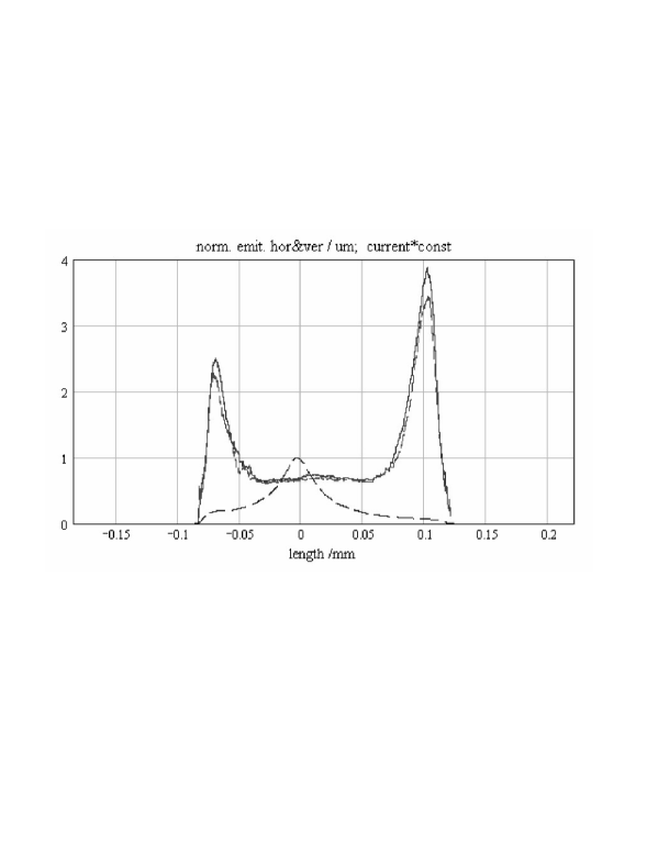
Figure 22: Normalized horizontal and vertical emittance as a function of the longitudinal position within the electron bunch taken from XFEL . The dashed line indicates the peak-current profile.

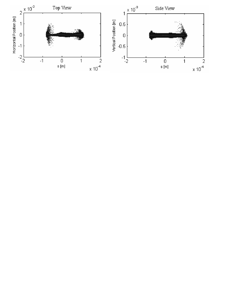
Figure 23: Vertical (left) and horizontal (right) projections of the electron bunch density distribution, BEAM .

The intensity profile in the image plane is readily calculated. In our case of interest radiation is coherent. Therefore, we must convolve, in the space-frequency domain, the field given in Eq. (90) with the Fourier transform of the electron density distribution $\bar{\rho}(\omega,\vec{r})$, and take the squared modulus to get the energy radiated per unit spectral interval per unit surface

$$\frac{d^{2}W}{d\omega dS}(\omega,\vec{r}_{i})=\frac{e^{2}N_{e}^{2}}{\pi^{2}c}\left|\int\d\vec{r^{\prime}}\bar{\rho}(\omega,\vec{r^{\prime}}-\vec{r}_{i})\frac{1}{r^{\prime}}J_{1}\left(\frac{\omega r^{\prime}a}{cf}\right)\right|^{2}~{}.$$ (93)

When dealing with XFEL applications, it is important to realize that the electron-bunch slice emittance changes along the bunch, as one can see from the example shown in Fig. 22, which refers to the European XFEL XFEL . Note that even if the slice emittance were constant, some mismatch is always present, leading to a dependence of the electron bunch transverse size on the longitudinal coordinate (see Fig. 23). A comparison of Fig. 22 with Fig. 23 shows that even in the part of the electron bunch where the emittance does not vary much there are significant changes in the transverse size. As a matter of fact, XFEL beam formation systems will generate electron bunches that exhibit a coupling between space and time even in the case of nominal operation. As a result, optical replica pulses will also exhibit coupling between space and time, i.e. the electric field components in the space-frequency domain cannot be factorized as a product $\widetilde{E}(\omega,\vec{r})=f(\vec{r})g(\omega)$.

Figure 24: Effect of the bandpass optical filter on recording the bandwidth-limited optical replica pulse by a single detector pixel.

Figure 25: Schematic diagram of coherent OTR imaging of electron bunch without bandpass optical filter.

Figure 26: Schematic diagram of coherent OTR imaging of electron bunch with bandpass optical filter. The setup with bandpass optical filtering can be used to reconstruct the (x,y) electron bunch projection.

Figure 27: Setup of high-resolution coherent OTR imager with bandpass optical filter to reconstruct the (x,y) electron bunch projection.

The detector automatically performs an integration over time of the intensity $I(t,\vec{r}_{i})$ in the space-time domain, which can be extended over all times, because the detector is not fast enough to resolve a single radiation pulse. Such integration over times is equivalent, due to Parseval’s theorem, to an integration over all frequencies of Eq. (93). Therefore, the detector will record the energy per unit surface

$$\frac{dW_{\mathrm{det}}}{dS}(\vec{r}_{i})\propto\int_{-\infty}^{\infty}d\omega\left|\int\d\vec{r^{\prime}}\bar{\rho}(\omega,\vec{r^{\prime}}-\vec{r}_{i})A(\omega,r^{\prime})\right|^{2}~{}.$$ (94)

Let us define ${\rho}_{0}(t,\vec{r})$, as the electron density distribution of the unmodulated electron bunch. In the case of a bunch modulated with frequency $\omega_{m}$, ${\rho}_{0}(t,\vec{r})$ and ${\rho}(t,\vec{r})$ are linked by

$${\rho}(t,\vec{r})={\rho}_{0}(t,\vec{r})[1+a_{f}\cos(\omega_{m}t)]~{},$$ (95)

where $a_{f}$ is the modulation level. Let us also call $\bar{\rho}_{0}(\omega,\vec{r})$ the Fourier transform of $\rho_{0}(t,\vec{r})$ with respect to time.

Since the adiabatic approximation applies, the function $\bar{\rho}(\omega,\vec{r})$ has a narrow bandwidth $\Delta\omega/\omega\ll 1$. Thus, we can write $\bar{\rho}(\omega,\vec{r})=\bar{\rho}_{0}(\omega-\omega_{m},\vec{r})a_{f}$, $a_{f}$ being the modulation amplitude. Note that here we assume $a_{f}=\mathrm{const}$, an assumption justified in Section 2, where we discussed that the main goal of the ORS setup is to produce an exact optical replica of the electron bunch. Since $\rho_{0}(t,\vec{r})$ is a positive function and $a_{f}$ is constant, the optical pulse is automatically bandwidth limited.

The situation is described in the time domain by Fig. 24 (top) and Fig. 25. The fact that $\bar{\rho}(\omega,\vec{r})=\bar{\rho}_{0}(\Delta\omega,\vec{r})a_{f}~{}$, where $\Delta\omega=\omega-\omega_{m}$, is implied by the validity of Eq. (95) with $a_{f}=\mathrm{const}$. Note that if $a_{f}$ were not constant, $\bar{\rho}(\omega,\vec{r})$ would be a convolution of $\bar{\rho}_{0}(\Delta\omega,\vec{r})$ with the Fourier transform of $a_{f}$.

In Fig. 24, the envelope of the optical replica pulse seen by a single pixel of the detector is shown as a function of time. This function is integrated by the detector pixel over a given temporal interval, which is longer than the duration of the pulse. As shown in Fig. 24, the result is proportional to the time-integrated squared modulus of the amplitude of the pulse envelope. In its turn, the pulse envelope can be written as a convolution between $\rho_{0}(t,\vec{r})$ and the point spread function $A(\omega_{m},r)$, where the point spread function is calculated at $\omega=\omega_{m}$ because the adiabatic approximation holds. The detector thus records

$$\frac{dW_{\mathrm{det}}}{dS}(\vec{r}_{i})\propto\int dt\left|\int dr^{\prime}\rho_{0}(t,\vec{r^{\prime}}-\vec{r}_{i})A(\omega_{m},r^{\prime})\right|^{2}~{},$$ (96)

which is equivalent to Eq. (94) by means of Parseval’s theorem. Neglecting the blurring one simply obtains

$$\frac{dW_{\mathrm{det}}}{dS}(\vec{r}_{i})\propto\left\langle\rho_{0}^{2}\right\rangle=\int dt\left|\rho_{0}(t,-r_{i})\right|^{2}~{}.$$ (97)

The right hand side of Eq. (97) is an integral in time of the squared modulus of the charge density distribution, i.e. it is a quadratic projection, along the temporal axis, of the charge density distribution.

Note that in the case of incoherent OTR imaging (still neglecting the blurring) one would sum the intensity of all electrons independently. As a result, in order to obtain the energy absorbed by a detector pixel at a given transverse position $\vec{r}_{i}$, we need to sum over all the electron arrival times. Therefore, the signal from each pixel will be proportional to the integral in time of $\rho_{0}(t,\vec{r}_{i})$, i.e. it is a linear projection of $\rho_{0}(t,\vec{r}_{i})$ along the temporal axis.

Both linear and quadratic projections can be taken advantage of. They can be used for comparison with results of numerical simulations and they are both sensitive to perturbations of the transverse size of the bunch, which we need to monitor.

However, also in the coherent OTR imaging case it is possible to obtain the linear projection of the charge density distribution, instead of the quadratic projection, by inserting a narrow-band optical filter with bandwidth much smaller than the inverse duration of the optical pulse, and centered at the modulation frequency $\omega_{m}$. Calling with $\mathcal{G}(\omega-\omega_{m})$ the filter transfer function, one obtains the following modification to Eq. (94)

$$\frac{dW_{\mathrm{det}}}{dS}(\vec{r}_{i})\propto\int_{-\infty}^{\infty}d\omega\left|\int\d\vec{r^{\prime}}\bar{\rho}(\omega,\vec{r^{\prime}}-\vec{r}_{i})\mathcal{G}(\omega-\omega_{m})A(\omega,r^{\prime})\right|^{2}~{}.$$ (98)

(99)

Due to the narrow-band nature of $\mathcal{G}$, and remembering that due to the adiabatic approximation $\bar{\rho}(\omega,\vec{r})=\bar{\rho}_{0}(\omega-\omega_{m},\vec{r})a_{f}$, both $\bar{\rho}$ and $J_{1}$ can be taken out of the integral in $d\omega$, thus yielding

$$\frac{dW_{\mathrm{det}}}{dS}(\vec{r}_{i}) \propto a_{f}^{2}\int_{-\infty}^{\infty}d\omega\left|\mathcal{G}(\omega-\omega_{m})\right|^{2}\cdot\left|\int\d\vec{r^{\prime}}\bar{\rho}_{0}(0,\vec{r^{\prime}}-\vec{r}_{i})A(\omega_{m},r^{\prime})\right|^{2}~{}.$$ (100)

In the time domain, the envelope of the optical replica pulse (see also Fig. 24) coincides with the non-modulated electron density distribution, $\rho_{0}(t,\vec{r})$. One has

$$\bar{\rho}_{0}(0,\vec{r}_{i})=\int_{-\infty}^{\infty}dt\rho_{0}(t,\vec{r}_{i})~{}.$$ (102)

Note that $\bar{\rho}_{0}(0,\vec{r}_{i})$ is a positive function, in contrast with the complex-valued function $\bar{\rho}_{0}(\Delta\omega,\vec{r}_{i})$ for $\Delta\omega\neq 0$. One sees that the detector just records the squared modulus of linear projection (in time) of the charge density distribution.

The same conclusion can be reached directly in the time domain by inspecting Fig. 24 (bottom) and Fig. 26. The optical-replica pulse is stretched by the optical filter to a duration of $1/(\Delta\omega)\gg\tau_{p}$, with $\tau_{p}$ the duration of the original optical replica pulse. The result of this operation is another pulse whose envelope is given by the convolution between the envelope $\rho_{0}(t)$ and the Fourier Transform of $\mathcal{G}$. Since $1/(\Delta\omega)\gg\tau_{p}$, the detector pixel sees the integrated intensity, that is just given by Eq. (102). A possible setup for high-resolution OTR imaging for XFEL setups including a bandpass filter is shown in Fig. 27.

In closing, it is interesting to note that in the incoherent case one sums up intensities from single particle contributions. For example, in the case of the usual incoherent OTR setup in Fig. 10 (with no image processing), the energy per unit surface in the image plane is given by:

$$\frac{dW^{\mathrm{incoh}}_{\mathrm{det}}}{dS}(\vec{r}_{i})\propto\int_{-\infty}^{\infty}d\omega\int\d\vec{r^{\prime}}\bar{\rho}(0,\vec{r^{\prime}}-\vec{r}_{i})\left|A_{p}(\omega,r^{\prime})\right|^{2}~{},$$ (103)

which already presents a linear projection of the charge density distribution. From Eq. (103) we see that, in the incoherent case, the spectral energy density per unit surface is proportional to $\bar{\rho}(0,\vec{r}_{i})$ (neglecting the blurring), i.e. to the Fourier transform of the charge density distribution at zero frequency. This follows from an average over ensembles. In Eq. (103), $\bar{\rho}(0,\vec{r}_{i})$ may also be presented as $\bar{\rho}(0,\vec{r}_{i})=\int\rho(t,\vec{r})dt$. Then, based on Eq. (95), which is valid in general, due to adiabatic approximation we have $\int\rho(t,\vec{r})dt=\int\rho_{0}(t,\vec{r})dt$, for arbitrary modulation strength $a_{f}(t,\vec{r})$.

5.2 Effect of aberrations on the performance of coherent optical systems

When an optical system acts as a linear, space-invariant filter for a complex field amplitude, it is referred to as isoplanatic. When a coherent optical system is isoplanatic, the effect of aberrations on its performance can be treated within the framework of a standard theory MILL . However, in general, even aberration-free optical systems are not isoplanatic. Some spatial phase distortion is unavoidably introduced, which severely modifies the intensity distribution of the image.

In section 4 we discussed the effect of non-isoplanatism on coherent image formation. We demonstrated that thin aberration-free lenses can only be considered as isoplanatic system if limitations (57) are satisfied. Here we discuss the effect of non-isoplanatism on coherent imaging of extended objects when the thin lenses composing the optical system are no more aberration-free, and we discuss conditions when the standard isoplanatic theory can be applied.

Figure 28: Isoplanatic system in case of aberrations. When wavefront errors exist, we can imagine that a phase-shifting plate is placed at the aperture, thus deforming the wavefront. When the characteristic scale of the wavefront errors $a^{\prime}$ is much larger than a single Fresnel zone, and the object scale $\sigma$ is much smaller than $a^{\prime}$, the optical system with aberrations is isoplanatic. The amplitude transfer function concept can be applied to such system and the generalized pupil function plays the role of the amplitude transfer function. In this case, left and right configurations are equivalent.

Consider Fig. 28. Aberrations, i.e. wavefront errors, can be imagined as equivalent to a phase-shifting plate located at the aperture, which deforms the wavefront. The complex amplitude transmittance $T(\vec{r}^{\prime})$ of the phase-shifting plate is given by

$$T(\vec{r}^{\prime})=\exp[i\Phi(\vec{r}^{\prime})]~{},$$ (104)

where $\Phi(\vec{r}^{\prime})$ characterizes the aberration. As before, we indicate with $P(r^{\prime})$ the pupil function characterizing the lens aperture. The complex function $P(r^{\prime})T(\vec{r}^{\prime})$ is referred to as the generalized pupil function.

When an aberrated optical system is isoplanatic, the amplitude point spread function of the system is space-invariant, and is simply given by the Fraunhofer diffraction pattern of the generalized pupil function $P(r^{\prime})T(\vec{r}^{\prime})$, which is essentially its Fourier transform. The generalized pupil function itself plays the role of the amplitude transfer function for the system. In this case, the spatial bandwidth of the amplitude transfer function is limited by the finite pupil aperture $P(r^{\prime})$. The effect of aberrations consists in the introduction of phase distortions within the bandwidth of the amplitude transfer function. These phase distortions can have a severe effect on the fidelity of the imaging system.

Conditions for an aberrated optical system to be isoplanatic are easily derived on the basis of Section 4.2. Let us call with $a^{\prime}$ the characteristic scale of the wavefront error. Suppose now that $a^{\prime}$ is much larger than a single Fresnel zone, and that the object scale $\sigma$ is much smaller than $a^{\prime}$. In this case, the reasoning in Section 4.2 can be repeated replacing conditions (57) with

$$\sigma\ll a^{\prime}~{},~{}~{}~{}~{}a^{\prime 2}/(\lambdabar f)\gg 1~{}.$$ (105)

Then, both Eq. (55) and Eq. (62) can be recovered, and the optical system is isoplanatic.

More generally, geometrical aberrations are described by the Siedel wavefront representation BORN :

$$\Phi(r^{\prime},\theta)=b_{20}\left(\frac{r^{\prime}}{a}\right)^{2}+b_{40}\left(\frac{r^{\prime}}{a}\right)^{4}+b_{31}\left(\frac{r^{\prime}}{a}\right)^{3}\cos(\theta)+b_{22}\left(\frac{r^{\prime}}{a}\right)^{2}\cos^{2}(\theta)~{},$$ (106)

where $b_{20}$, $b_{40}$, $b_{31}$ and $b_{22}$ are the amounts of defocus, spherical aberration, coma, and astigmatism. The quantities $r^{\prime}$ and $\theta$ are defined through

$$r^{\prime 2}\equiv(x^{\prime})^{2}+(y^{\prime})^{2}~{},~{}~{}~{}~{}~{}\theta\equiv\tan^{-1}(x^{\prime}/y^{\prime})~{}.$$ (107)

For the sake of illustration, it is interesting to discuss a particular example for the case of defocusing aberrations. In this case it is customary to introduce a quadratic phase error $\Phi(r^{\prime})$ in the form

$$\Phi(r^{\prime})=b_{20}\left(\frac{r^{\prime}}{a}\right)^{2}~{},$$ (108)

In Eq. (108), the characteristic scale $a^{\prime}$ is linked to the aberration strength by $a^{\prime 2}\sim a^{2}/b_{20}$. Therefore, from the second condition in (105), one has $b_{20}\ll a^{2}/(\lambdabar f)$, which means that $b_{20}$ should be much smaller than the number of Fresnel zones on the aperture. Similarly, from the first condition in (105) one has $b_{20}\ll a^{2}/\sigma^{2}$, meaning that the aberration strength should be much smaller than the ratio between the aperture area and the object area too. Note that these conditions actually set criteria for the system to be isoplanatic in terms of aberration strength, diffraction, and geometrical dimension of the source compared with the pupil aperture $a$. Finally, note that in general, for an aberration of order $n$, the aberration strength should satisfy the conditions $b_{nm}^{2/n}\ll a^{2}/(\lambdabar f)$ and $b_{nm}^{2/n}\ll a^{2}/\sigma^{2}$.

In our case of coherent OTR imaging, the impact of chromatic aberrations on the system resolution can be avoided by taking advantage of the narrow bandwidth of the optical replica radiation pulse.

5.3 Sensitivity to displacement of mask and polarization transformer away from the focal plane

Up to now we discussed two cases: a pupil consisting of a finite aperture only, and a pupil consisting of a finite aperture with aberrations.

In the case of a pupil without aberrations we saw, Fig. 13, that conditions (57) guarantee that the system is isoplanatic. The field in the Fourier plane is the product of the Fourier transform of the field at the object plane and the pupil function (see Eq. (58)). Based on Eq. (58), we demonstrated that the position of the aperture can be located anywhere between lens and focal plane.

Figure 29: Introduction of a mask in the pupil. The problem is related to the so called inverse apodization. In this case the generalized pupil function $P(r)T_{m}(r)$ has no characteristic size and, generally speaking, the optical system is non-isoplanatic. For coherent imaging of extended object some spatial phase distortions is introduced, which severely modifies the low (spatial) frequency components of the object spectrum.

This reasoning was extended to the case of aberrations in the previous Section 5.2. There we saw, Fig. 28, that the same conclusions can be drawn whenever conditions (105) hold, which have the same mathematical structure of conditions (57), with the only difference that they now include the characteristic scale of the wavefront error $a^{\prime}$ and not the size of the pupil aperture $a$.

Both the problems that we discussed are related to coherent image formation theory. This knowledge can be applied to treat related technical issues.

The goal of this subsection is to deal with the problem of alignment of optical elements along the optical axis. As was shown in Section 4.1, Fig. 13, a lowpass spatial frequency filter under conditions (57) is insensitive to the position of the filter (which can be located anywhere between lens and focal plane positions).

It is now a good time to generalize our considerations, and to examine the sensitivity to displacement of a Fourier mask of particular interest. The mask that we want to consider has a profile given in Eq. (87), Fig. 29. This profile changes the shape of the optical transmission of the optical system. Such changing is known in literature as apodization. Our case is actually known as inverse apodization (see e.g. GOOD ) because it suppresses the central part, and not the periphery of the optical signal.

Considerations made above will lead us to find isoplanatic conditions for a pupil with inverse apodization. The pupil function in this case given by the product $P(r)T_{m}(r)$.

We start with Eq. (55) assuming that the second of conditions (57) is satisfied. This time, we analyze Eq. (55) in a different way. Expressing ${F}(0,\vec{u})$ in terms of a Fourier integral, neglecting the quadratic phase factor in $u^{2}$ because of the second of conditions (57), and integrating in $d\vec{u}$ we obtain

$${\widetilde{E}}\left(2f,\vec{r}_{f}\right)=\frac{i\omega}{2\pi cf}\int d\vec{r^{\prime}}~{}\widetilde{E}\left(0,\vec{r^{\prime}}\right)P(\vec{r}_{f}-\vec{r^{\prime}})T_{m}(\vec{r}_{f}-\vec{r^{\prime}})\exp\left[-\frac{i\omega\vec{r^{\prime}}\cdot\vec{r}_{f}}{cf}\right]~{}.$$ (109)

(110)

Now $\widetilde{E}\left(0,\vec{r^{\prime}}\right)$ is our object, whose extension we estimate with the characteristic size $\sigma$.

We begin by analyzing the case without mask, i.e. $T_{m}(r)=1$, using Eq. (110). If also the first of conditions (57) is verified, $\sigma\ll a$, then we can have $\sigma^{2}/(\lambdabar f)\sim 1$, meaning that the pupil is in the near zone. Since $r^{\prime}\lesssim\sigma$ (otherwise the field at $z=0$ under the integral vanishes), due to the exponential factor in Eq. (110), one is actually limited to the range $r_{f}\lesssim\sigma$. Then, $P(\vec{r_{f}}-\vec{r^{\prime}})=1$, because $|\vec{r_{f}}-\vec{r^{\prime}}|\lesssim\sigma\ll a$. Therefore, the pupil function $P$ can be taken out of the integral sign in Eq. (110), meaning that it does not perturb the image of the object. In the case $\sigma^{2}/(\lambdabar f)\ll 1$, since $r^{\prime}\lesssim\sigma$, the exponential term in Eq. (110) is of order unity for maximal values of $r_{f}\sim\lambdabar f/\sigma\gg\sigma$. Now the pupil operates as a cutoff filter, introducing a little blurring of the sharp edge on a scale $\sigma\ll a$.

Now let us turn back to the case a mask with inverse apodization is present. We can appreciate the difference compared to the previous case. When $\sigma^{2}/(\lambdabar f)\sim 1$ we cannot take the generalized pupil function $P(r)T_{m}(r)$ out of the integral sign anymore, because on the scale $r_{f}\sim\sigma$ (determined by imposing that the exponential term in Eq. (110) be at most of order unity) we have significant variation of the generalized pupil function through $T_{m}(r)$, which does not present any characteristic scale of interest. When instead $\sigma^{2}/(\lambdabar f)\ll 1$, we have the characteristic scale $r_{f}\sim\lambdabar f/\sigma\gg\sigma$. Then, with accuracy $\sigma^{2}/(\lambdabar f)$ we can take the generalized pupil out of the integral sign, because for these large values of $r_{f}$ the result of the integration changes little within excursions of $r^{\prime}\lesssim\sigma$.

A qualitatively different result is reached, because low frequencies are always perturbed, while in the case of a simple pupil $P(\sigma)=1$ for $\sigma\ll a$. It is therefore impossible to apply the concept of amplitude transfer function to the system in Fig. 29. In other words, the system is not isoplanatic.

Note that inverse apodization is discussed in literature only in relation with incoherent imaging. If we were imaging an incoherent collection of point sources the problem of isoplanatism would not exist at all, and the autocorrelation function of the pupil actually would serve as transfer function of the system. However, this observation applies to an object consisting of an incoherent collection of point sources only, and not to the case of incoherent OTR imaging, where we deal with an incoherent collection of laser-like sources. In this case, each source has a finite transverse extent, and the problem of isoplanatism exists exactly as in the coherent case.

Figure 30: In our case of interest, the largest transverse electron-bunch size is small enough for its Fraunhofer diffraction pattern to be formed at the pupil plane. As a result, the most important part of the object spectrum (mid-range and high spatial frequencies) meet isoplanatic condition. For this range the generalized pupil function plays the role of amplitude transfer function. Perturbations of low frequency components of the object spatial spectrum can only modify the intensity distribution on a scale of much larger size compared to the bunch size.

Figure 31: When the transverse size of the electron bunch is small enough for its Fraunhofer diffraction pattern to be formed at the pupil plane, mask and polarization transformer can be installed at arbitrary position within the focal distance.

Clearly, as soon as we consider inverse apodization for coherent imaging, the situation becomes complicated. Nevertheless the isoplanatic conditions (105) can be satisfied for mid-range and high spatial frequencies of the object spectrum. Fortunately, in the XFEL case perturbations of the low spatial frequency components lead to the introduction of some background only, but not distortions in the electron-bunch image (see Fig. 21).

Considering the specifics of our problems as illustrated in Fig. 30, we are interested in spatial frequencies higher than $1/\sigma$, where $\sigma$ is the largest size of interest in our object. Thus, we are not interested in spatial frequencies lower than $1/\sigma$, which are modified by a shift in the mask position. This reasoning yields an effective scale $a^{\prime}$ on the inverse apodized pupil of order $a^{\prime}\sim\lambdabar f/\sigma$. Such scale can be used in conditions (105), which are now equivalent to

$$\frac{\sigma^{2}}{\lambdabar f}\ll 1~{}.$$ (111)

When condition (111) is satisfied, i.e. when the lens is in the far zone with respect to the object structure of size $\sigma$, conditions (105) are satisfied too, and one can shift the mask from the focal plane without appreciable effects.

The far-zone condition (111) means that the transverse size of the object is much smaller than the size of the Fourier pattern. Intuitively, as it can be seen from Fig. 31, when placed in the far-zone, the lens transforms a spherical wavefront from a point source into a plane wave. When the object has some transverse dimension $\sigma$, such that $\sigma^{2}/\lambdabar f\ll 1$, one can neglect Fresnel diffraction effects at the mask placed anywhere between pupil and Fourier plane. Thus, with accuracy $\sigma^{2}/\lambdabar f$, the wavefront behind the lens can be still considered plane and does not change at any position between lens and focal plane.

As a result, in the far zone, there is a very low sensitivity to mask and polarization-transformer displacement from the focal plane.

5.4 Sensitivity to transverse displacement for mask and Polarization Transformer

With the help of a polarization transformer and a Fourier-plane mask, as schematically illustrated in Fig. 18, we have seen in the previous Section that spatial spectrum and polarization of OTR radiation can be conveniently processed.

A schematic representation of the polarization transformer is shown in Fig. 32. The polarization transformer demonstrated in POLA , POL2 is composed of eight POLA up to twelve POL2 sectors of half-wave retardation plates, each one with different orientation of the crystal’s ”fast” axis. The linear dimension of the device is of the order of a centimeter. A photonic crystal segmented half-wave-plate is the perfect radial-to-linear polarization converter for coherent OTR imager. For a twelve segments device, the linear polarization purity can be as high as $99\%$, with transformation efficiency of about $92\%$. Due to the good quality of the photonic crystal segmented half-wave-plates, the incident wavefront is negligibly perturbed.

Figure 32: Segmented half-wave plate with octonary sectors. Arrows schematically show the direction of the fast axis of the crystal in each sector.

Both mask and polarization transformer are endowed with rotational invariance. Their centers of rotation should coincide with the position of the optical axis, where the center of the Fourier transform is located. The accuracy needed in the alignment of the Fourier-plane mask and the polarization transformer is related to the fact that we wish to obtain a proper image within region B in Fig. 7, i.e. $r_{i}\lesssim 100~{}\mu$m in the image plane for a focal distance $f\simeq 30$ cm. This maximal value of $r_{i}$ corresponds to a region in the focal plane given by $r_{f}\gtrsim\lambdabar f/r_{i}\simeq 400~{}\mu$m. Within this accuracy, the electron bunch image will not be sensitive to transverse displacements of the center of the mask in the Fourier-plane and of the polarization transformer with respect to the optical axis. This estimation also specifies the required manufacturing accuracy, close to the center of rotation, of the polarization transformer and of the mask in the Fourier-plane, which should be in the range of about $100~{}\mu$m.

5.5 Signal-to-noise Ratio

The signal-to-noise ratio of our system is strictly related to the practical resolution achievable. In fact, one has to make sure that the number of photons available are enough to allow implementation of the imaging scheme described above.

As an example, let us consider the case when the detector is a CCD camera. Supposing that the CCD charge capacity is about $2\div 4\cdot 10^{4}$ electrons per pixel, and assuming a quantum efficiency of about $50\%$, one concludes that the CCD camera will saturate at about $10^{5}$ photons per pixel or more.

For our particular case of coherent OTR imaging, the estimated resolution according to the Sparrow criterion is about $6~{}\mu$m. Because of the Nyquist sampling theorem, the CCD pixel size should be about $3~{}\mu$m. A typical CCD pixel size is about $10\times 10~{}\mu\mathrm{m}^{2}$. Thus, to resolve $6~{}\mu$m features in the electron bunch, the magnification of the optical system should be about $1:3$ or more. Choosing for simplicity the magnification $1:3$, our zone of interest (region B in Fig. 7) will result in an image size of $300\times 300~{}\mu\mathrm{m}^{2}$ in the image (detector) plane, i.e. $30\times 30$ pixels. Similarly, the electron bunch density distribution (region A in Fig. 7) of order of $30~{}\mu$m is imaged into an area of about $100\times 100~{}\mu\mathrm{m}^{2}$, i.e. $10\times 10$ pixels.

Assuming $10^{12}$ photons in the region of interest of the imaging system (region B in Fig. 7), we obtain about $10^{9}$ photons per pixel. The difference of four orders of magnitude beyond the saturation level of the CCD can be used to implement the particle-spread function improvement described in the previous Section, which may be quite expensive in terms of photon budget.

Obviously, in any case, we should make sure that no pixel on the CCD camera gets more than $10^{5}$ photons. From Poisson statistics follows that the shot-noise level at saturation is about a fraction of a percent of the signal, i.e. the signal-to-noise ratio is a few hundreds. Shot noise is the dominant cause of noise at high photon-level conditions. However, while the signal decreases, other sources of noise become important. As the photon level drops, also the shot noise level diminishes, and the CCD camera tends to become read-out-noise limited. Assuming a read-out noise e.g. of order of $10$ electrons, a certain pixel operates in read-out-noise limited regime when the number of photons incident on that pixel is of order $10^{2}$ or less. At this photon level the shot-noise and the read-out noise are comparable. The signal-to-noise ratio is of order $10$, and quickly decreases as the number of photons decreases. The dynamical range of our device is therefore of about $4$ orders of magnitude, i.e. the ratio between the full-well capacity and the read-out noise.

6 3D electron-bunch imaging from diffraction intensity measurements by use of iterative phase-retrieval methods

Up to now we proposed to process the particle spread function of the OTR imager in order to improve the overall resolution of the system. We proposed to use coherently generated radiation but, from a fundamental viewpoint, techniques described in the previous Section maybe implemented for incoherent radiation as well. The only problem using incoherent radiation is linked with the smaller number of available photons, compared to the coherent case, which makes the discussed technique unpractical. In other words, up to now we took advantage of the coherent nature of OTR in the sense that we exploited the large number of available photons.

The fact that we are dealing with coherent radiation, however, opens up new imaging possibility. Namely, the detector can be directly installed in the Fourier plane, and imaging from diffraction intensity measurements can be enforced. Once the Fourier transform of the object is known, the recovery of the image is reduced to the calculation of an inverse Fourier transform. However, one can only measure the modulus of the Fourier transform, and a phase-retrieval problem arises. With their algorithm GERC , Gerchberg and Saxton demonstrated that numerical solutions to the two-dimensional phase retrieval problem is possible. A number of phase-retrieval algorithms were developed based on the original Gerchberg-Saxton algorithm. For the interested reader we refer to extensive reviews on the subject FINN -LUKE .

Two issues need to be mentioned, which may affect the usefulness of the iterative phase-recovery method for our case. The first is the problem of uniqueness of the reconstructed object, the second is the speed of the algorithm, which may not be fast enough to perform coherent OTR imaging at an acceptable repetition rate.

In the following we will study two cases when object and propagated field are related by a Fourier transform. In the first case, the detector is placed in the focal plane of a lens. In the second, it is placed in the far (Fraunhofer) zone of the propagated field. The lens setup allows one to control the image parameters, but it can potentially introduce aberrations. The lensless setup instead, is defined by the position of the detector only.

6.1 Lens-based setup for diffractive imaging

6.1.1 Deconvolution by Fourier-plane mask

Figure 33: Lens-based setup for diffractive imaging of an electron bunch.

Let us consider the setup in Fig. 33. A lens is used to obtain the Fourier transform of the object in the focal plane. Once the squared modulus of the Fourier transform of the object is recorded, the object can be reconstructed with the help of an iterative phase-retrieval algorithm.

Let the object be placed in the front focal plane of the lens. The field across the back focal plane is given by Eq. (58), where we neglect lens imperfections, and assume that conditions (57) are satisfied. By means of the convolution theorem, the (spatial) Fourier transform of the field in the object plane, which enters Eq. (58), is given by the product of the Fourier transform of the single-particle field and the Fourier transform of the charge density distribution, $\varrho(\omega,\vec{u})$. Note that here we are discussing a 3D Fourier transform, both with respect to time and space. In other words, $\varrho(\omega,\vec{u})$ is the 3D Fourier transform of $\rho(t,\vec{r})$:

$$\varrho(\omega,\vec{u}~{})=\int d\vec{r}dt~{}\rho(t,\vec{r})\exp[i\vec{r}\cdot\vec{u}~{}]\exp[i\omega t]~{}.$$ (112)

Accounting for the vectorial nature of the OTR field, Eq. (58) can be written as

$$\vec{\widetilde{E}}\left(2f,\vec{r}_{f}\right)=\frac{2N_{e}e\gamma^{2}\vec{r}_{f}}{c(\gamma^{2}r_{f}^{2}+f^{2})}\varrho\left(\omega,-\frac{\omega\vec{r}_{f}}{cf}\right)P(\vec{r}_{f})~{}.$$ (113)

Figure 34: Reconstruction of an object from the modulus of its Fourier transform by using an iterative phase-retrieval method. For the electron-beam imager problem the a-priory constraint is the object nonnegativity. For this support phase retrieval is much easier and almost always unique. The method will open up the possibility of real-time, wavelength-limited optical imaging of electron bunches.

Figure 35: Structure of the coherent OTR radiation pattern as observed in the Fourier plane. Parameters are as in Fig. 7.

The intensity in the Fourier plane is thus given by

$$I(\omega,\vec{r}_{f}) = \frac{d^{2}W}{d\omega dS}=\frac{c}{4\pi^{2}}\left|\vec{\widetilde{E}}\left(2f,\vec{r}_{f}\right)\right|^{2}$$ (114)

$$= \frac{N_{e}^{2}e^{2}\gamma^{4}r_{f}^{2}}{\pi^{2}c(\gamma^{2}r_{f}^{2}+f^{2})^{2}}\left|\varrho\left(\omega,-\frac{\omega\vec{r}_{f}}{cf}\right)\right|^{2}\left|P(\vec{r}_{f})\right|^{2}~{}.$$ (115)

The processing of the intensity is better explained in Fig. 34, where the part of the scheme after the lens is zoomed-in. The detector is installed in the Fourier plane.

The structure of the coherent OTR radiation pattern as observed in the Fourier plane is shown in Fig. 35. We are interested in the intensity distribution in the Fourier plane, in contrast to the previously discussed cases when we were interested in the intensity distribution in the image plane. The situation is much simpler: in fact, Eq. (LABEL:Fplane2mody) consists of the product of a single-particle factor, the squared electron bunch structure factor, and the squared pupil function. This is due to the fact that the polarization of the coherent OTR field in the Fourier plane is radial, with respect to the optical axis, exactly as the polarization of a single-electron OTR field. This property greatly simplifies the image processing, because we do not need a polarization transformer to deconvolve the electron bunch structure factor in the Fourier plane.

Separation of the squared modulus of the spatial Fourier transform of the charge density distribution from the squared modulus of the spatial Fourier transform of the amplitude particle spread function may be done at software level, by taking the ratio of the experimental data with the (known) squared modulus of the spatial Fourier transform of the amplitude particle spread function. An alternative possibility is to insert a filter in the Fourier plane, as shown in Fig. 33. The mask to be inserted has the same characteristics discussed in the previous Section 4.5.2. Note that here we are considering a range of $r_{f}$ such that $r_{f}/f\gg 1/\gamma$. This is our range of interest because the electron beam dimension $\sigma_{r}\ll\gamma\lambdabar$ (see Section 3) is reciprocally related to the high spatial-frequency limit, so that the relativistic factor $\gamma$ cancels out in Eq. (LABEL:Fplane2mody). Therefore, Eq. (LABEL:Fplane2mody) is independent of $\gamma$, and the mask transmittance is given by $T_{m}(r)$ in Eq. (87).

Note that here we implicitly assumed that a bandpass filter is used, as discussed in the previous Section, to generate a linear integral of the signal. Since such filter is tuned at $\omega_{m}$, the intensity in the detector plane behind the mask and the bandpass filter is

$$I(\omega_{m},\vec{r}_{f}) = \mathrm{const}\cdot\left|\varrho\left(\omega_{m},-\frac{\omega_{m}\vec{r}_{f}}{cf}\right)\right|^{2}\left|P(\vec{r}_{f})\right|^{2}$$ (117)

$$= \mathrm{const}\cdot a_{f}^{2}\left|\varrho_{0}\left(0,-\frac{\omega_{m}\vec{r}_{f}}{cf}\right)\right|^{2}\left|P(\vec{r}_{f})\right|^{2}~{},$$ (118)

where (see Eq. 95) $\varrho(\omega_{m},\vec{u})=a_{f}\varrho_{0}(0,\vec{u})=a_{f}\int_{-\infty}^{\infty}dt\Phi(t,\vec{u})$, where $\Phi$ is the spatial Fourier transform of $\rho_{0}(t,\vec{r})$. The main difference to be remarked here, with respect to the discussion in the previous Section, is that for diffractive imaging one needs a bandpass filter, while in the previous Section one could choose between a linear or a quadratic integral projection of the signal. In fact, without a filter, one would record $\int d(\Delta\omega)|\varrho_{0}(\Delta\omega,\vec{u)}|^{2}$, and it would be problematic to reconstruct the structure of the electron bunch in real space. On the contrary, once $|\varrho_{0}(0,{\omega_{m}\vec{r}_{f}}/({cf}))|^{2}$ is measured, the solution of the phase retrieval problem yields back $\bar{\rho}_{0}(0,\vec{r})=\int_{-\infty}^{\infty}dt\rho_{0}(t,\vec{r})$. Note that the filter should have a bandwidth smaller than the bandwidth of $\bar{\rho}_{0}(\Delta\omega,\vec{r})$.

6.1.2 Phase-retrieval problem

Once the squared modulus of the spatial Fourier transform of the electron-bunch projection along the time axis, $|\varrho_{0}(0,\omega_{m}\vec{r}_{f}/({cf}))|^{2}$, is obtained, one deals with a typical phase-retrieval problem. In fact, in order to reconstruct the object one needs to know both amplitude and phase of the diffraction field. However, the only directly-measurable quantity in the Fourier plane is the intensity, which is proportional to the squared modulus of the field. Determination of the missing phase from the observed intensity is known as phase-retrieval. In our case, $\varrho_{0}$ must be obtained from the knowledge of $|\varrho_{0}|^{2}$. Only when the phase of $\varrho_{0}$ is known one can retrieve the object $\bar{\rho}_{0}(0,\vec{r})$.

The phase retrieval is typically based on an Iterative Transform Algorithm (ITA) GERC , FINN -LUKE . This cycles between real and reciprocal space, enforcing known constraints. In the reciprocal space, the known constraint is, naturally, the modulus of the Fourier transform of the object.

In the real space, some generic constraints are usually granted too. First, any physical object is square-integrable. Moreover, in real space, a finite support can be defined for any optical system. The support is defined as the set of points over which the object is nonzero, a finite support meaning that the object is nonzero only within a finite region of space. The shape of the object is usually required to be known in order to set the support constraint in the ITA. This support is typically larger than the actual boundary of the object, in which case it is said to be loose. A method for finding an estimate of the loose support from the support of the autocorrelation function may be used. In fact, the autocorrelation of the object can be calculated from the intensity distribution in the Fourier plane. Hence, the support of the autocorrelation is known. Then, from the support of the autocorrelation one can determine upper bounds on the support of the object, i.e. the loose support.

Once the loose support is constructed, the initial phase input to the iterative algorithm can be a random phase set. Iteration by iteration, non-zero electron density outside the finite support is gradually pushed to zero. In the reciprocal space, the measured magnitude of the Fourier transform of the object is enforced at each iteration.

Since only the modulus of the Fourier transform is measured, the uniqueness of the solution of the ITA is a central question. When the object is complex, reconstruction is not trivial. Although, usually, the ITA gives good results, the uniqueness of the solution is not granted. However, when an object is endowed with the property of nonnegativity, the application of iterative methods is drastically simplified.

Note that when our object is a temporal projection of $\rho_{0}$, i.e. $\bar{\rho}_{0}(0,\vec{r})=\int_{-\infty}^{\infty}dt\rho_{0}(t,\vec{r})$, we are dealing with a positive object, because $\rho_{0}$ is obviously a real positive function.

Besides the non-zero electron density outside the finite support, also the negative electron-density inside the support is pushed to zero, iteration after iteration. The ITA will easily converge to the original object in the case of a two-dimensional phase-retrieval problem for positive images.

Figure 36: Reconstruction of an object from the modulus of its Fourier transform using the phase-retrieval method. The object domain constraint is a low-resolution optical image. Under such support, the method will open up the possibility of real-time, wavelength-limited imaging of electron bunches.

When more a-priori information about the object is known, reconstruction becomes easier. In case a low-resolution image of the object is available, that image can be used as a constraint for reconstruction, and allows the ITA FIN2 to work much faster.

This suggests the idea of combining, as illustrated in Fig. 36, incoherent OTR imaging and diffractive imaging in a single technique. One may register, as before, the squared modulus of the Fourier transform of the charge density distribution with a coherent imager while, at the same time, a low-resolution image of the bunch may be taken with an incoherent imager. Then, the low-resolution image can be used as a-priori information in the reconstruction process, allowing real-time, diffraction-limited resolution.

6.2 Lensless setup for diffractive imaging

An alternative application of diffractive imaging is a lensless setup. Actually, lensless imaging is one of the most promising techniques for microscale imaging of an electron bunch. The high-momentum vectors available in the Fraunhoffer diffraction plane can yield, in principle, wavelength-limited resolution without limitations which apply to lenses.

Figure 37: Simplest lensless setup for diffractive imaging of the electron bunch when the detector is placed in the Fraunhofer diffraction plane.

Figure 38: Radiation intensity pattern in the detector plane for a lensless diffractive imaging setup with a metallic mirror as an OTR screen. The problem is related to the fact that the OTR halo is not small enough for its Fraunhofer diffraction pattern to be formed in the detector plane. As a result, the Fraunhofer diffraction pattern of the object can only be viewed with significant interference from the OTR halo.

Figure 39: Image processing with an object plane mask for lensless diffractive imaging setup as possible solution of OTR halo problem.

6.2.1 Validity of the Fraunhoffer approximation

In Fig. 37 we describe a setup where one takes advantage of free-space propagation of the electric field to the object plane. Ideally, detection should be performed in the Fraunhofer diffraction region. However, in practical cases, the diffraction pattern from the charge density distribution overlaps with the OTR halo, whose diffraction pattern may still be in the near zone, at the position of the detector plane.

With reference to Fig. 7, specific regions on the OTR screen are related to characteristic scales from tens of microns up to a millimeter. The far zone condition reads as $(\lambdabar/\sigma^{2})z\gg 1$, where $\sigma$ is the characteristic object size and $z$ the position of the observation plane. For small features of $\sigma\simeq 10~{}\mu$m in region A, within the electron density distribution, the far-zone condition requires $z\gg 1$ mm, but for the largest features in the halo region D we have $\sigma\simeq\gamma\lambdabar$, and for $E=17.5$ GeV one needs $z\gg 100$ m to reach the far zone, which is obviously unfeasible. In other words, when one deals with the diffraction pattern from region D, the observation plane is in the very near zone.

This fact leads to overlapping of the Fraunhofer diffraction patterns of regions A and D, as shown in Fig. 38. In fact, consider a characteristic value $\sigma\sim 1$ mm for the very near zone, and $\sigma=10~{}\mu$m for the far zone. For the very near zone field, the size at the observation plane in the order of $1$ mm (basically, the unvaried value of $\sigma$). For the far zone field one may estimate that the size in the detector plane is the coherent angle $\lambdabar/\sigma\sim 10^{-2}$ multiplied a typical value $z\sim 10$ cm. As a result, the size of the far-zone field at the observation plane is also about $1$ mm, hence the superposition of the two diffraction patterns, which makes difficult to practically realize the lensless diffractive-imaging setup.

A straightforward way to overcome this problem is to manipulate the distribution of the scattered field. Actually, the problem is solved when the OTR halo is suppressed. A square lattice of high-reflectivity metal disks with lattice parameter $a$ can be formed on the OTR screen. The array should cover the region of interest only (region B in Fig. 7), which is smaller than the halo region. In this way, the electron bunch is practically sampled by the lattice of disks. The lattice parameter should be small enough, that when an electron bunch impinges on the screen one has $d\ll a\ll\sigma_{r}$, $\sigma_{r}$ being the transverse rms size of the electron bunch, and $d$ the disk diameter. For example, an array of small disks of about $d=1~{}\mu$m diameter, with separation of about $a=5~{}\mu$m may be chosen, as indicated in Fig. 39. The (Fraunhofer) diffraction pattern from each disk can be estimated as $\lambdabar z/d\sim 10~{}$cm. Therefore, it will only be limited by the aperture. In other words, with a resolution given by the numerical aperture of the system, we can consider these disks behaving like $\delta$-functions, compared to the electron-bunch scale.

The Fraunhofer diffraction pattern of the sampled electron bunch has now a much larger dimension compared with the original one. Note that the implementation of this technique requires no optics, and does not impose stringent requirements on the detector.

The field in the Fraunhofer plane is given by the far-zone expression

$$\vec{\widetilde{E}}(z,\vec{r})=\frac{i\omega}{2\pi cz}\exp\left[\frac{i\omega r^{2}}{2cz}\right]\vec{F}\left(0,-\frac{\omega\vec{r}}{cz}\right)~{},$$ (120)

where $\vec{F}(0,\vec{u})$ is the spatial Fourier transform of $\vec{\widetilde{E}}(0,\vec{r})$ (see Eq. (49)). Thus, assuming that we are sampling the field at the OTR screen at positions $\vec{r}_{k}$, the sampled field in Eq. (120) amounts to

$$\vec{\widetilde{E}}(z,\vec{r})\propto\sum_{k}\vec{\widetilde{E}}(0,\vec{r}_{k})\exp\left[-\frac{i\omega\vec{r}_{k}\cdot\vec{r}}{cz}\right]~{}.$$ (121)

The problem rising due to the manipulation of the OTR screen is significant. For the lensless setup we have $I(\omega,\vec{r})$ proportional to the squared modulus of Eq. (121). In Eq. (121) we perform a Fourier transform of the electric field at the OTR screen with a fixed boundary, that is the array frame. Even without sampling scatters (imagine in place of the scatter array e.g. a rectangular screen with high reflectivity and size of the order of the region B) one has a complicated diffraction pattern for a single electron due, first, to the fixed frame profile and, second, to the vectorial properties of field. As a result, the single electron diffraction pattern cannot be deconvolved anymore from the 2D Fourier Transform of the charge density distribution.

In this situation we should first reconstruct the field distribution on the OTR screen. The complexity of the problem is now linked with the vectorial nature of the field. The squared modulus of Eq. (121) actually consists in the sum of two diffraction intensity patterns from two orthogonal polarizations, and one should separately reconstruct both polarizations on the screen, i.e. field amplitude and direction. The problem can be equivalently stated considering a complex representation of the field as $\widetilde{E}_{x}+i\widetilde{E}_{y}$. The squared modulus of Eq. (121) is the diffraction pattern from such field. Thus, our problem is to recover the complex-valued function $\widetilde{E}_{x}+i\widetilde{E}_{y}$.

Note that $\widetilde{E}_{x,y}>0$. This is strongly related to two facts. First, within the Ginzburg-Frank theory the electric field from a single electron at the OTR screen is not complex-valued. Physically this means that, in this approximation, the OTR field is characterized by a plane wavefront on the OTR screen. Second, the field on the OTR screen is a convolution of the single-electron field with a positive function, the temporal projection of the electron density distribution, i.e. $\bar{\rho}_{0}(0,\vec{r})$. In this case, the reconstruction of the complex-valued function $\widetilde{E}_{x}+i\widetilde{E}_{y}$ directly presents information about the vectorial properties of the field, because the fact that $\widetilde{E}_{x}+i\widetilde{E}_{y}$ is a complex-valued function is only related to such vectorial nature.

6.2.2 Strong support constraint based on tailoring of the OTR screen reflectivity

As usual in phase retrieval problems, a-priori information about the object greatly enhances the efficiency of the iteration algorithm.

In our case, we have a very well-defined boundary consisting in the sharp rectangular corners of the sampling grid. The grid is placed within the region B in Fig. 7, meaning that all electrons are within the sampled area, and that the sampled area is completely illuminated, up to the boundary of the OTR screen. Thus, the edges of the grid-frame, i.e. of our object, are guaranteed to have a good contrast. This a-priori information is extremely useful as concerns the ability of reconstructing the electric field at the object plane.

It is worth to restate this concept for the case described in Eq. (121). The solution of the 2D phase retrieval problem is unique, while that of the 1D problem is not. Note that the Fourier transform of the sampled object can be expressed in terms of a polynomial. In particular, Eq. (121) is a 2D discrete Fourier transform, i.e. a 2D polynomial. The lack of uniqueness of the solution for the phase-retrieval problem is equivalent to the factorability of this polynomial. Because of the Fundamental Theorem of Algebra, the 1D phase-retrieval problem is known to present ambiguities. In contrast to this case, since polynomials in two variables are only rarely factorable, 2D sampled objects usually present a unique solution to the phase-retrieval problem.

Nevertheless, the reader should realize that the lensless imaging method stands on less solid ground, with respect to the lens-based setup discussed in the previous Section 6.1. In that Section, we based our technique on well-known methods that can always be applied, without any problem, in the case of non-negative objects. In other words, proposals considered there are based on already experimented techniques, and will surely work without difficulties. In the present case we outlined a novel technique. We recognized a problem related to the fact that the OTR halo is not small enough for its Fraunhofer diffraction pattern to be formed in the detector plane. As a result, the Fraunhofer diffraction pattern of the object (i.e. of the electron bunch) includes significant interference from the halo. We sketched a possible solution to this problem, but we did not go deep into models and simulations.

6.2.3 Retrieval of the electron density distribution from the electric field

The last step in our method consists in retrieving the charge density distribution from the knowledge of the electric field. To be specific, since, as before, we used a bandpass filter centered at the modulation frequency $\omega_{m}$, the electric field reconstructed by the iterative algorithm is $\vec{\widetilde{E}}(\omega_{m},\vec{r})$.

The Fourier transform of the charge density distribution at $\omega=\omega_{m}$ (i.e. $\bar{\rho}(\omega_{m},\vec{r})=a_{f}\bar{\rho}_{0}(0,\vec{r})$) is related to the field by the Gauss law, and therefore

$$\bar{\rho}_{0}(0,\vec{r})\propto\vec{\nabla}\cdot\vec{\widetilde{E}}(\omega_{m},\vec{r})~{}.$$ (122)

Outside the electron bunch, the electric field has vanishing divergence.

The validity of Eq. (122) is strongly related to our analogy of the single-electron field with the field from a wire. Such analogy is valid (see Eq. (14)) for $r\ll\gamma\lambdabar$ and, in particular, for $r\lesssim\sigma_{r}\ll\gamma\lambdabar$, which is within the bunch region. Then, our object can be expressed as a convolution between the charge density distribution (that is, within the electrostatic analogy, the wires distribution) and the electric field of each wire, scaling as $1/r$.

Finally, it should be stressed out that the grid of scatters can be considered as a fixed reference frame. This allows to measure with high accuracy the absolute size of the electron bunch and the absolute position of its center of gravity as soon as the absolute position of the grid is known.

6.3 Technique to characterize the 3D electron bunch structure with a multi-shot measurement

6.3.1 Combination of real and reciprocal space imaging spectrometers

Up to now we used coherent OTR imaging techniques to obtain (directly or after solution of a phase retrieval problem) a projection of the charge density distribution, i.e. the time integral $\int_{-\infty}^{\infty}dt\rho_{0}(t,\vec{r})$. Here we will discuss how it is possible to combine diffractive imaging and direct imaging techniques to obtain the 3D electron bunch structure.

Very recently in BRAG a combination of diffractive and direct imaging to obtain the spatio-temporal structure of a cylindrical-symmetric optical pulse was proposed and demonstrated. In this case, the 3D problem reduces to a 2D phase-retrieval problem. Then, a spectrometer with a dispersive element could be used, rather than a plurality of bandpass filters which would have been necessary in the 3D case. The Gerchberg-Saxton algorithm GERC could then be used to retrieve the phase along the spatial direction, and an independent FROG measurement at a fixed transverse position allowed phase renormalization of the phases between different frequency slices.

Here we propose to use a similar idea for the full 3D problem. Our setup records two 3D ”cubes” of spectral data from the image both in real space and reciprocal (i.e. spatially Fourier-transformed) space. These 3D cubes of information include two spatial dimensions and one spectral dimension in both domains.

The technique is not based on a single-shot, but rather on a multi-shot measurement. The obvious requirement is, of course, the reproducibility of the 3D electron bunch density from shot to shot.

A possible setup for the implementation of our method is sketched in Fig. 40. The OTR signal is split by a semitransparent mirror into two parts, for the diffractive imaging, and for the direct imaging. The only difference to the setups described above for direct and diffractive imaging is that, now, the central frequency of the bandpass filter can be changed with high repetition rate, up to $10$ Hz, that is the macropulse repetition rate of the European XFEL.

Figure 40: Combination of real and reciprocal space imaging spectrometers for characterizing the 3D electron density distribution by use of multishot measurements.

Due to the adiabatic approximation, the diffractive imaging setup records the distribution $|\varrho_{0}(\Delta\omega,\vec{u})|^{2}$, where $\vec{u}=\omega_{m}\vec{r}_{f}/(cf)$, and $\Delta\omega$ is, as usual, the shift of the central frequency of the bandpass filter from $\omega_{m}$. The direct imaging setup records $|\bar{\rho}_{0}(\Delta\omega,\vec{r})|^{2}$ instead. Thus, by scanning through $\Delta\omega>0$, we obtain information about the modulus of the spatial Fourier transform of the charge density distribution and about the modulus of the charge density distribution. Both these distributions are recorded in the temporal-frequency domain, at different frequencies $\Delta\omega\geqslant 0$.

Note that, for $\Delta\omega\neq 0$, the quantity $\bar{\rho}_{0}$ is not real. In other words, for each value $\Delta\omega$, our setup records information about the modulus of the temporal Fourier transform of the electron density distribution and its spatial Fourier transform, but misses all information about phases. We are once more confronted with a phase retrieval problem, where we know $|\varrho_{0}(\Delta\omega,\vec{u})|^{2}$, and $|\bar{\rho}_{0}(\Delta\omega,\vec{r})|^{2}$, and we want to know $\bar{\rho}_{0}$ (or, equivalently, $\varrho_{0}$). The object to be reconstructed is now complex-valued, but we have strong a-priori information in both real and reciprocal space.

The Gerchberg-Saxton algorithm GERC , which was the first practical iterative algorithm to solve the Fourier-phase-retrieval problem, constitutes a way to achieve the recovery of the phase from two intensity measurements in the image and in the Fourier planes in an imaging system. Since the introduction of the Gerchberg-Saxton algorithm, numerous variations have been studied FINN , MIL2 , LUKE and may be possibly used instead of the original one.

The Gerchberg-Saxton procedure gives amplitude and phase in $\vec{r}$ (or $\vec{u}$) for each frequency. The algorithm is applied only along the spatial dimension, so that each frequency slice is independent of the other. In other words, there is a random phase jump between each frequency slice. Yet, if we want to perform an inverse temporal Fourier transform, we need to have information about the relative phases between different frequency slices. The setup in Fig. 40 cannot provide this information. It should be presented as a-priori knowledge.

Fortunately, this information is available from undulator optical replica synthesizer (ORS) measurements ORSS . As discussed before, from the FROG trace we can reconstruct amplitude and phase of the Fourier transform of the longitudinal bunch profile. As a result, if we integrate the charge density distribution over both transverse coordinates along a given slice, we can use the ORS data as reference point for the phase and obtain the renormalized phase distribution within the slice. Then, phases acquire sense, not only relative to other points within the same slice, but also relative to each point in other slices. We can then obtain the full 3D electron bunch structure by performing a final temporal Fourier transform.

6.3.2 Diffractive imaging spectrometer. Projection algorithm.

The technique described above takes advantage of both real and reciprocal space imaging spectrometers to reconstruct the 3D complex-valued Fourier transform of the electron density distribution. The major difficulty in applying this technique is that the 3D cubes of available spectral data are sliced at different frequencies, thus yielding $\varrho_{0}(\Delta\omega,\omega_{m}\vec{r}_{f}/(cf))$ in the reciprocal space, and $\bar{\rho}_{0}(\Delta\omega,\vec{r})$ in the real space. When $\Delta\omega\neq 0$, the object in real space, $\bar{\rho}_{0}$, is complex. Once the phase problem is solved with the help of the Gerchberg-Saxton algorithm and reconstruction is done slice by slice, one still needs already available data to renormalize the relative phases between different slices.

Figure 41: Diffractive imaging spectrometer for characterizing the 3D electron density distribution by use of multishot measurements.

Another possible approach to obtain the full 3D electron bunch structure for a multi-shot measurement without these drawbacks makes use of a diffractive imaging spectrometer alone, as shown in Fig. 41. Such setup allow to record the 3D cube of spectral data $|\varrho_{0}(\Delta\omega,\omega_{m}\vec{r}_{f}/(cf))|^{2}$, which consists of less information compared to the technique described above.

The method takes advantage of a different way of postprocessing the available data. For example, one can slice $|\varrho_{0}(\Delta\omega,\vec{u})|^{2}$ at $\Delta\omega=0$ in the $(u_{x},u_{y})$ plane, at $u_{x}=0$ in the $(\Delta\omega,u_{y})$ plane, or at $u_{y}=0$, in the $(\Delta\omega,u_{x})$ plane.

The advantage of slicing the available spectral data in this way is clear if one remembers that the iterative reconstruction algorithm aims to reconstruct e.g. $\bar{\rho}_{0}(0,x,y)$, from the knowledge of $|\varrho_{0}(0,u_{x},u_{y})|^{2}$. As we have seen before, the quantity $\bar{\rho}_{0}(0,x,y)$ is just the projection of $\rho_{0}(t,x,y)$ along the temporal axis, i.e.

$$\bar{\rho}_{0}(0,x,y)=\left\langle\rho_{0}(t,x,y)\right\rangle_{t}=\int dt{\rho}_{0}(t,x,y)~{},$$ (123)

where we introduced $\left\langle\rho_{0}(t,x,y)\right\rangle_{t}$ as the temporal projection of $\rho_{0}$. Now we use the same relation between projections and inverse two-dimensional Fourier transforms. In other words, the projections $\left\langle\rho_{0}(t,x,y)\right\rangle_{x,y}$ of $\rho_{0}$ along the $x$ axis, or the $y$ axis, defined by

$$\left\langle\rho_{0}(t,x,y)\right\rangle_{x}=\int dx\rho_{0}(t,x,y)~{}$$ (124)

and

$$\left\langle\rho_{0}(t,x,y)\right\rangle_{y}=\int dy\rho_{0}(t,x,y)~{},$$ (125)

are found by solving the phase retrieval problem for $|\varrho_{0}(\Delta\omega,0,u_{y})|^{2}$, or $|\varrho_{0}(\Delta\omega,u_{x},0)|^{2}$. An example of how such projections should look like, based on start-to-end simulations, is given in Fig. 23.

One concludes that the objects to be reconstructed are, in these cases, real and non-negative. As we have seen before, this fact drastically simplifies the use of iterative reconstruction algorithms granting quick convergence.

We are thus capable of recovering the three orthogonal projections of $\rho_{0}$ along $t$, $x$ and $y$. One may also recover other projections as well. For example, suppose that, instead of cutting the spectral data at $u_{x}=0$ (or $u_{y}=0$) we cut it along another line, passing by the point $u_{x}=u_{y}=0$ but tilted of an angle $\alpha$ with respect to the $u_{x}$ axis in clockwise sense. This means that we are simply performing a rotation

$$u_{x}^{\prime}=~{}~{}~{}u_{x}\cos\alpha+u_{y}\sin\alpha$$ (126)

$$u_{y}^{\prime}=-u_{x}\sin\alpha+u_{y}\cos\alpha~{}.$$ (127)

With respect to the new system $(\Delta\omega,u_{x}^{\prime},u_{y}^{\prime})$, we are considering the cut $|\varrho_{0}(\Delta\omega,u_{x}^{\prime},0)|^{2}$, from which we can recover $\left\langle\rho_{0}(t,x^{\prime},y^{\prime})\right\rangle_{y^{\prime}}$, which is the (nonnegative) projection of $\rho_{0}$ along the axis $y^{\prime}$, where

$$x^{\prime}=~{}~{}~{}x\cos\alpha+y\sin\alpha$$ (128)

$$y^{\prime}=-x\sin\alpha+y\cos\alpha~{}.$$ (129)

Obviously, we can choose whatever angle $\alpha$ we like in the $(u_{x},u_{y})$ plane, but also in the $(\Delta\omega,u_{x})$ plane, or in the $(\Delta\omega,u_{y})$ plane. As a result we can retrieve any projection of $\rho_{0}(t,x,y)$ on any plane in the $(t,x,y)$ space containing any of its axis. More in general, in our 3D cube of data there exists a very special point where all three frequencies $\Delta\omega$, $u_{x}$ and $u_{y}$ are zero. We may consider any 2D plane passing through this point and reconstruct any projection in the real space-time domain under the positivity constraint.

This information is sufficient to recover the 3D function $\rho_{0}(t,x,y)$.

The method that we just proposed is a multi-shot technique operating in the 3D Fourier domain, recording a 3D cube of information (the intensity in the 3D Fourier domain), and reconstructing the 3D real space-time electron density distribution through projections, which are recovered, in their turn, by reducing the phase-retrieval problem to the well-known 2D phase-retrieval problem under the nonnegativity constraint of the object. We name this technique ”multi-shot FRODI” (Frequency-Resolved Optical Diffractive Imaging).

6.4 FRODI technique to characterize the 3D electron bunch structure by use of a single-shot measurement

In this Section we use the new technique Frequency-Resolved Optical Diffractive Imaging (FRODI), which was introduced above, for 3D imaging of an individual, ultrashort electron bunch. Using a diffractive imaging spectrometer based on a wavelength-dispersive element, this technique measures a 2D spectrum of a single pulse. FRODI involves mapping the spatial frequency onto the transverse position, so that the relevant transverse spatial coordinate becomes the spatial-frequency axis, e.g. $u_{x}$ at $u_{y}=0$. This can be accomplished with the help of a slit in the Fourier plane centered on the optical axis. The temporal frequency is the other spatial coordinate, so that a detector can record the trace of a single pulse. In the previous Section 6.3 we saw that retrieving e.g. the projection $(x,t)$ of the electron bunch from the trace $(u_{x},\omega)$ is equivalent to the solution of a 2D phase-retrieval problem under non-negativity constraint. FRODI allows measurements of the 3D structure of a single electron bunch. This is accomplished by splitting the optical beam and simultaneously measuring the orthogonal projections $(x,t)$, $(y,t)$, and $(x,y)$. The respective 2D traces can be obtained on three separate detectors.

Thus, the method of projection considered above can be successfully applied in the single-shot case as well. The overall idea is to acquire a set of projections of the electron bunch in the $(\omega,u_{x},u_{y})$ space from a single shot, and to apply reconstruction techniques to retrieve the electron density distribution $\rho_{0}(t,x,y)$.

Figure 42: A schematic of FRODI, an apparatus capable of measuring three orthogonal projections of the electron density distribution for a single ultrashort electron bunch. This will allow retrieval of the full 3D structure of the electron bunch.

The main difference compared with a multi-shot measurement is that we do not acquire the full spectral cube of information through the multi-shot measurements, but only a few projections, those necessary to successfully take advantage of tomographic reconstruction methods.

A possible realization of the single-shot FRODI is shown in Fig. 42. The OTR radiation is redirected into three (or more) stations, where required slices of the 3D spectral cube of information are recorded. In the scheme in Fig. 42 we consider the three slices at $u_{x}=0$, $u_{y}=0$ and $\Delta\omega=0$.

The projection along the time axis is recovered from the slices at $\Delta\omega=0$. The setup used for this operation is the usual diffractive imaging spectrometer in Fig. 34, where the bandpass filter is tuned at $\Delta\omega=0$.

Figure 43: Beam geometry for measurements of the (x,t) electron bunch projection. The prism-lens combination constitutes a spectrometer.

Figure 44: Slit geometry for measuring different projections of the electron bunch with a single-shot 3D imager.

The projections along the $x$ and $y$ axis are recovered from the slices at $u_{x}=0$ and $u_{y}=0$. In order to obtain a two-dimensional trace in the $(\Delta\omega,u_{y})$ plane (or $(\Delta\omega,u_{x})$ plane) one needs a wavelength-dispersive element capable of encoding $\Delta\omega$ into the spatial transverse direction. This can be accomplished with the help of a setup like that in Fig. 43. The usual Fourier mask is placed in the Fourier plane, followed by a slit to select the slice at $u_{x}=0$ or $u_{y}=0$. In principle, one may select other slices by tilting the slit at a given angle, as shown in Fig. 44. This is the equivalent of choosing a given angle $\alpha$ in the discussion given in the previous Section about the projection method. After the slit, the optical signal passes through a dispersive element, e.g. a simple prism, and the 2D trace in the $(\Delta\omega,u_{y})$ or $(\Delta\omega,u_{x})$ plane is subsequently recorded by a detector.

All 2D traces are then used as an input for iterative retrieval algorithms, yielding back the projections of the charge density distribution $\rho_{0}(t,x,y)$ onto the $(x,y)$, the $(t,x)$, and the $(t,y)$ plane. Tomographic reconstruction follows from the knowledge of these projections.

As noted before, if more projections are needed one may extend the scheme in Fig. 42 including slits with different orientations. The problem of characterizing the 3D structure of an electron bunch from a single-shot measurement can now be solved by standard reconstruction techniques typical of tomography.

The FRODI concept proposed here is part of a new generation of electron-beam diagnostic techniques based on coherent optical light. It does not need any kind of synchronization, is based on single-shot measurement, guarantees micron resolution, and operates in real time.

6.5 Numerical processing of the data recorded in the Fourier plane

Demands on the detectors for the diffractive imaging case are qualitatively different from those for direct imaging. In the case of diffractive imaging, a certain structure of size $\sigma$ on the object is related to a structure of size $\lambdabar f/\sigma$ in the Fourier plane. Consider e.g. a focal distance of a few tens of centimeters. The smallest features to be distinguished on the object, of order of a few microns, correspond to structures of order of a centimeter in the Fourier plane. Similarly, the largest features, of order a few hundreds microns, correspond to structures of order of a hundred microns in the Fourier plane.

Now, the irradiance on the detector decreases with $1/r^{2}$ as we move from the center to the periphery, due to the $1/r$ behavior of the spatial Fourier transform of the single-particle field. As the photon density decreases, the relative importance of shot-noise increases, i.e. the signal-to-noise ratio gets worse. In particular, since shot-noise follows Poisson statistics, we expect a degradation of the signal-to-noise ratio as $S/N\propto 1/r$. A way of avoiding this degradation is to bin the detector pixels properly (or to use a ad hoc engineered detector with custom pixels of different shape and area). Suppose that we bin the detector by first dividing the available area in circular sectors and then dividing again each circular sector in many radial slices of a given thickness. In this way, the area of each bin would increase quadratically with the radius, thus compensating the decrease of photon density. The number of photons per bin can be made constant by a proper binning. As a result, the signal-to-noise ratio linked with shot-noise would not be subject to degradation anymore.

7 Measurement of the full spatio-temporal charge density of ultrashort electron bunches with Fourier transform holography

A further natural development of our imaging techniques consists in the introduction of a known reference wave, transforming the previously discussed diffractive imaging setup into a setup capable of recording Fourier holograms. Since only one Fourier transform is required to obtain digital reconstruction, Fourier transform holography (FTH) is far superior over all iterative phase retrieval methods in terms of computation time.

A concept of a FTH setup is sketched in Fig. 45 (see STRO ). We summarize here, for future use, the working principle of Fourier holography. Let us define the electric field in the object plane in the space-frequency domain ${O}(\omega,\vec{r})$ for the object, and $R(\omega,\vec{r})$ for the reference. Later on we will see that in our case of interest complications are introduced by the space-variant polarization of the electric field in the object plane. However, for now we assume that $O$ and $R$ are scalar amplitudes, i.e. amplitudes of a fixed electric-field component.

In the Fourier plane we define $\mathcal{O}(\omega,\vec{r}_{f})$ and $\mathcal{R}(\omega,\vec{r}_{f})$, where $\mathcal{O}(\omega,\vec{r}_{f})\equiv$ $\int d\vec{r}~{}{O}(\omega,\vec{r})$ $\exp[i\omega/(cf)\vec{r}\cdot\vec{r}_{f}]$ is the Fourier transform of $O$, and $\mathcal{R}$ is similarly defined. The electric field in the Fourier plane is given by the sum $P\cdot\mathcal{R}+P\cdot\mathcal{O}$, where $P$ is the pupil function of the optical system, and we consider the system isoplanatic as before. Since the pupil is considered as a simple circular aperture of radius $a$, the pillbox function $P$ has the property $P^{2}=P$ as before. A detector will record a holographic pattern $I(\omega,\vec{r}_{f})$ given by

$$I(\omega,\vec{r}_{f}) \propto P(\vec{r}_{f})\left|\mathcal{R}(\omega,\vec{r}_{f})+\mathcal{O}(\omega,\vec{r}_{f})\right|^{2}=P(\vec{r}_{f})\left|\mathcal{R}(\omega,\vec{r}_{f})\right|^{2}+P(\vec{r}_{f})\left|\mathcal{O}(\omega,\vec{r}_{f})\right|^{2}$$ (132)

$$+P(\vec{r}_{f})\mathcal{R}^{*}(\omega,\vec{r}_{f})\cdot\mathcal{O}(\omega,\vec{r}_{f})$$

$$+P(\vec{r}_{f})\mathcal{R}(\omega,\vec{r}_{f})\cdot\mathcal{O}^{*}(\omega,\vec{r}_{f})~{}.$$

An interference pattern is thus recorded in the Fourier plane. Such pattern is called a hologram. Inspection of terms in Eq. (132) shows that the hologram is a superposition of the squared modulus of the Fourier transform of the object, of the squared modulus of the Fourier transform of the reference, and of interference terms. The squared modula carry no extra-information compared to what can be obtained from diffractive imaging techniques: information about the phase of the Fourier transform of the object is not included there. Such information is included, however, in the interference terms. Actually, it is fair to say that Fourier holography works because the detector is a nonlinear device, yielding the squared modulus of the input amplitude, which includes interference terms.

Figure 45: Optical system used to record a Fourier hologram.

The field distribution of the reference wave is known. Consider Fig. 45 and suppose, which is the case for our setup, that the width of the reference source is of order of the optical wavelength of interest. Then, the reference source can be considered as a point source. It follows that $\mathcal{R}(\omega,\vec{r}_{f})=\exp[i\omega/(cf)\vec{\beta}\cdot\vec{r}_{f}]$, $\vec{\beta}$ being the vector position of the reference. Substituting the expression for $\mathcal{R}$ in Eq. (132) and taking the inverse Fourier transform $\mathcal{F}^{-1}$ of the holographic pattern, one obtains

$$\mathcal{F}^{-1}\left[I(\omega,\vec{r}_{f})\right](\vec{r}) \propto \mathcal{F}^{-1}\left[P(\vec{r}_{f})\left|\mathcal{R}(\omega,\vec{r}_{f})\right|^{2}\right](\vec{r})+\mathcal{F}^{-1}\left[P(\vec{r}_{f})\left|\mathcal{O}(\omega,\vec{r}_{f})\right|^{2}\right](\vec{r})$$ (135)

$$+\int d\vec{r^{\prime}}\mathcal{P}^{*}(\omega,\vec{r}+\vec{\beta}-\vec{r^{\prime}})\cdot{O}(\omega,\vec{r^{\prime}})$$

$$+\int d\vec{r^{\prime}}\mathcal{P}(\omega,\vec{r}-\vec{\beta}-\vec{r^{\prime}})\cdot{O}^{*}(\omega,\vec{r^{\prime}})~{}.$$

Thus, with accuracy given by the dimension of the pupil aperture, the inverse Fourier transform of the holographic pattern yields straightforwardly, through the interference terms, a direct image of the original object $O$, and a conjugate image $O^{*}$. Note that such direct image is actually a convolution of the object with a specific point spread function. In fact, we always have blurring due to diffraction effects.

The object and the reference source must be arranged with a separation larger than twice the object width (this is called the FTH condition). Then, by inspection of Eq. (135) follows that the object is well-separated from the second term of Eq. (135), which amounts to the autocorrelation function of the object.

For optical applications, the resolution of holographic techniques is not limited by size and quality of the reference source. With the help of modern lithography it is not difficult to produce an unresolved point source at optical wavelengths and let sufficiently bright radiation through it.

7.1 Real-time high resolution FTH imaging of electron bunch

Figure 46: Practical setup for Fourier transform holography using a virtual reference point source.

A big advantage of using FTH techniques compared to diffractive imaging methods explored in Section 6, is that no iteration algorithm is needed. Thus, real-time, high-resolution imaging of the electron bunch is granted through FTH.

A way a FTH setup may be implemented is shown in Fig. 46. It can be seen to consist of the previous diffractive imaging setup shown in Fig. 33 together with a reference source. The reference source is constituted by a screen with a reference pinhole illuminated by a laser pulse. The laser pulse should be synchronized to the electron bunch with sub-picosecond accuracy. The object wave and the reference wave are summed up with the help of a semitransparent mirror before the lens.

Note that, as was discussed before in Section 6, and for the same reasons, a narrow bandpass optical filter centered at the modulation frequency is needed before the detector.

7.1.1 Laser with circular polarization as reference source

A specific aspect of our case study, compared to usual FTH setups, needs further investigations. As we mentioned before, we derived Eq. (135) under the assumption that $O$ and $R$ are scalar objects. In our case, however, the field distribution of the object wave in the Fourier plane is radially polarized independently of the charge density distribution, as shown in Fig. 47. Note that the object field distribution exhibits a complicated space-variant (not radial) polarization.

Since the setup is designed to resolve the object, we assume that the size of the Fourier pattern of the object in the detector plane is much smaller compared to the available numerical aperture (multiplied by $f$). Therefore, the FTH condition is still formulated requiring that the separation between the reference source and the object should be larger than at least two times the characteristic size of the object. This means that $|\vec{\beta}|$ should be taken larger than the object autocorrelation function in order not to superimpose the object image with the central spot.

Figure 47: Sketch of the polarization for object and reference wave in the hologram (Fourier) plane.

Space-variant polarization yields difficulties when one tries to apply the FTH algorithm in the usual way described above. Namely, in our case, interference terms are multiplied by a factor depending on the position in the Fourier plane.

To show this, let us first introduce polar coordinates $\phi$ and $r_{f}$, so that $\vec{r}_{f}=(r_{f}\cos{(\phi)},r_{f}\sin{(\phi)})$. Supposing that the reference wave is linearly polarized along e.g. the $x$ direction, one has $\vec{\mathcal{R}}(\omega,\vec{r}_{f})=\exp[i\omega/(cf)\vec{\beta}\cdot\vec{r}_{f}](1,0)$ and $\vec{\mathcal{O}}(\omega,\vec{r}_{f})=\mathcal{O}(\omega,\vec{r}_{f})(\cos(\phi),\sin(\phi))$. It follows that Eq. (132) is modified to

$$I(\omega,\vec{r}_{f}) \propto P(\vec{r}_{f})\left|\vec{\mathcal{R}}(\omega,\vec{r}_{f})+\vec{\mathcal{O}}(\omega,\vec{r}_{f})\right|^{2}=P(\vec{r}_{f})+P(\vec{r}_{f})\left|\mathcal{O}(\omega,\vec{r}_{f})\right|^{2}$$ (138)

$$+P(\vec{r}_{f})\exp\left[-\frac{i\omega}{cf}\vec{\beta}\cdot\vec{r}_{f}\right]\mathcal{O}(\omega,\vec{r}_{f})\cos(\phi)$$

$$+P(\vec{r}_{f})\exp\left[~{}~{}\frac{i\omega}{cf}\vec{\beta}\cdot\vec{r}_{f}\right]\mathcal{O}^{*}(\omega,\vec{r}_{f})\cos(\phi)~{}.$$

In this case, taking the inverse Fourier transform of Eq. (138) would not give back Eq. (135), due to the specific kind of position-dependent factor $\cos({\phi})$. The problem is that $\cos({\phi})$ becomes zero for certain values of $\phi$, and can be filtered out at the expenses of a reduced resolution only.

Figure 48: Schematic representation of digital Fourier hologram recording and its numerical reconstruction.

A possible solution consists in using a circularly polarized reference wave, instead of a linearly polarized one, Fig. 47. In this case, one has $\vec{\mathcal{R}}(\omega,\vec{r}_{f})=\exp[i\omega/(cf)\vec{\beta}\cdot\vec{r}_{f}](1,i)$. Then, Eq. (138) changes to

$$I(\omega,\vec{r}_{f}) \propto P(\vec{r}_{f})+P(\vec{r}_{f})\left|\mathcal{O}(\omega,\vec{r}_{f})\right|^{2}$$ (141)

$$+P(\vec{r}_{f})\exp\left[-\frac{i\omega}{cf}\vec{\beta}\cdot\vec{r}_{f}\right]\mathcal{O}(\omega,\vec{r}_{f})\exp[i\phi]$$

$$+P(\vec{r}_{f})\exp\left[~{}\frac{i\omega}{cf}~{}\vec{\beta}\cdot\vec{r}_{f}~{}\right]\mathcal{O}^{*}(\omega,\vec{r}_{f})\exp[-i\phi]~{}.$$

Eq. (141) includes a position-dependent factor as well. However, such factor never becomes zero, and it can be easily filtered out improving the resolution. A vortex phase mask $\exp[-i\phi]$ can be applied, Fig. 48, for image processing purposes. Note that one may choose whether to process the signal digitally, or to use additional hardware for this purpose. The same remark applies to further image processing described in the next section as well. To fix a particular case study we assume, for example, that the vortex mask is included into the numerical image processing algorithm. Applying the vortex mask one obtains

$$I(\omega,\vec{r}_{f})\exp[-i\phi] \propto P(\vec{r}_{f})\exp[-i\phi]+P(\vec{r}_{f})\left|\mathcal{O}(\omega,\vec{r}_{f})\right|^{2}\exp[-i\phi]$$ (144)

$$+P(\vec{r}_{f})\exp\left[-\frac{i\omega}{cf}\vec{\beta}\cdot\vec{r}_{f}\right]\mathcal{O}(\omega,\vec{r}_{f})$$

$$+P(\vec{r}_{f})\exp\left[~{}\frac{i\omega}{cf}~{}\vec{\beta}\cdot\vec{r}_{f}~{}\right]\mathcal{O}^{*}(\omega,\vec{r}_{f})\exp[-2i\phi]~{}.$$

After taking the inverse Fourier transform of the holographic pattern in Eq. (144), the object $O(\omega,\vec{r})$ will appear again from the third term in Eq. (144).

Because of the extra phase $\exp[-i\phi]$, which is now present in the first terms of Eq. (144), the Fourier transform will be blurred, but its size cannot be visibly changed because the object is assumed to have much larger size compared to the point-spread function. In fact, before multiplication by the vortex mask, the Fourier transform of the object, $\mathcal{O}$, is automatically limited by the pillbox function $P$, due to a finite numerical aperture of the optical system, which is unity for values of $r_{f}/f$ smaller than the numerical aperture, and zero otherwise. This pillbox function actually acts as the Fourier transform of the point-spread function of the optical system. Due to the presence of the vortex phase mask, the pillbox function is multiplied by the extra position-dependent phase-factor $\exp[-i\phi]$, and the point-spread function of the system is now given by the Fourier transform of the product of the pillbox function by $\exp[-i\phi]$. Note that here we cancelled the position-dependent phase-factor for the direct image term, thus obtaining a non-blurred image of the object, at the expense of blurring both the autocorrelation and the inverse image of the object. The analysis in SACK , where one may find plots of the Fourier Transform of the product of a pillbox function and a vortex, allows to conclude that this Fourier transform of the product of pillbox function and vortex is just a few times wider compared to the point-spread function (which is the Fourier transform of the pillbox only). As a result, after convolution with e.g. the autocorrelation function, we have practically the same size as before the convolution, and the FTH condition holds.

7.1.2 Mask for optimum FTH imaging of electron bunch

When we discussed diffractive imaging techniques in Section 6 we saw that the input to the phase retrieval algorithm is Eq. (LABEL:Fplane2mody2), which was obtained from Eq. (LABEL:Fplane2mody) through Fourier filtering. Note that Eq. (LABEL:Fplane2mody) is proportional to the squared modulus of the field at the Fourier plane, Eq. (113). In our case of interest, the Fourier transform of the object, $\mathcal{O}(\vec{r}_{f})$, coincides with Eq. (113). The difference with respect to that case is that, now, $\mathcal{O}(\vec{r}_{f})$ does not enter as a squared modulus in Eq. (144), but only linearly. Therefore, at first glance, using the same spatial Fourier filter as in the previous Sections we cannot optimize the image resolution anymore.

However, if we properly introduce another filter after the screen with the reference source in Fig. 46, we can optimize the image resolution and still keep the previous filter in the Fourier plane. Since the filter after the screen should work as a Fourier filter partly countering the contribution of the filter in the Fourier plane, it must be placed in the far-zone of the reference wave. If we indicate with $z_{m}$ the distance between the screen and the mask, and with $d$ the dimension of the reference source, the far-zone condition is $d^{2}/(\lambdabar z_{m})\ll 1$. This is not a restriction. In fact $d\sim\lambda$, and the Fraunhofer condition will always be satisfied behind a screen with such a pinhole. Then, if we define the amplitude transmittance of the mask in the Fourier plane $T_{m}(r)$, which is explicitly given by Eq. (87) with $T_{0}=1$, we should introduce a second mask with amplitude transmittance proportional to $T_{m}^{-1}(r)$ after the screen with the reference source. Let us name such transmission function $T_{m,2}$. The mask will be installed at some distance $z$ from the pinhole, in the far zone. Due to the far-zone approximation, angular openings $\theta$ are related to transverse sizes on the mask by $r=\theta z$. Since we are only interested in $\theta>1/\gamma$ we can set $T_{m,2}=0$ for $r<z/\gamma$. Then, if the numerical aperture of the lens is given by $NA$, one can set $T_{m,2}=(NA)T_{0,2}z/r$ for $r>z/\gamma$, with the condition $(NA)T_{0,2}z<1$. When this is done, given the input field

$$\vec{\widetilde{E}}(\vec{r})=-\frac{2\omega e}{c^{2}\gamma}\int d\vec{r^{\prime}}\bar{\rho}(\omega,\vec{r^{\prime}})\frac{\vec{r}-\vec{r^{\prime}}}{\left|\vec{r}-\vec{r^{\prime}}\right|}K_{1}\left(\frac{\omega}{c\gamma}\left|\vec{r}-\vec{r^{\prime}}\right|\right)~{},$$ (145)

one can rewrite the third term in the pattern in Eq. (144) with the help of Eq. (LABEL:Fplane2mody) as

$$I(\omega,\vec{r}_{f})\exp[-i\phi] \propto \exp\left[-\frac{i\omega}{cf}\vec{\beta}\cdot\vec{r}_{f}\right]\varrho\left(\omega,\frac{\omega\vec{r}_{f}}{cf}\right)P(\vec{r}_{f})~{}.$$ (146)

Note that, as concerns the object signal, we deconvolve the electron bunch structure factor in the Fourier plane. One should have a good signal-to-noise ratio, which is mandatory for success in the implementation of our scheme. Such ratio is related to the manipulation of the reference source, i.e. of a laser source passing through two spatial Fourier filters. The method of binning discussed in Section 6.5 for increasing the signal-to-noise ratio may be taken advantage of.

7.2 Self-referencing FTH imaging

A natural extension of the FTH imaging idea is to use the object wave to measure itself. This allows one to image the electron bunch without the need for a separate reference source.

There are several approaches to self-referencing schemes in FTH imaging. One version of these techniques makes use of the reference pulse which can be obtained from the object pulse itself using spatial filtering. An alternative to the scheme proposed in Fig. 46 would be, in fact, to split the optical replica pulse from the OTR screen into two, and spatially filter one copy in order to obtain a reference pulse, i.e. a quasi-planar (being spatially filtered) wave in the detector (Fourier) plane. This wave interferes with the second copy of the original pulse at some angle provided by the FTH condition. Of course, both pulses should be spectrally filtered with a narrow band-pass filter at frequency $\omega_{m}$. Note that in this geometry the object wave, i.e. the original optical-replica pulse, should be reflected a few times off mirrors and beam-splitters so that both object and reference pulses can be synchronized and combined in the detector plane. Additionally, in our case the object wave should be attenuated of about two orders of magnitude to increase the contrast of the hologram. This kind of self-referencing FTH schemes is based on the use of standard techniques and are widely discussed in literature, see e.g. GABO .

In this Section we consider a particular realization of self-referencing FTH imaging, which is based on the use of the coherent OTR halo to produce a reference wave. In this case we need to consider a relatively large size of the reference source. Moreover, the reference wave has linear polarization. These facts imply the production of a lower-resolution image compared to the high-resolution image where an optimized reference source is used. However, due to the absence of an external reference source, the holographic setup turns out to be the same as for diffractive imaging. Then, the low-resolution image can be used in combination with previously discussed diffractive imaging techniques.

In this way, an implementation of FTH schemes only consists in the addition of some modification in the OTR screen to an already existing (diffractive imaging) setup, Fig. 33. This is an obvious advantage, which opens up e.g. the possibility of simultaneously performing diffractive imaging and FTH. For example, the original holographic pattern can be processed in parallel with Eq. (146). Then, standard phase-retrieval techniques can be applied to the second term in Eq. (135). The advantage of the combination of FTH with iterative phase retrieval methods in X-ray applications has been already demonstrated experimentally in STAD .

7.2.1 Use of the coherent OTR halo to produce the reference wave

Figure 49: Setup for Fourier holography, where the OTR halo outside of the electron bunch profile is used to create a reference wave.

A straightforward idea to implement an FTH setup for low-resolution FTH imaging without the help of an external laser is to take advantage of the large OTR halo outside the electron bunch profile on the OTR screen. A small disk with high reflectivity coefficient may be formed on the OTR screen, like in Fig. 49, and we also assume that the reflectivity of the entire OTR screen is made lower.

The reliability of the image obtained by holography is an important advantage of FTH over diffractive imaging. No iterative process is involved in the numerical reconstruction of the object image from the hologram. There are no convergence and uniqueness problems as in the iterative phase retrieval approach.

However, in all FTH techniques, the spatial resolution limit achievable is defined by the size of the reference source. The size of the reference source has a strong effect on the reference photon flux too. The smaller the source, the smaller the number of photons in the reference signal, the smaller the signal-to-noise ratio. Thus, there is a limit to how small the size of the source can be. Of course, in case an external laser is used to define a reference, one can think of focusing the laser on the reference pinhole, or to increase the power of the laser, up to some extent. In the setup in Fig. 49, there is no such possibility. Hence we need to consider a relatively large size of the reference source, Fig. 49, which implies, in its turn, a lower-resolution image. Such low-resolution image can be used, as explained before, as a strong support for diffractive imaging techniques, so that the iterative algorithm can run in real-time.

However, it should be noted that since the OTR halo is used to illuminate the reference source, one does not deal anymore with a circularly polarized reference wave. The electric field in the OTR halo region is radially polarized. Therefore, the polarization of the reference wave is linear. Its direction coincides with the direction $\vec{\beta}$ of the vector identifying the position of the reference scatter with respect to the center of the OTR screen.

In this case one has $\vec{\mathcal{R}}(\omega,\vec{r}_{f})=\exp[i\omega/(cf)\vec{\beta}\cdot\vec{r}_{f}]\vec{\beta}/\beta$ and $\vec{\mathcal{O}}(\omega,\vec{r}_{f})=\mathcal{O}(\omega,\vec{r}_{f})\vec{r}_{f}/r_{f}$. It follows that Eq. (138) is modified to

$$I(\omega,\vec{r}_{f}) \propto P(\vec{r}_{f})\left|\vec{\mathcal{R}}(\omega,\vec{r}_{f})+\vec{\mathcal{O}}(\omega,\vec{r}_{f})\right|^{2}=P(\vec{r}_{f})+P(\vec{r}_{f})\left|\mathcal{O}(\omega,\vec{r}_{f})\right|^{2}$$ (149)

$$+P(\vec{r}_{f})\exp\left[-\frac{i\omega}{cf}\vec{\beta}\cdot\vec{r}_{f}\right]\mathcal{O}(\omega,\vec{r}_{f})~{}\frac{\vec{\beta}\cdot{\vec{r}_{f}}}{\beta r_{f}}$$

$$+P(\vec{r}_{f})\exp\left[~{}~{}\frac{i\omega}{cf}\vec{\beta}\cdot\vec{r}_{f}\right]\mathcal{O}^{*}(\omega,\vec{r}_{f})~{}\frac{\vec{\beta}\cdot{\vec{r}_{f}}}{\beta r_{f}}~{}.$$

Since we want to use diffractive imaging as the main technique here, and the FTH only provides a better support for the iterative algorithm, we may want to use a mask with amplitude transmittance $T_{m}(r)$ given in Eq. (87) in the Fourier plane. However, in the case under consideration we cannot use an additional mask for the reference source. As a result, we have a new situation concerning FTH imaging. After the Fourier mask, the third term in Eq. (149) reads

$$I(\omega,\vec{r}_{f}) \propto \exp\left[-\frac{i\omega}{cf}\vec{\beta}\cdot\vec{r}_{f}\right]\varrho\left(\omega,\frac{\omega\vec{r}_{f}}{cf}\right)P(\vec{r}_{f})~{}\frac{\vec{\beta}\cdot{\vec{r}_{f}}}{\beta}~{}.$$ (150)

The factor ${\vec{\beta}\cdot{\vec{r}_{f}}}/{\beta}$ appearing in the interference terms now yields a difference compared to the FTH imaging technique described above.

Taking the inverse Fourier transform of Eq. (150), we see that such interference term will not yield the function $\bar{\rho}$ but, rather, the directional derivative of $\bar{\rho}$ along the polarization direction of the reference signal, given by the unit vector $\vec{n}_{\beta}$, shifted of $\vec{\beta}$ and properly scaled. This fact can be easily understood. First, we remember that, given the function $f(\vec{r}_{f})$, its directional derivative along the direction $\vec{n}_{\beta}$ is given by

$$\frac{df}{d\vec{n}_{\beta}}\equiv\vec{n}_{\beta}\cdot\vec{\nabla}f(\vec{r}_{f})~{}.$$ (151)

From Eq. (151) and from the properties of Fourier transforms follows that

$$\mathcal{F}^{-1}\left[\vec{n}_{\beta}\cdot\vec{r}_{f}~{}f(\vec{r}_{f})\right](\vec{r})=\frac{icf}{\omega}\vec{n}_{\beta}\cdot\left\{\vec{\nabla}\mathcal{F}^{-1}\left[f\right](\vec{r}_{f})\right\}~{}.$$ (152)

Thus, our method foresees the use of a known directional derivative of $\bar{\rho}_{0}$ at $\Delta\omega=0$ as a support for diffractive image. The iterative algorithm will act on the autocorrelation term in the holographic pattern with a strong support, together with the positivity condition for $\bar{\rho}_{0}(0,\vec{r})$. This should be sufficient to obtain real-time convergence of the iterative algorithm.

Note that the reference scatter has a high reflection coefficient. In order to provide a reflectivity contrast we should actually introduce an attenuator for the OTR pulse. When we additionally introduce a mask we might end up with an insufficient photon flux in the detector plane. However, starting with diffractive imaging setups, we have a choice between two possibilities of imaging processing. We can use a transparency with amplitude transmittance as we discussed before, or we can use numerical processing. In the case of Diffractive imaging and FTH with external reference source we have such choice as well. Since we already suppressed the OTR screen reflectivity, the numerical image processing option is to be preferred. In this case, the numerical processing can be separately optimized for the FTH image and for the DI, which operates with the autocorrelation of the object.

7.2.2 Multiple reference FTH

A natural generalization of ideas and observations in Section 7.2.1 consists in increasing the amount of a-priori information used in the iterative algorithm. In reference SCHL , a multiple reference source FTH was used in the soft x-ray range to simultaneously record five images of the sample. It was demonstrated that averaging these images yields an improvement in the image quality due to enhancement of the signal-to-noise ratio.

Figure 50: A straightforward extension to the Fourier transform holography technique is to introduce multiple reference sources. This method can be used to increase the amount of a-priori information used in iterative algorithm. The picture shows arrangement of the reference scatters on the vertices of a regular pentagon SCHL . The arrows show directions of the polarization of the OTR field at the scatters. Two redundant images of the bunch appear for each reference source. Five independent images of the bunch can be recovered from the hologram and then used as support constraint for high resolution diffractive imaging.

Here we still consider the setup in Fig. 49, but with several reference sources. The situation is illustrated in Fig. 50 where, for the sake of illustration, five references are considered. From each reference source one can reconstruct a directional derivative of the object. The a-priori knowledge of the (different) polarization directions of the field at the reference points on the OTR screen can be used to retrieve the image from the hologram. One reconstructs different directional derivatives. Therefore, the bunch profile can be reconstructed.

Note that the reconstructed Fourier transform contains the autocorrelation of all reflecting structures. Two redundant images of the object appear for each reference scatter. One image is the cross-correlation of the reference with the object, while the other, its complex conjugate, is located radially opposite to the origin. The autocorrelation contains five independent images of the object. The center is occupied by the autocorrelation of the object and of each reference scatter. Images should tile, and not overlap on the autocorrelation. This is realized in the arrangement of the reference scatters on the vertices of a regular pentagon.

It should also be noted that the previously discussed schemes using the OTR halo as a reference source are particular cases of self-referencing FTH measurements. In this case, the low-resolution image would serve as an input for the iterative phase retrieval algorithm, giving to the numerical algorithm a starting point closer to the real solution. In such combined approach, the larger features of the bunch are first imaged unambiguously by holography. By subsequent oversampling phasing, one can try to further improve the image resolution up to the diffraction limit. A combined Fourier holography-oversampling approach has the advantage that high-resolution and real-time reconstruction can be reached simultaneously.

7.3 Technique to characterize the 3D electron bunch structure by use of multi-shot measurements

7.3.1 Frequency-gated Fourier transform holography

In Section 6 we proposed a technique to characterize the 3D electron density distribution taking advantage of a diffraction-imaging spectrometer, in multi-shot geometry. Here we propose another technique for multishot measurement of 3D charge density distribution based on frequency-gated Fourier Holography.

Figure 51: Multishot measurement of the 3D structure of electron bunches by use of frequency-gated Fourier transform holography.

A possible realization of the method is schematically shown in Fig. 51. The setup is very similar to that proposed in Fig. 46 for Fourier Holography imaging, except for two particulars. First, instead of a relatively long ($1$ ps) laser pulse we should use a $10$ fs laser pulse. Second, instead of a fixed bandpass optical filter we consider an interchangeable bandpass filter with the same $1$ nm bandwidth, whose central frequency can be rapidly changed, with a repetition rate similar to that of the electron-bunch trains.

The duration of a pulse $\Delta T$ is related to the spectral range $\Delta\lambda$ (in terms of wavelengths) by $\Delta T\sim\lambda^{2}/(c\Delta\lambda)$. The laser pulse is chosen short enough so that the reference pulse has a spectral range (about $100$ nm) of the order of that associated with the minimal time scale which we are planning to resolve (about $10$ fs). Note that we do not have synchronization problem because when the combined electromagnetic disturbance from reference and object passes through the usual bandpass filter, the filter stretches it yielding a wave packet about $1$ ps long (for a $1$ nm-bandwidth filter). As a result for overlapping reference and object pulses on the detector we only need sub-ps synchronization. If we now tune the bandpass filter to other frequencies, we can perform sliced measurements of $\bar{\rho}_{0}(\Delta\omega,\vec{r})$ within the predicted wide spectrum of the optical replica pulse due to varying transverse size along the electron bunch.

We should reconstruct the 3D cube of data given by Fourier transforming $\bar{\rho}_{0}(\Delta\omega,\vec{r})$ with respect to $\Delta\omega$. Note that, for $\Delta\omega\neq 0$, the quantity $\bar{\rho}_{0}$ is not real, so we should address the problem that we can only reconstruct the relative phases in each frequency slice. Yet, if we want perform inverse temporal Fourier transform we need to have information about the relative phases between slices. Our setup cannot provide this information. It should be presented as a-priori knowledge. The relative phases between slices can be measured using an undulator Optical replica Synthesizer (ORS) ORSS . In other words, we assume that we are performing an extra FROG measurement of the peak-current profile to correctly set the relative phase of each frequency-slice .

We can then perform numerically, and with negligible computation time, the Fourier Transform of $\bar{\rho}_{0}(\Delta\omega,\vec{r})$ with respect to $\Delta\omega$ and have a high resolution image.

We may note here that the possibility of reconstructing complex objects like $\bar{\rho}_{0}(\Delta\omega,\vec{r})$ is relatively recent and specific of digital recording only. We have a possibility to reconstruct taking the Fourier transform of a complex object. Because the reconstructed wave field is a complex function, both the intensity as well as the phase can be calculated. This is in contrast to the case of optical hologram reconstruction, in which only intensity is made visible. During many decades, only optical reconstruction of holograms was used, and only the intensity distribution of the object was recorded.

The present technique may be very attractive in practice. Again, problems with iterative technique are avoided, and there are no difficulties related to synchronization for 3D characterization. The only limitation of this method is that it relies on a multishot geometry.

7.3.2 Spatio-temporal Fourier transform holography

In the following we discuss an extension of the FTH technique from the space into the space-time or, rather, into the space-frequency domain. In time-domain holography, the reference pulse is a short pulse. During holographic recording, the complex amplitude of the spectral component of each signal pulse is stored in a series of fringes, which arise as a result of interference with the corresponding spectral component from the reference pulse. This spectral holography technique was first proposed in MAZ1 , MAZ2 , and experimentally demonstrated on the femtosecond time-scale in WEIN . A close analogy exists between FTH of monochromatic waves and spectral holography of time-varying signals. This analogy results from the similarity between the equation describing spatial diffraction and temporal dispersion. Spectral holography is also named by others ”spectral interferometry” GEIN . It should be mentioned that interferometric stability is not required in our case, since this method is based on single-shot interference-pattern measurements. Spectral interferometry may be coupled with spatial interferometry to preserve the spatial-phase information TANB .

In TREO , an extension of spatial holography and spectral interferometry into spatio-temporal holography was proposed and experimentally demonstrated, allowing for the reconstruction of the full spatio-temporal electric field from a single ultrashort laser pulse. Such technique constitutes the state of the art as regards the diagnostics of ultrashort optical pulses.

Authors of TREO deal with the problem of measuring an arbitrary pulse. As a result, they only use self-referencing schemes. Therefore, they must take advantage of a-priori known information about the reference pulse in the temporal direction, meaning that they need FROG measurement of the reference pulse after spatial filtering. Since the technique is self-referencing, this requires a signal pulse with large energy. We deal, however, with a simpler situation. In our case, the optical replica pulse has a duration of $100\div 200$ fs, so that a laser with about $10$ fs-long pulses, which is available, can be used as an external reference source. Therefore, there are no strict requirements on the energy of the signal pulse.

Figure 52: Multishot measurement of the 3D structure of electron bunches by use of spatio-temporal Fourier transform holography.

A possibility to extend FTH techniques from the space to the frequency-space domain is illustrated in Fig. 52. We propose to use an imaging spectrometer with a dispersive element installed in the Fourier plane of the coherent imaging system. The slit of the spectrometer is centered on the optical axis and can be rotated around the optical axis. In this way, we can record a two dimensional slice of data with spatial frequency on one axis and spectral wavelength information on the other.

The reference source can be considered as a point source in the space-domain and as ”temporal point source”, i.e. a ”short” optical pulse in the time domain. Object and reference source must be arranged in space with a separation twice larger than the object width (this is the usual FTH condition) and must be arranged with a separation in time domain twice longer than the object pulse duration (this is the temporal equivalent of the FTH condition).

Problems with the polarization of the object are solved in the same way as for the frequency-gated FTH imaging i.e. by using a circularly polarized reference pulse. The position of the slit and its relation with the polarization of the OTR radiation pulse was already discussed when considering the FRODI setup (see Fig. 44). The polarization of the OTR radiation pulse will be selected by the slit orientation, and will always be linear independently of the orientation of the slit, because it is positioned in the spatial Fourier plane and it is centered around the optical axis. As a result, with a circularly polarized reference source we will always have the same optimal interference for any orientation of the slit (aside for a constant, unimportant phase in the hologram).

This technique has the same advantages of holographic techniques. The only disadvantage is constituted by the need of additional hardware (reference laser source), which is common to all frequency-gated FTH techniques. However, no precise synchronization is needed: sub-ps accuracy will suffice. In fact, the only important point is that temporal separation will obey the temporal equivalent of the FTH condition, also accounting for jitter. For the holographic technique to work, it does not matter if the temporal separation fluctuates from shot to shot.

Similarly to FRODI, this multishot geometry can be rearranged in a single shot geometry. Several detection stations can be arranged to simultaneously measure few projections of the charge density distribution. Moreover, as for FRODI too, there is no need for a-priori information from FROG measurements. The advantage with respect to FRODI is that no ITA is needed, which will substantially speed up the reconstruction process.

7.3.3 Self-referencing measurements in spatio-temporal FTH

In the previous Section we discussed spatio-temporal FTH. This approach requires a well-characterized reference pulse. In this Section we restrict our attention on self-referencing spatio-temporal FTH, in which the Optical Replica pulse is used to measure itself. This allows one to reconstruct the 3D structure of the electron bunch without the need for a reference laser source.

In particular, in this Section we discuss a method based on 2D shearing interferometry DORR in the spatio-temporal frequency domain $(\omega,u_{x})$. Shearing interferometry is a well-known technique for the measurement of wavefronts in the spatial domain. It operates by having the wavefront with phase function $\phi(x,y)$ interfering with a test-replica of itself shifted (laterally sheared) along the $x$ axis by a distance $\Delta x$. Thus, at a given spatial point $(x,y)$ on the detector, the phase difference $\phi(x+\Delta x,y)-\phi(x,y)$ can be extracted from the measured interferogram. If $\Delta x$ is sufficiently small, such phase difference is proportional to the gradient $\partial\phi/(\partial x)$. The unknown spatial phase $\phi(x,y)$ can then be obtained (up to an additional constant) by integration.

There is a well-known one-dimensional version of this technique to characterize ultrashort laser pulses, which is called Spectral Phase Interferometry of the Direct Electric-field Reconstruction (SPIDER) MONM . The SPIDER technique uses the principle of spectral shearing interferometry to measure the spectral phase. Typically, SPIDER is based on the interference of two time-delayed replicas of the input pulse, which are also frequency-shifted by $\Delta\omega$ with the help of non-linear optical methods. The spectral gradient $\partial\phi/(\partial\omega)$ of the phase $\phi(\omega)$ is then recovered from the one-dimensional interferogram. Further integration yields back the phase $\phi(\omega)$. A one-dimensional shearing-interferometry setup in the temporal-frequency domain is more complicated than its spatial counterpart, because it requires non-linear optics to generate the spectral shear. However, the SPIDER technique can be extended to allow for the reconstruction of the spatio-temporal phase from a measurement of the spatial gradient of the phase DORR .

Figure 53: Self-referencing spatio-temporal FTH concept: BS, beam splitter; M, mirror. A Michelson interferometer provides independent control of the spatial shear and delay between two copies of the input coherent OTR pulse.

In our case of interest, it is possible to completely characterize a slice of electric field $\widetilde{E}(\omega,\vec{u})$ as a function of $\omega$ and e.g. $u_{x}$ for a given $u_{y}=0$, and subsequently scan the angle of the slice in the $(u_{x},u_{y})$ plane, corresponding to the $(x_{f},y_{f})$ plane, i.e. the Fourier plane. We refer to the scheme in Fig. 53. The phase $\phi(\omega,u_{x},0)$ can be measured with a spatial shearing interferometer, which generates two copies of the input field, one of which is spatially sheared by $\Delta u_{x}$ with respect to the other, and with relative spectral phase $\omega\tau$. The field at a given plane is imaged through the two arms of a Michelson interferometer onto the slit of the imaging spectrometer, which is equipped with a dispersive element, so that the imaged intensity is given by

$$I(\omega,u_{x})\propto\left|\widetilde{E}(\omega,{u}_{x},0)+\widetilde{E}(\omega,{u}_{x}+\Delta u_{x},0)\exp[i\omega\tau]\right|^{2}~{}.$$ (153)

If the fringe period due to the reference phase $\omega\tau$ is sufficiently small, the interferometric component $\widetilde{E}^{*}(\omega,{u}_{x}+\Delta u_{x},0)\widetilde{E}(\omega,{u}_{x},0)\exp[i\omega\tau]$ can be extracted with the help of Fourier processing techniques. This can be obtained by using a temporal delay $\tau$ larger than a few times the duration of the Optical Replica pulse. The argument of the interferometric component is

$$\phi(\omega,{u}_{x}+\Delta u_{x},0)-\phi(\omega,u_{x},0)=\Delta u_{x}\frac{\partial\phi}{\partial u_{x}}(\omega,{u}_{x},0)+\omega\tau~{}.$$ (154)

Through the settings of the Michelson interferometer, one can control the shear $\Delta u_{x}$ and the delay $\tau$. After subtraction of the reference phase from the right hand side of Eq. (154), one obtains the frequency-resolved spatial-gradient of the phase $\partial\phi/(\partial u_{x})(\omega,u_{x},0)$, which can be then integrated to give the phase $\phi(\omega,u_{x},0)+\phi_{0}(\omega)$, where $\phi_{0}(\omega)$ is an arbitrary function of the frequency only. This function can be eliminated by renormalizing the phase at each $\omega$ for the fixed spatial frequency $u_{x}=0$ and $u_{y}=0$ to the phase obtained from the FROG measurement of the peak-current profile in the ORS undulator setup. In fact,

$$\phi_{\mathrm{FROG}}(\omega)=\phi(\omega,0,0)+\phi_{0}(\omega)~{}.$$ (155)

The technique that we just described shares the same advantage of the spatio-temporal FTH approach discussed in Section 7.3.2 and, additionally, it does not need a reference laser source. The only disadvantage is constituted by the need for a-priori information from FROG measurements.

7.3.4 Time-gated Fourier-Transform Holography

Up to now we introduced 3D FTH techniques, which operate in the Fourier domain. These techniques require no special synchronization. This is one of their advantages. Here we will introduce time-resolved FTH techniques operating in real space-time domain, which are based on the fact that holograms record information about the object only under simultaneous illumination by a coherent reference wave ABRA .

A laser capable of producing single pulses much shorter than the electron bunch is needed for time-resolved imaging. Reference lasers with $10$-fs pulse duration are available. One of the main technical problems for time-resolved holography is the synchronization between reference and optical pulses. Here we propose a way of getting around this obstacle by shifting the attention from the problem of synchronization to the problem of measurement of the slice peak-current.

Consider Fig. 54, which shows the foreseen longitudinal bunch profile (cited from XFEL ). Due to the strong non-linear dependence of the FEL process on the peak-current, only the central part is suitable for lasing.

Figure 54: Peak-current profile at the entrance of the SASE undulator (after XFEL TDR).

Figure 55: Time-gated FTH setup for imaging the slice of electron bunch with maximal peak-current. Since the integral of the image of the electron bunch density distribution is known, the slice with maximal peak-current can be uniquely determined even when time jitter is present.

Figure 56: Sketch of principle for time-gated FTH-imaging of the bunch slice with maximal peak-current.

It is therefore of special interest to develop techniques capable of imaging the slice with maximal peak-current, with a typical width of about $3~{}\mu$m (or $10~{}$fs). The setup of the proposed time-gated FTH technique is shown in Fig. 55.

The method is based, as before, on the Fourier Transform holography. The idea is to use a very short reference laser pulse of the order of $10$ fs, i.e. the slice longitudinal dimension, in order to obtain contributions to the interference terms in the hologram from a single slice within the electron bunch.

In contrast to the frequency-gated FTH, no spectral filter is used, so that the reference and the optical replica are not easily synchronized in the hologram plane. In fact, both optical replica and reference laser pulse are subject to time jitter in the order of $100\div 200$ fs, and sub-picosecond synchronization does not guarantee that the reference pulse overlaps with the maximum of the optical replica pulse in the hologram plane. In order to solve this problem one needs to discriminate the slice with maximal peak-current within the electron bunch from the rest of the beam.

The duration $\tau_{\mathrm{ref}}\simeq 10$ fs of the reference pulse is relatively long due to the applicability of the adiabatic approximation, as $c\tau_{\mathrm{ref}}/\lambdabar\sim 30$ at our selected optical wavelength, and it is relatively short compared to the electron bunch duration, as $\tau_{p}/\tau_{\mathrm{ref}}\sim 20$.

Figure 57: Setup for recording image of bunch slice with maximal peak-current using ultrashort seed laser pulse for optical replica synthesizer.

A method for imaging the bunch slice with maximal peak-current is illustrated in Fig. 56. The hologram records information about the object only when it is illuminated with the coherent reference wave. One of the main technical problems for time resolved holography techniques is the relative synchronization of the reference laser pulse and the optical replica pulse from the OTR screen. In fact, both optical replica and reference laser pulses are subject to time jitter. As mentioned above, we shift the attention from the problem of synchronization to the problem of measurement of the peak-current of the slice. If a relative peak-current is known for each slice, a sorting of results according to peak-current measurements uniquely gives the slice with maximal peak-current without knowledge of the delay between reference and object pulses.

Another technique closely related to the time-gated method for imaging of the electron bunch with maximal peak-current is shown in Fig. 57. The idea is to use a very short (order of $10$ fs) reference laser pulse in order to obtain the contribution from a single slice within the electron bunch (see ANG2 , ANGE ). As before, the arrival times between the laser pulse and electron bunches jitter from shot to shot. In the case of Fig. 57, we have the additional possibility to control the slice peak-current using a bolometer, i.e. measuring the total charge in the modulated slice on a shot-to-shot basis. Subsequently, the acquisition system will discriminate the slice with maximal peak-current. In this case, angular filtering of coherent OTR is needed before the bolometer in order to select the halo part, whose energy-per-pulse does not depend on the transverse size of the electron bunch.

Figure 58: Simple method for solution of the double-valued (peak-current) function problem in multi-shot 3D electron bunch FTH imaging. The reference laser pulse is split into two parts, where one is delayed with respect to the other of about half electron bunch duration. Both pulses are passed through different quarter wave plates and as a result have different chirality. The pulses are recombined before being sent onto the focusing optics (see Fig. 55).

The time-gated FTH technique for imaging the electron-bunch slice with maximal peak-current can be extended to a scheme to provide the 3D image of the electron bunch in a multi-shot geometry. The idea exploits the jitter between the reference (laser) pulse and the electron bunch, i.e. the optical replica pulse. In fact, due to the presence of jitter, not only the slice with maximal peak-current will be recorded. The main problem is to discriminate, shot by shot, the longitudinal position of the slice in order to reconstruct the 3D image of the electron bunch. One can measure the peak-current of the slice as discussed before, with reference to Fig. 55, but there is always an ambiguity on whether a slice with a given peak-current is located before or after the slice with maximal peak-current. In other words, with the exception of the slice with maximal peak-current, we have a difficulty with a double-valued function (peak-current as a function of position) for other peak-current values.

Here we propose a solution to this problem with the help of a double reference pulse, which may be produced as shown in Fig. 58. A $10$-fs linearly polarized laser pulse is first split into two identical pulses. The polarization of these pulses is changed from linear to circular with the help of two different quarter-wave plates, emerging with different chirality. Finally, one of the two pulses passes through a delay stage of about half electron bunch duration or more before being sent to the focusing optics of the FTH setup (see Fig. 55), so that one obtains two $10$-fs reference pulses with opposite chirality delayed of about $100$ fs as shown in Fig. 59), left.

Figure 59: Schematic representation of 3D multi-shot measurements in a time-resolved FTH setup. Left: time diagram of the reference wave. Right: temporal profiles as they appear in the hologram plane. The new method attempts to get around the jitter obstacle, by measuring the slice peak-current. If the relative peak-current is known for each slice, sorting the results according to the vortex sign at the central (low spatial frequency) region of the hologram uniquely gives the position of the slice within the electron bunch.

We should now be able to distinguish among the three situations shown on the right of Fig. 59. When this is accomplished, the 3D reconstruction can be successfully performed. Due to the particular delay choice, there are no other beam geometries to be studied. The idea is to distinguish among the three situations on the right of Fig. 59 by studying the low-frequency part of the hologram, related to the halo regions C and D in Fig. 7. In these regions, the hologram shape will not depend on the transverse electron density distribution. Use of numerical post-processing deconvolution (instead of using two masks as in Fig. 55) will serve our purpose here.

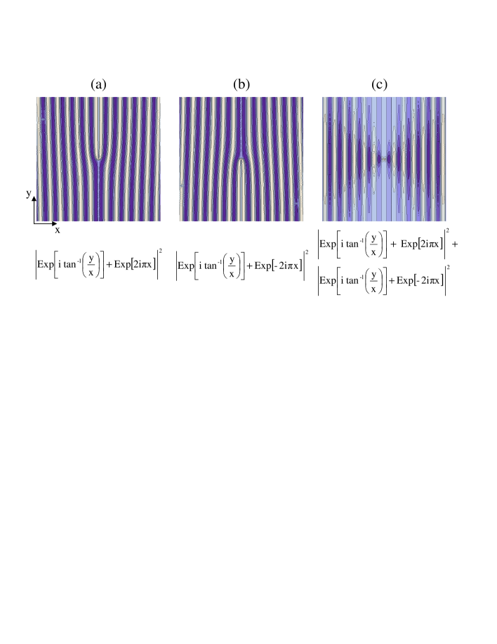
Figure 60: Holographic patterns corresponding to (a) chirality $+1$ of the reference, (b) chirality $-1$ of the reference and (c) sum of the previous two cases.

The shape of such kind of holograms ”is characterized by nearly parallel” fringes, ”except for a forking pattern in the vicinity of the core” SAKS , as shown in the example of Fig. 60. For chirality $+1$ (bottom case on the right of Fig. 59, corresponding to case $(a)$ in Fig. 60) the forking pattern will be directed upwards, for chirality $-1$ (upper case on the right of Fig. 59, corresponding to case $(b)$ in Fig. 60), downwards. When we have simultaneous overlapping of the two reference pulses with the Optical replica pulse (center case on the right of Fig. 59, corresponding to case $(c)$ in Fig. 60) we have a combination of two forking patterns one upwards and the other downwards.

It remains to be discussed whether the separation of the holographic fringes is enough to guarantee distinguishable patterns. The separation between the fringes depends on the transverse offset of the reference source relative to the object. When the offset of the reference source increases up to about $3\sigma$, $\sigma$ being the rms transverse electron bunch dimension, the fringes will be separated of a distance proportional to $1/3\sigma$, which is much larger compared to $1/(\gamma\lambdabar)$. As a result, for the first fringe we will obtain a fork which is well distinguishable, meaning that it does not overlap with the bunch structure and it is not influenced by the structure of the single electron pattern.

We can speculate that computerized analysis will easily distinguish among these three kinds of events, solving the problem of identifying the position of the slice within the bunch. There are many advantages related to the application of this technique. In fact, it avoids complications like the need for ITA, it does not require a-priori information about the electron bunch structure (i.e. can be used to measure ultra-short bunches) and it does not require synchronization.

7.4 HOTRI technique to provide a full 3D image of individual, arbitrary electron bunches

In this Section we introduce a novel technique to characterize the 3D structure of the electron bunch. This technique combines multiple-reference FTH (Section 7.2.2) and time-gated FTH (Section 7.3.4) methods. The fact that multiple-reference FTH may be naturally used for time-resolved experiments was first discussed in a concept presented in SCH2 .

Multiple-reference FTH can allow us to simultaneously record images of different slices of the electron bunch, thus providing a 3D image of a single electron bunch. Our idea is to vary the time-delay of the reference sources. Each reference source is a small disk with high reflectivity, and the distance from the reference scatter to the membrane is varied in order to create a time-delay between reference wave and OTR object wave, Fig. 61, left. As a result, once the hologram is processed, different reconstructed object images will correspond to different slices with given time-delays along the electron bunch, Fig. 61, right.

Figure 61: Membrane for time-resolved FTH with reference scatters (left) and reconstructed holographic images of electron bunch slices (right).

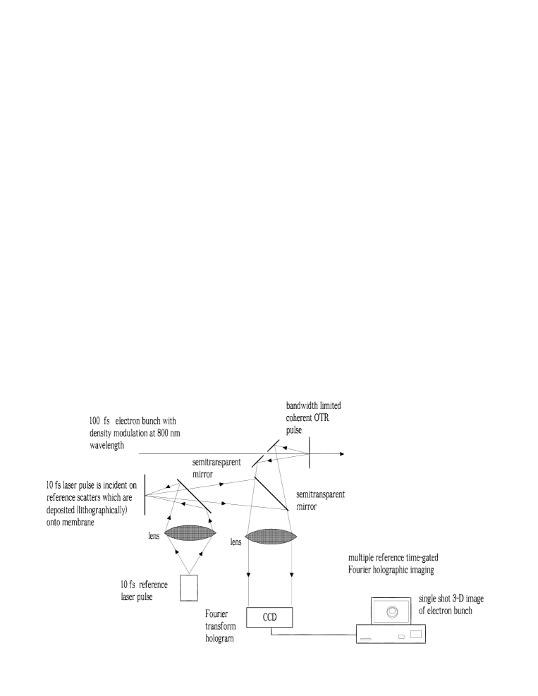
Figure 62: 3D electron bunch structure monitor by use of the HOTRI technique.

From the measurement using the setup shown in Fig. 62, we can make a movie (five frames with $10$ fs exposure-time and $50$ THz frame-rate) of the electron bunch propagating through the OTR screen, showing the electron density distribution against space and time. We named this novel technique Holography Optical Time Resolved Imaging (HOTRI).

8 Sensitivity to the energy chirp of the electron bunch

As we mentioned above, some coherent imaging techniques take advantage of the fact that the test pulse is bandwidth-limited. In this Section we will discuss what conditions should be met for the optical replica pulse to be considered bandwidth-limited, and what is the impact of a phase-chirp on the different techniques proposed in this work.

In Section 2 we discussed the impact of self-interactions on the optical replica. We demonstrated that, in practical cases of interest, self-interactions effects and energy-spread influence can be neglected, and the amplitude of the bunching can be considered uniform along the bunch. This is sufficient to produce an optical replica of the electron bunch, that is a radiation pulse whose electric field amplitude is a replica of the charge density distribution of the electron bunch. The optical replica pulse can be used to characterize the longitudinal bunch profile of the electron bunch ORSS with the FROG technique.

It should be remarked, however, that the bunch compression procedure introduces an energy chirp in the electron beam after the magnetic chicane BC2 in the case of the European XFEL, Fig. 5. This chirp introduces, as it will be discussed below, a distortion into the phase of the bunching which is not important for the ORS setup as concerns peak-current measurements, but is important when dealing with electron bunch imaging. A comprehensive analysis of the evolution of the longitudinal phase space after compression, including nearly all important physical effects (space charge interactions, Coherent Synchrotron Radiation (CSR), shape variation, resistive walls) is given in MART . The longitudinal phase-space of the electron bunch just after the magnetic compressor BC2, taken from MART is reproduced in Fig. 63.

Figure 63: The foreseen longitudinal phase-space distribution of electrons after the magnetic compressor BC2 at the European XFEL, extracted from MART .

The energy chirp shown in Fig. 63 is due to a combination of different effects. In fact, energy chirp is intrinsically introduced in the framework of a single-particle dynamics during the bunch compression procedure, but it is modified by the presence of other wakefields. Moreover, as noted in MART , the bunch formation system is composed by several chicanes, which complicates furthermore the situation. A qualitatively similar conclusion can be found in simulations for LCLS (see the study on longitudinal phase-space in LCLS ).

The measurement of the longitudinal bunch profile by FROG is insensitive to the presence of the energy chirp and, better, as shown in SLCH , the ORS can be used to measure the energy chirp. In fact, a FROG device can measure the phase of the optical replica, and the phase is strongly related to the energy chirp by

$$\delta\phi=\frac{R_{56}}{\lambdabar_{m}}\frac{\delta\gamma}{\gamma}~{}.$$ (156)

However, the phase chirp of the optical replica pulse is, in its turn, related to whether or not the optical replica pulse is bandwidth limited.

For a bandwidth-limited pulse of duration $\tau_{p}$ and bandwidth $\Delta\omega$ one has $\Delta\omega\tau_{p}\sim 1$. This implies that $\Delta\omega/\omega\sim(\omega\tau_{p})^{-1}$. Also, for a bandwidth-limited pulse, one should have a constant phase i.e., from a practical viewpoint, a phase-shift smaller than a radian along the pulse. A phase-chirp linear in time corresponds to a shift in the carrier frequency. One can account for such a chirp by introducing an effective carrier frequency. Thus, we will neglect the linear phase-chirp and account for the non-linear phase-chirp only. We may restate the condition above, requiring that the non-linear chirp should be sufficiently small, and the phase distortion across the pulse should be smaller than a radian.

Here we consider the low energy case of $2$ GeV after the second bunch compressor, where the longitudinal phase-space is depicted in Fig. 63. The value of the momentum compaction factor is that of the ORS dispersion section, i.e. $R_{56}\simeq 50~{}\mu$m. With the help of Eq. (156), one can see that a phase shift $\delta\phi$ of a radian corresponds to an energy shift of about $\Delta\gamma\sim 5$ MeV along the pulse. Considering the European XFEL case, one should extract from the large linear chirp Fig. 63, the non-linear energy chirp component. A quick estimation shows that the non-linear component of the chirp is in the order of $2\div 3$ MeV per bunch length, yielding a phase shift smaller than a radian. There is some room to optimize the situation by increasing the energy modulation introduced by the seed laser, increasing the energy in the seed laser pulse and subsequently decreasing the $R_{56}$ parameter in Eq. (156) of a factor $2\div 3$.

It should be noted that the large chirp shown in Fig. 63 is introduced ad hoc at the European XFEL (and at LCLS too) in order to diminish CSR effects in the chicane. Additionally this also allows to compensate for the linear component of the energy chirp introduced by wakefields after the bunch formation system, which has opposite slope. In several situations of interest, the non-linear component of the chirp can be smaller at the end of the bunch formation system.

Having said this, it is interesting to discuss which techniques presented in this paper are influenced by the energy chirp of the electron beam, and which are not.

First, let us consider methods that are not influenced. As we have seen in Section 5, direct (coherent) imaging without spectral filter allows one to record the integral of the squared modulus of the optical replica pulse, i.e. a quadratic projection. In this case, any phase deviation along the optical replica pulse is irrelevant. In fact, energy chirp only introduces a phase perturbation which depends on time and not on transverse coordinates, at least within a single-particle dynamics approximation in the bunch-formation system.

Also techniques based on the a-priori use of information from independent FROG measurements work, without modification, with and without chirp. This is the case when we combine real and reciprocal space spectrometers, Fig. 40, and when we consider frequency-gated FTH, Fig. 51. Other techniques which are completely insensitive to energy chirp are spatio-temporal FTH, Fig. 52 and HOTRI, Fig. 62 and, more in general, all time-gated FTH techniques. This follows from the short duration of the reference pulse in all these cases, which is $10$ fs long and has a bandwidth of about $100$ nm. In fact, the non-linear energy chirp necessary to significantly perturb the operation of time-resolved techniques based on such kind of reference pulses can be estimated to be about $100$ MeV, which is far from the design parameters of the European XFEL and LCLS. As a result, direct (coherent) imaging without spectral filter, techniques based on independent FROG measurements, the spatio-temporal FTH method and all time-gated FTH techniques are insensitive to energy chirp.

Second, there are techniques that are influenced by the presence of energy chirp, but that may be easily modified to account for such presence. These are schemes operating in the frequency domain in the 3D imaging mode, i.e. the multishot measurement method based on the use of the projection algorithm, Fig. 41, and FRODI, Fig. 42. In order to account for the effects of the energy chirp, in these cases we can make use of the knowledge about the phase deviation along the optical replica pulse as measured by FROG. This requires modification of the technique, because it implies an extra FROG measurement. Note that the required information is automatically available if we perform peak-current profile measurements.

Once the phase along the optical replica pulse is known, we can use it e.g. in the reconstruction of 2D traces for FRODI. Consider, for the sake of illustration, the $(x,t)$ projection. If we assume that the optical pulse is bandwidth-limited, its phase is constant, and $\rho_{0}$ and $a_{f}$ are real and positive (see Eq. (95)), i.e. one can talk about the slowly varying real and positive envelope of the pulse. If, instead, the optical pulse is not bandwidth limited, one has $a_{f}=a_{0}\exp[i\phi(t)]$ with $a_{0}$ constant and $\phi(t)$ a non-zero phase due to energy chirp within the electron bunch.

Therefore, when the energy chirp is negligible, the envelope of the optical replica pulse is an exact replica of $\rho_{0}(t,x,y)$, i.e. of the electron density distribution, which is real and nonnegative. As seen before, this is enough to guarantee unique reconstruction of the object. The fact that the optical replica pulse envelope is real and nonnegative actually amounts to complete information about the phase of the pulse envelope, which is just constant. When non-negligible energy chirp is present, the pulse envelope is no more real, but the phase along the $t$ axis is nevertheless fully determined by the FROG measurements, and this is enough to guarantee reconstruction. This allows to reconstruct any arbitrary projection $(x^{\prime},t)$, where $x^{\prime}$ is rotated of an arbitrary angle with respect to $x$ in the $(x,y)$ plane, but not the $(x,y)$ trace. Anyway, if a sufficient number of $(x^{\prime},t)$ traces are known, this information is enough for reconstruction. Note that the 3D optical replica pulse in the space-time domain can now be reconstructed as a cube of complex-valued data. The amplitude is proportional to $\rho_{0}(t,x,y)$.

Finally, third, all other techniques presented in this work, including direct (coherent) imaging with spectral filter, Fig. 27, linear projection diffraction imaging, Fig. 33, and FTH imaging of linear projection, Fig. 46, can operate only with a bandwidth-limited optical replica pulse. Note that when we extend these techniques to 3D reconstruction methods we can easily overcome the energy-chirp problem. However, when we deal with single $(x,y)$ projection measurement only, like in Fig. 27, Fig. 33 and Fig. 46, this is not possible anymore and one should take care that the energy chirp is actually negligible.

9 Conclusions

The study presented in this work opens up a novel field in high-energy, ultrashort electron beam diagnostic methods, based on the use of coherent Optical Transition Radiation (OTR) for 3D imaging of an ultrashort electron bunch by means of the Optical Replica Synthesizer (ORS) ORSS .

The ORS technique was proposed as an attempt to solve a very challenging problem, namely the longitudinal electron bunch diagnostics, by producing a 1D optical replica radiation pulse, thus reducing the electron bunch characterization problem to the 1D optical pulse characterization problem. The ORS performs longitudinal diagnostics of ultrarelativistic, ultrashort electron bunches in two steps. First, an optical replica of the electron bunch is prepared. Second, 1D characterization of the electron bunch is performed by a femtosecond oscilloscope. For this purpose the ORS setup makes use of a commercially available Frequency-Resolved Optical Gating (FROG) device. The availability of methods and instrumentation for measuring ultrashort optical pulses constitutes the main advantage of using an optical replica compared to other diagnostics schemes.

In the case of 3D characterization of an electron bunch we demonstrated that the same approach can be realized. In other words, the 3D imaging of an electron bunch with spatio-temporal coupling can be reduced to 3D characterization of an optical pulse with spatio-temporal coupling. However, the 3D problem has a different status compared to its 1D counterpart. In fact, the 3D problem was formulated only recently, and no commercial devices are yet available. This does not mean that the schemes discussed in this work constitute a challenge as concerns their technical realization. The 3D problem has a number of possible solutions, and this explains why some of the techniques proposed here (FRODI, HOTRI) are completely original. Note that our formulation of the 3D problem is less general than the one addressed by the optical community. In our case of interest, the optical pulse is not arbitrary, but being the optical replica of an electron bunch, has a duration of about $100$ fs and has specific constraints like the bandwidth limit, or in more general cases, a phase which is a function of time only. This opens up the possibility to use some approaches, as Fourier Transform Holography (FTH) with reference source and its variations, which cannot be applied for an arbitrary pulse.

We proposed to use coherent OTR as the source of radiation for the optical replica pulse. In the case of coherent OTR we can take advantage of the large number of photons and of the coherent properties of the radiation pulse. We developed schemes based on direct coherent OTR imaging, diffractive imaging, FTH, and a combination of these techniques. In particular, novel techniques like FRODI and HOTRI allow for the 3D characterization of ultrashort electron bunches by use of single and multishot measurements.

We proposed to exploit the highly-developed software algorithms for Diffractive Imaging and Fourier Transform Holography. Reconstruction of 3D images in real space-time domain can be based on methods like the Gerchberg-Saxton algorithm, the Fineup algorithm or their generalizations. Moreover, similarly to the ORS setup, we proposed to make use of the large selection of commercially available instrumentation for optical pulse diagnostics. Performing diagnostics in the range of visible optics will greatly simplify a choice of optical elements or their manufacturing. Also, ultrashort, up to $10$ fs, optical laser sources with any state of polarization are available as a reference sources. The same approach, to use already highly-developed devices, is proposed when considering 3D-imaging methods in the 3D Fourier domain. For this kind of applications there is a need for optical systems capable of forming high-resolution images at different wavelengths. Imaging spectrometers are instruments capable of providing this functionality. There are two types of imaging spectrometers. One type is based on the use of a plurality of bandpass filters to measure a 3D data cube in the 3D Fourier domain for different frequencies. A second type is based on the use of a dispersive element, and it is particularly suitable for single shot 3D measurements.

Due to the users’ needs, future XFELs will operate with shorter and shorter electron bunches. Our proposed diagnostic techniques have the potential for extensions from the $100$-fs time scale, which we discussed here, to the $10$-fs time scale of electron bunch duration by straightforward rescaling to shorter wavelengths. Exploitation of shorter wavelengths is possible because our setups are based on linear optical elements only. The shortest possible wavelength compatible with glass optics is about $200$ nm, which corresponds to the fourth harmonic of a Ti:Sa laser. Using particular geometries, FROG devices can operate in this range as well FROG .

We regard the concepts presented here, based on the combination of ORS with coherent OTR imager setups, as the start of a novel direction in diagnostic methods. Therefore, the present work should not be considered as comprehensive of all foreseeable applications. On the contrary, we hope that our work will stimulate interest and open the door to many new possibilities for ultra-fast electron bunch diagnostics.

10 Acknowledgements

We thank our colleagues Dirk Noelle, Harald Redlin and William Schlotter for useful discussions, Massimo Altarelli, Reinhard Brinkmann and Edgar Weckert for their interest in this work.

References

- [1] J. Arthur et al. Linac Coherent Light Source (LCLS). Conceptual Design Report, SLAC-R593, Stanford (2002) (See also http://www-ssrl.slac.stanford.edu/lcls/cdr).
- [2] Tanaka, T. & Shintake, T. (Eds.): SCSS X-FEL Conceptual Design Report. Riken Harima Institute, Hyogo, Japan, 2005 (see also http://www-xfel.spring8.or.jp).
- [3] M. Altarelli et al. (Eds.), XFEL: The European X-Ray Free-Electron Laser. Technical Design Report, DESY 2006-097, DESY, Hamburg (2006) (See also http://xfel.desy.de).
- [4] A.M. Kondratenko and E.L. Saldin, Part. Accelerators 10 (1980) 207.
- [5] Ya.S. Derbenev, A.M. Kondratenko and E.L. Saldin, Nucl. Instrum. and Methods 193 (1982) 415.
- [6] R. Bonifacio, C. Pellegrini and L. Narducci, Opt. Commun. 50 (1984) 373.
- [7] J.B. Murphy and C. Pellegrini, Nucl. Instrum. and Methods A 237 (1985) 159.
- [8] E. Saldin, E. Schneidmiller and M. Yurkov, Nucl. Instrum. and Methods 539, 3 (2005) 499.
- [9] R. Trebino, ”Frequency-resolved optical gating: the measurement of ultrashort laser pulses”, Boston, Kluwer Academic Publishers (2002).
- [10] A. Angelova et al., Phys. Rev. ST Accel. Beams 11 (2008) 070702.
- [11] A. Angelova et al., TUPC114, Proceedings of EPAC 2008, Genova, Italy (2008) 1332.
- [12] G. Geloni, E. Saldin, E. Schneidmiller and M. Yurkov, Opt. Commun. 281 (2008) 3762.
- [13] G. Geloni, E. Saldin, E. Schneidmiller and M. Yurkov, Phys. Rev. ST AB 11 (2008) 120701.
- [14] F. Bragheri et al., Opt. Lett. 33, 24 (2008) 2952.
- [15] R.W. Gerchberg and W. Saxton, Optik 35 (1972) 237.
- [16] N. Abramson, Opt. Lett. 3, 4 (1978) 121.
- [17] P.L. Csonka, Part. Accel. 8 (1978) 225.
- [18] G. Geloni, E. Saldin, E. Schneidmiller and M. Yurkov, Nucl. Instrum. and Meth. in Phys. Res. A 583 (2007) 228.
- [19] H. Loos et al., Observation of Coherent Optical Transition Radiation in the LCLS Linac, SLAC-PUB-13395 (2008).
- [20] E. Saldin, E. Schneidmiller and M. Yurkov, Nucl. Instrum. and Methods in Phys. Res. A 528 (2004) 355.
- [21] V.L. Ginzburg and I. M. Frank, Soviet Phys. JETP 16 (1946) 15.
- [22] H. Wiedemann, Synchrotron Radiation, Springer Berlin, 2003.
- [23] G. Geloni, E. Saldin, E. Schneidmiller and M. Yurkov, ”Theory of Edge Radiation” DESY 08-118 (2008), http://arxiv.org/abs/0808.1846, submitted to Nucl. Instrum. and Methods in Phys. Res. A.
- [24] European XFEL Start-to-End Simulations, http://www.desy.de/xfel-beam/s2e/xfelv4.html (2006).
- [25] G. Geloni, E. Saldin, E. Schneidmiller and M. Yurkov, Optics Communications 276, 1 (2007) 167.
- [26] J. Jackson, Classical Electrodynamics, 3rd ed., Wiley, New York, 1999
- [27] J. Rosenzweig, G. Travish, A. Tremaine Nucl. Instr. and Methods A 365 (1995) 255.
- [28] Tremaine, et al, Phys. Rev. Letters 81 (1998) 5816.
- [29] A. Tremaine, et al, Nucl. Instrum. and Methods in Phys. Res. A 429 (1999) 209.
- [30] A. H. Lumpkin, et al., Phys. Rev. Lett. 86 (2001) 79.
- [31] A. H. Lumpkin, et al., Phys. Rev. Lett. 88 (2002) 23801.
- [32] A. H. Lumpkin, et al., Nucl. Instrum. and Methods in Phys. Res. A 507 (2003) 200.
- [33] A. H. Lumpkin, et al, Nucl. Instrum. and Methods in Phys. Res. A 528 (2004) 179.
- [34] B. Yang, A design report for the optical transition radiation imager for the LCLS undulator, LCLS-TN-05-21 (2005).
- [35] J. W. Goodman, Introduction to Fourier Optics, Mc Graw-Hill Book Company (1968).
- [36] P. Dumontet, Opt. Acta 2 (1955) 53.
- [37] D.A. Tichenor and J.W. Goodman, J. Opt. Soc. Am. 62 (2008) 293.
- [38] J.P. Mills and B.J. Thompson, J. Opt. Soc. Am. A, 3, 5, 694 (1986).
- [39] E. Brainis, C. Muldoon, L. Brandt and A. Kuhn, Optics Communications 282 (2009) 465.
- [40] M. Castellano and V.A. Verzilov, Spatial Rosolution in Optical Transition Radiation (OTR) beam diagnostics, LNF-98/017(P) (1998).
- [41] V.A. Lebedev, Nucl. Instrum. and Meth. in Phys. Res. A 372 (1996) 344.
- [42] R. Bakarat, J. Opt. Soc. Am. 52 (1962) 276.
- [43] G. Machavariani et al., Optics Communications 281 (2008) 732.
- [44] P.B. Phua, High power radially polarized light generated from photonic crystal segmented half-wave-plate, http://arxiv.org/abs/0710.4979v1 (2007)
- [45] S. G. Lipson, H. Lipson and D. S. Tannhauser, Optical Physics, Cambridge University press (1995).
- [46] M. Born and E. Wolf, ”Principles of Optics”, 5th ed., Pergamon, Oxford (1975).
- [47] J. R. Fineup, Appl. Optics, 21 (1982) 2758.
- [48] R. P. Millane, J. Opt. Soc. Am. A 7 (1990) 394.
- [49] J. R. Fineup, Appl. Optics 32 (1993) 1737.
- [50] J. R. Fineup and A. M. Kowalczyk, Opt. Soc. Am. A 7 (1990) 450.
- [51] P.R. Luke, J.V. Buske and R.G. Lyon, SIAM Review, 44, 2 (2002) 169.
- [52] G. W. Stroke and D. Falconer, Phys. Lett. 13 (1964) 306.
- [53] Z.S. Sacks et al. J. Opt. Soc. Am. B, 15, 8 (1998) 2226.
- [54] L-M. Stadler et al., Phys. Rev. Lett. 100 (2008) 245503.
- [55] W. F. Schlotter et. al., Appl. Phys. Lett. 89 (2006) 163112.
- [56] P. Gabolde and R. Trebino Optics Express 12, 19 (2004) 4223.
- [57] Y. T. Mazurenko, Appl. Phys. B 50, (1990) 101.
- [58] Y. T. Mazurenko, Opt. Eng. 31, (1992) 739.
- [59] A. M. Weiner and D.E. Leaird, OPt. Lett. 19, (1994) 123.
- [60] J. P. Geindre et al., Opt. Lett. 19 (1994) 1997.
- [61] T. Tanabe et al. J. Opt Soc. Am. B 19 (2002) 2795.
- [62] P. Gabolde and R. Trebino Optics Express 14, 23 (2006) 11460.
- [63] C. Dorrer, E. Kosik and I. Walmsley, Appl. Phys. B 74 (2002) S209.
- [64] A. Monmayrant, S. Gorza, P. Wasylczyk and I. Walmsley, Beyond the fringe: SPIDER - the anatomy of ultrashort laser pulses”, Photonik international 2007, (2007) 2.
- [65] Z. S. Sacks, D. Rozas, and G. A. Swartzlander Jr., J. Opt. Soc. Am. B, 15, 8 (1998) 2226.
- [66] W. F. Schlotter et. al., Opt. lett. 32 (2007) 21.
- [67] M. Dohlus, Modelling of space charge and CSR effects in bunch compression systems, in Proceedings of EPAC 2006, Edinburgh, Scotland, WEYFI01, (2006) 1897.
- [68] Y. Ding, Z. Huang and P. Emma, Integration of the optical replica ultrashort electron bunch diagnostics with the current-enhanced SASE in the LCLS, SLAC-PUB 12672 (2007).