Present Address: ]Department of Physics, Indian Institute of Technology Delhi, New Delhi 110 016, India

Electron transport across electrically switchable magnetic molecules

Abstract

We investigate the electron transport properties of a model magnetic molecule formed by two magnetic centers whose exchange coupling can be altered with a longitudinal electric field. In general we find a negative differential conductance at low temperatures originating from the different scattering amplitudes of the singlet and triplet states. More interestingly, when the molecule is strongly coupled to the leads and the potential drop at the magnetic centers is only weakly dependent on the magnetic configuration, we find that there is a critical voltage $V_{\mathrm{C}}$ at which the current becomes independent of the temperature. This corresponds to a peak in the low temperature current noise. In such limit we demonstrate that the quadratic current fluctuations are proportional to the product between the conductance fluctuations and the temperature.

An intriguing aspect of electronic transport is the interaction between the current electrons and the internal degrees of freedom of the conductor. Atomic positions and vibrations are certainly at research center-stage, electro-migration being the most obvious example of interplay between the current and the atoms motion. The situation becomes even more intriguing at the nanoscale, where quantized vibrations can be detected by measuring the electron current and its derivatives with respect to the applied bias. This is the principle of inelastic electron tunneling spectroscopy (IETS). Furthermore also the reverse effect is possible, namely one can control the atomic positions of a nano-object by exciting appropriately some vibrational modes. Current-induced chemical reactions cicrs and nano-catalysis nanocat on surfaces are among the most appealing potential applications of this field.

Equally important is the interplay between the electron current and the magnetic texture of a magnetic device. Such an interplay underpins the giant magnetoresistance effect gmr and its reverse, i.e. current induced magnetization dynamics spintorque . Considerably less investigated are the same phenomena at the atomic scale. This is mainly due to the intrinsic difficulties of both manipulating and detecting a few spins. In addition, magnetic excitations occur at energies lower than those involved in molecular vibrations, so that the measuring temperatures are often rather low. Still there are notable examples, such as ultra low temperature IETS of magnetic atoms on surfaces IBM and of two-probe devices incorporating single magnetic molecules WenMS .

A new exciting prospect for scaling down spin-dynamics to the atomic level may be given by the ability of manipulating the magnetic configuration of a molecule with an electric potential instead of an electric current. Electrically induced alteration of the exchange coupling has been already predicted for two-centers magnetic molecules ESCE and nanowires Angw , and it is essentially based on the fact that the Stark shift of a magnetic object may depend on its magnetic state. This effect can be a crucial ingredient for the physical implementation of quantum computing based on spins SMMQC ; AffronteNew .

An intriguing question is whether or not the dependance of the exchange coupling over an electrical potential in a magnetic molecule can be detected electrically. This is the goal of our letter where we investigate the current-voltage, $I$-$V$, curve of a two-terminal device incorporating a two-center magnetic molecule in which the exchange coupling changes with bias. Importantly we find that, in particular conditions of coupling between the molecule and the electrodes, there is a critical voltage $V_{\mathrm{C}}$ at which the current becomes independent of the temperature. This is accompanied by a negative differential conductance (NDC) at low temperature originating from the difference in scattering amplitude of the different spin-states of the molecule.

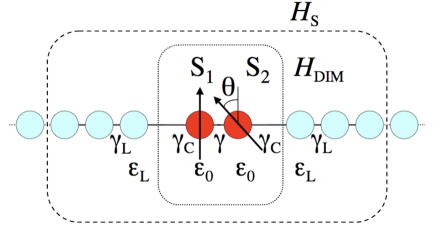
Figure 1: (Color on line) The model system investigated: a dimer of magnetic atoms (red), carrying respectively spin $S_{1}$ and $S_{2}$, is attached to two 1D non-magnetic electrodes (light blue). The Hamiltonian for the dimer is $H_{\mathrm{DIM}}$. The scattering region (dashed box) includes the dimer and six atoms of the electrodes and it is described by the Hamiltonian matrix $H_{\mathrm{S}}$.

In figure 1 we show the simple model system investigated, which comprises a di-atomic magnetic molecule sandwiched between two one-dimensional non-magnetic electrodes. The system is described by the $s$-$d$ model Yosida96 ; Maria , where spin of the current carrying $s$-electrons is exchange-coupled to the local spins $S_{1}$ and $S_{2}$ ($d$) of the two atoms in the dimer. $S_{1}$ and $S_{2}$ are treated as classical variables and their orientation determines the scattering potential for the $s$-electrons. These are described by a tight-binding Hamiltonian with a single $s$-orbital per site at half-filling. The on-site energy and hopping integral in the electrodes are $\epsilon_{\mathrm{L}}=2$ eV and $\gamma_{\mathrm{L}}=-2$ eV, a choice which maintains the system far from the van Hoof singularities at any voltage investigated. No local spins are present in the electrodes so that their electronic structure is not spin-polarized. The Hamiltonian of the dimer is

$$H_{\mathrm{DIM}}=\sum_{\alpha\beta}\sum_{i}^{1,2}h_{i}^{\alpha\beta}c_{i}^{\alpha\dagger}c_{i}^{\beta}+\sum_{\sigma}\gamma(c_{1}^{\sigma\dagger}c_{2}^{\sigma}+c_{2}^{\sigma\dagger}c_{1}^{\sigma})\>,$$ (1)

where $h_{i}^{\alpha\beta}$ is the on-site Hamiltonian matrix of the $i$-th atom of the dimer, $\gamma$ is the hopping parameter and $c_{i}^{\sigma\dagger}$ ($c_{i}^{\sigma}$) is the creation (annihilation) operator for an electron with spin $\sigma$ ($\uparrow,\downarrow$) at the site $i$. We have defined $h_{i}^{\alpha\beta}=[\epsilon_{0}+U(\rho_{i}-\rho_{0})]\delta_{\alpha\beta}-J_{\mathrm{sd}}\vec{S}_{i}\cdot\left({\vec{\sigma}}\right)_{\alpha\beta}$, where ${\vec{\sigma}}$ are the Pauli matrices, $\rho_{i}$ is the total occupation of $i$-th site, $\rho_{0}=1$ is the site occupation in the neutral configuration, $U=1$ eV is the atomic charging energy and $J_{\mathrm{sd}}=2$ eV is the exchange parameter between the $s$-electrons and the local spins. In our calculations we consider $\epsilon_{0}=2$ eV, $\gamma=-0.1$ eV, $|\vec{S}_{i}|=1$. In absence of spin-orbit interaction and spin-polarization of the electrodes the scattering potential is determined only by the mutual angle, $\theta$, between the two local spins. Finally, the dimer and the electrodes are coupled by the hopping integral $\gamma_{\mathrm{C}}$. In particular we explore the two cases in which $\gamma_{\mathrm{C}}=1/4\gamma_{\mathrm{L}}$ and $\gamma_{\mathrm{C}}=1/2\gamma_{\mathrm{L}}$. These parameters are only illustrative and have been chosen in order to maximize the difference in conductance between different spin-states of the molecule ($\theta=0$ vs $\theta=\pi$).

The non-equilibrium Green function method Datta applied to our tight-binding Hamiltonian Alex is used to calculate the transport properties. The central quantity is the retarded Green’s function of the scattering region

$$G(E)=\lim_{\eta\to 0+}\left[(E+i\eta)-H_{\mathrm{DIM}}-\Sigma_{\mathrm{L}}-\Sigma_{\mathrm{R}}\right]^{-1}\>,$$ (2)

where $E$ is the energy, $H_{\mathrm{S}}$ is the Hamiltonian matrix of the scattering region and $\Sigma_{\mathrm{L}}$ ($\Sigma_{\mathrm{R}}$) is the self-energy of the left- (right-) hand side electrode. This latter describes the interaction between the scattering region, which includes the dimer and 6 atoms of the electrodes (see Fig. 1), and the electrodes. $G(E)$ enters in a self-consistent procedure to evaluate the stationary occupation of the scattering region and once convergence is achieved the two-probe microscopic current, $i(V)$, at the voltage $V$ is extracted from the Landauer formula Alex .

Since at any given temperature the angle between the magnetic moments in the dimer fluctuates, for any microscopic quantity $q$ we can define its macroscopic counterpart, $Q$, as the thermal average over all the possible angles

$$Q(V)=\langle q(V)\rangle=\frac{\int_{{\cal E}_{\mathrm{min}}}^{{\cal E}_{\mathrm{max}}}q(\theta,V)\mathrm{e}^{-\frac{{\cal E}_{12}}{k_{\mathrm{B}}T}}\,\mathrm{d}{\cal E}}{\int_{{\cal E}_{\mathrm{min}}}^{{\cal E}_{\mathrm{max}}}\mathrm{e}^{-\frac{{\cal E}_{12}}{k_{\mathrm{B}}T}}\,\mathrm{d}{\cal E}}\>,$$ (3)

thus that if $q=i$ one obtains the macroscopic current, $I$. Here ${\cal E}_{12}$ is the dimer magnetic energy, which writes

$${\cal E}_{12}=-J_{\mathrm{dd}}\cos\theta\>,\;\;\;\;\;\;\;J_{\mathrm{dd}}=a+b\>v_{\mathrm{d}}^{2}(\theta,V)\>,$$ (4)

and ${\cal E}_{\mathrm{min}}$ (${\cal E}_{\mathrm{max}}$) is its minimum (maximum) value. In the equations (4) above $J_{\mathrm{dd}}$ is the exchange energy between the two spins, which in turns is a quadratic function of the electrical potential difference between them, $v_{\mathrm{d}}$. This latter is an intrinsic function of both $V$ and $\theta$. Finally the constants $a$ and $b$ are fixed to the values of $a=0.001$ eV and $b=-0.8$ eV/V². Note that the functional dependance of $J_{\mathrm{dd}}$ over $v_{\mathrm{d}}$ implies a critical voltage at which the exchange energy changes sign, i.e. the magnetic coupling turns from ferromagnetic to antiferromagneticESCE ; Angw .

We begin our analysis by investigating the microscopic quantities, i.e. the current $i(V,\theta)$ and the dimer internal potential drop $v_{\mathrm{d}}$. In Fig. 2 we present, for both choices of coupling $\gamma_{\mathrm{C}}$, $i$-$\theta$ for different voltages and $v_{\mathrm{d}}$-$V$ for different angles $\theta$. In the case of $\gamma_{\mathrm{C}}=1/4\gamma_{\mathrm{L}}$ the current varies as $i(V,\theta)\sim[i_{0}+i_{1}\cos\theta]V$, with $i_{0}$ and $i_{1}$ two constants. At the same time $v_{\mathrm{d}}$ is only weakly dependent on the internal spin configuration, i.e. the $v_{\mathrm{d}}$-$V$ curve changes little with the angle $\theta$ [Fig. 2(b)]. In contrast for $\gamma_{\mathrm{C}}=1/2\gamma_{\mathrm{L}}$ the current peaks at approximately $\theta=\pi/2$ with both the parallel and antiparallel configurations being low conducting. Again the amplitude of the current variation over $\theta$ increases with bias, although only moderately in this case. Furthermore for this situation $v_{\mathrm{d}}$, which is still linear with $V$, is rather sensitive to the angle between the two spins. These differences affect dramatically the macroscopic current, $I$, that we calculate next.

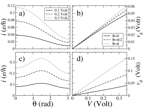
Figure 2: Microscopic transport quantities. The microscopic current, $i$, as a function of the angle, $\theta$, is shown in panels (a) and (c) for different voltages $V$. Panel (b) and (d) show the internal potential drop, $v_{\mathrm{d}}$, as a function of the external bias and for different angles. Panels (a) and (b) are for $\gamma_{\mathrm{C}}=1/4\gamma_{\mathrm{L}}$, while (c) and (d) are for $\gamma_{\mathrm{C}}=1/2\gamma_{\mathrm{L}}$.

The macroscopic $I$-$V$ curves for the two cases are presented in the panels (a) and (c) of Fig. 3, while the panels (b) and (d) report the current quadratic fluctuations $\Delta I=\sqrt{\langle i^{2}\rangle-I^{2}}$ still as a function of bias. In all cases we study the electrical response in the temperature range 1-15 K. The most interesting behaviour is found for $\gamma_{\mathrm{C}}=1/4\gamma_{\mathrm{L}}$, from which we start our discussion.

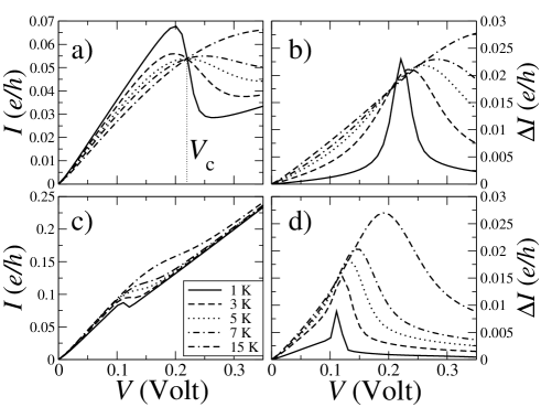
Figure 3: Macroscopic transport quantities. The $I$-$V$ curves are presented in panels (a) and (c), while panels (b) and (d) display the current quadratic fluctuations $\Delta I=\sqrt{\langle i^{2}\rangle-I^{2}}$ as a function of bias $V$. Panels (a) and (b) are for $\gamma_{\mathrm{C}}=1/4\gamma_{\mathrm{L}}$, while (c) and (d) are for $\gamma_{\mathrm{C}}=1/2\gamma_{\mathrm{L}}$. Note that in (a) there is a critical voltage $V_{\mathrm{C}}$ at which the current becomes independent of the temperature.

Figure 3(a) reveals two remarkable features. First we note that there is a pronounced NDC at about 0.2 Volt, which is well evident at 1 K, it weakens as the temperature increases and finally disappears at 15 K. Interestingly the scaling of the electrical current with the temperature is opposite at the two sides of the NDC: it decreases as the temperature is enhanced before the NDC while it grows with $T$ for voltages just after the NDC. The same NDC is present also in the case of stronger coupling with the leads [$\gamma_{\mathrm{C}}=1/2\gamma_{\mathrm{L}}$, Fig. 3(c)] at the somewhat lower voltage of about 0.1 Volt. In this case however the NDC is much less pronounced and disappears already at 3 K.

The second and most striking feature of Fig. 3(a) is the presence of a critical voltage, $V_{\mathrm{C}}$, at which the current becomes independent of the temperature. Such a voltage is in the vicinity of the NDC and correlates well with the peak in the current quadratic fluctuations [Fig. 3(b)] at low temperature. Note that this second feature is absent in the case of strong coupling to the leads.

All these aspects can be easily understood by relating the microscopic quantities of Fig. 2 with the average of equation (3). Let us consider the case of $\gamma_{\mathrm{C}}=1/4\gamma_{\mathrm{L}}$ first. In general the macroscopic current $I(V)$ is determined by the microscopic currents $i(V,\theta)$ of those configurations in which the system spends most of the time. The equations (4) tell us that the ferromagnetic configuration is energetically favorable at low bias, while it is the antiferromagnetic to dominate at higher voltages (for $v_{\mathrm{d}}$ larger than $\pm\sqrt{-a/b}$). This means that as the external bias increases the average current becomes progressively dominated by antiferromagnetic configurations to the expenses of the ferromagnetic ones. Since the microscopic current for $\theta=\pi$ is always considerably smaller than that for $\theta=0$ [see Fig. 2(a)], this results in a decrease of the macroscopic current as a function of bias, i.e. in the NDC. Note that this particular NDC is not of microscopic electronic origin since the microscopic currents $i(V,\theta)$ are monotonic in $V$ for every $\theta$.

The fact that the exchange coupling changes sign as a function of the bias produces the second important feature in the macroscopic $I$-$V$ curve. In fact when the potential drop between the two magnetic atoms is $v_{\mathrm{d}}=\pm\sqrt{-a/b}$, then the parallel and antiparallel configurations of the magnetic molecule become energetically degenerate. This means that now no magnetic energy scale enters into the problem and the system spends an equal amount of time in any spin configurations regardless of the temperature. In general $v_{\mathrm{d}}$ is proportional to the external bias $V$. Therfore one expects the existence of a universal external bias $V_{\mathrm{C}}=V[{\cal E}_{12}(v_{\mathrm{d}})=0]$ such that ${\cal E}_{12}=0$ and the macroscopic currents becomes independent of the temperature, as indeed demonstrated in Fig. 3(a). However there is a second condition for this to happen, i.e. $v_{\mathrm{d}}$ should be independent of the angle $\theta$. This is not satisfied for $\gamma_{\mathrm{C}}=1/2\gamma_{\mathrm{L}}$ [see Fig. 2(d)] and as a consequence the $I$-$V$ curves remain temperature dependent at any bias.

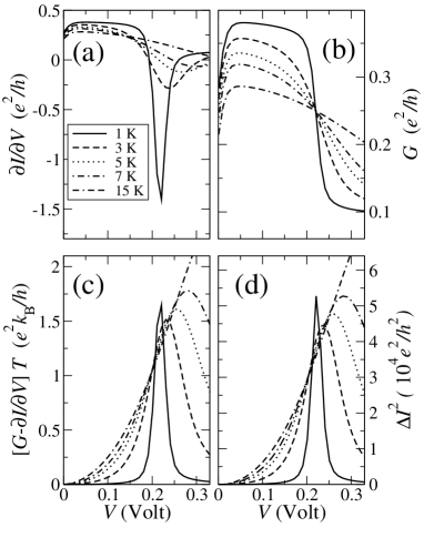
Figure 4: Differential conductance calculated as (a) the derivative of the macroscopic current, $I$, with respect to the bias or as the (b) thermal average, $G$, of the microscopic conductance. In panel (c) we show the product of $(G-\partial I/\partial V)$ with the temperature $T$, as a function of bias. Results are presented for $\gamma_{\mathrm{C}}=1/4\gamma_{\mathrm{L}}$. Note that $[G-\partial I/\partial V]T$ is proportional to the square of the current quadratic fluctuations $\Delta I^{2}$ [panel (d)] of figure 3(b).

From our discussion it is now clear that if $v_{\mathrm{d}}$ is proportional to $V$ and weakly dependent on $\theta$, then there will be a critical voltage $V_{\mathrm{C}}$ at which any macroscopic quantity becomes temperature independent. Figure 3(a) illustrates this feature for the current and the same is demonstrated in Fig. 4(b) for the conductance $G=\left\langle\frac{\partial i}{\partial V}\right\rangle$. Interestingly one can also adopt a different definition for the macroscopic conductance, namely that of the bias derivative of the macroscopic current $\partial I/\partial V$. Such a quantity is presented in Fig. 4(a) and as expected it appears sensibly different from $G$. Interestingly both $G$ and $\partial I/\partial V$ are, in principle, accessible from experiments, and one may wonder whether some general conclusions can be taken by measuring the two quantities independently.

In general, by taking the equation (3) and formally deriving $Q$ with respect to the bias $V$ we find

$$\left[\left\langle\frac{\partial q}{\partial V}\right\rangle-\frac{\partial Q}{\partial V}\right]k_{\mathrm{B}}T=\left\langle q\>\frac{\partial{\cal E}_{12}}{\partial V}\right\rangle-Q\left\langle\frac{\partial{\cal E}_{12}}{\partial V}\right\rangle\>,$$ (5)

where $k_{\mathrm{B}}$ is the Boltzman constant. If one now considers $q=i$ then the equation (5) establishes a general relation between the conductance fluctuations and the correlation function between the current and the magnetic energy. Such a relation is drastically simplified when the microscopic current has the typical spin-valve dependence $i(V,\theta)\sim[i_{0}+i_{1}\cos\theta]V$ and $v_{\mathrm{d}}$ is linear with $V$. In this situation (encountered here for $\gamma_{\mathrm{C}}=1/4\gamma_{\mathrm{L}}$) one finds

$$\left[G-\frac{\partial I}{\partial V}\right]k_{\mathrm{B}}T\propto\>\Delta I^{2}\>,$$ (6)

i.e. that the conductance fluctuations rescaled by the temperature are proportional to the squared current fluctuations. A numerical proof of such a relation is provided in the panels (c) and (d) of figure 4.

In conclusion we have investigated the temperature-dependent electronic transport through a model diatomic magnetic molecule, in which the exchange coupling between the two magnetic centers is a function of the bias. This presents two remarkable characteristics. First, if the potential drop between the two magnetic centers is only weakly dependent on the angle between their magnetic moments and it is linear in $V$, then there is a critical voltage $V_{\mathrm{C}}$ at which the macroscopic current becomes temperature independent. Secondly, if in addition the microscopic current has a form $i(V,\theta)\sim[i_{0}+i_{1}\cos\theta]V$, then there is a universal relation between the temperature-rescaled conductance fluctuations and the quadratic current fluctuations. Both these effects are a unique fingerprint of the dependance of the magnetic energy upon an external bias and can be used as a tool for detecting such a dependence.

This work is funded by Science Foundation of Ireland. We thank Maria Stamenova and Chaitanya Das Pemmaraju for helping with the numerical implementation and Tchavadar Todorov for useful discussion.

References

- (1) S. Katano, Y. Kim, M. Hori, M. Trenary and M. Kawai, Science 316, 1883 (2007).
- (2) B.J. McIntyre, M. Salmeron and G.A. Somorjai, Science 265, 1415 (1994).
- (3) M.N. Baibich et al., Phys. Rev. Lett. 61 2472 (1988; G. Binasch, P. Grünberg, F. Saurenbach and W. Zinn, Phys. Rev. B 39, 4828 (1989).
- (4) J. Slonczewski, J. Magn. Magn. Mater. 159, L1 (1996).
- (5) C.F. Hirjibehedin, C.-Y. Lin, A.F. Otte, M. Ternes, C.P. Lutz, B.A. Jones and A.J. Heinrich, Science 317, 1199 (2007).
- (6) L. Bogani and W. Wernsdorfer, Nature Materials 7, 179 (2008).
- (7) N. Baadji, M. Piacenza, T. Tugsuz, F. Della Sala, G. Maruccio and S. Sanvito, preprint.
- (8) M. Diefenbach and K.S. Kim, Angew. Chem. Int. Ed. 46, 7640 (2007).
- (9) J. Lehmann, A. Gaita-Ario, E. Coronado and D. Loss, Nature Nanotech. 2, 312(2007).
- (10) G.A. Timco et al., Nature Nanotechnology 4, 173 (2009).
- (11) K. Yosida, Theory of Magnetism, Springer-Verlag, 1996.
- (12) M. Stamenova, T.N. Todorov and S. Sanvito, Phys. Rev. B 77, 054439 (2008).
- (13) S. Datta, Electronic transport in Mesoscopic Systems, Cambridge University Press, 1995.
- (14) A.R. Rocha and S. Sanvito, Phys. Rev. B 70, 094406 (2004).