High-redshift obscured quasars: radio emission at sub-kiloparsec scales

Abstract

The radio properties of 11 obscured ‘radio-intermediate’ quasars at redshifts $z\mathrel{\hbox{\hbox to0.0pt{\hbox{\lower 2.0pt\hbox{$\sim$}}\hss}\raise 2.0pt\hbox{$>$}}}2$ have been investigated using the European Very-Long-Baseline-Interferometry Network (EVN) at 1.66 GHz. A sensitivity of $\sim$${\rm 25~{}\mu Jy~{}per~{}17\times 14~{}mas^{2}~{}beam}$  was achieved, and in 7 out of 11 sources unresolved radio emission was securely detected. The detected radio emission of each source accounts for $\sim 30-100$% of the total source flux density. The physical extent of this emission is $\mathrel{\hbox{\hbox to0.0pt{\hbox{\lower 2.0pt\hbox{$\sim$}}\hss}\raise 2.0pt\hbox{$<$}}}$ 150 pc, and the derived properties indicate that this emission originates from an active galactic nucleus (AGN). The missing flux density is difficult to account for by star-formation alone, so radio components associated with jets of physical size $\mathrel{\hbox{\hbox to0.0pt{\hbox{\lower 2.0pt\hbox{$\sim$}}\hss}\raise 2.0pt\hbox{$>$}}}$ 150 pc  and $\mathrel{\hbox{\hbox to0.0pt{\hbox{\lower 2.0pt\hbox{$\sim$}}\hss}\raise 2.0pt\hbox{$<$}}}40$ kpc are likely to be present in most of the sources. Amongst the observed sample steep, flat, gigahertz-peaked and compact-steep spectrum sources are all present. Hence, as well as extended and compact jets, examples of beamed jets are also inferred, suggesting that in these sources, the obscuration must be due to dust in the host galaxy, rather than the torus invoked by the unified schemes. Comparing the total to core ($\mathrel{\hbox{\hbox to0.0pt{\hbox{\lower 2.0pt\hbox{$\sim$}}\hss}\raise 2.0pt\hbox{$<$}}}$150 pc) radio luminosities of this sample with different types of AGN suggests that this sample of $z\mathrel{\hbox{\hbox to0.0pt{\hbox{\lower 2.0pt\hbox{$\sim$}}\hss}\raise 2.0pt\hbox{$>$}}}$2 radio-intermediate obscured quasars shows radio properties that are more similar to those of the high-radio-luminosity end of the low-redshift radio-quiet quasar population than those of FR I radio galaxies. This conclusion may reflect intrinsic differences, but could be strongly influenced by the increasing effect of inverse-Compton cooling of extended radio jets at high redshift.

1 Introduction

Active galactic nuclei (AGN) are a class of galaxies that show signs of non-stellar emission, believed to be associated with processes connected to accretion onto a supermassive black hole (SMBH, e.g. Rees 1984). Direct and re-processed radiation arising from the accretion process itself is responsible for much of the emission of the AGN between X-rays and the mid-infrared (e.g. Krolik 1999). The radio emission, however, is synchrotron radiation from radio components typically associated with jets launched from the central region. The jets might be powered by magnetic fields leaving the accretion disk (Blandford & Payne 1982) or by field lines leaving the horizon of the spinning black hole itself (Blandford & Znajek 1977). Star-formation in the host galaxy can dominate the energy output at far-infrared and sub-millimetre wavelengths (e.g. Rowan-Robinson 1995) and lead to the emission of synchrotron emission at radio wavelengths. Such emission is seeded by cosmic ray electrons accelerated by processes associated with supernovae (SNe) and their remnants, and synchrotron cooling occurs via interaction with magnetic fields both local to the sites of SNe and, following diffusion away from these sites, throughout the AGN host galaxy (Condon 1992).

The most bolometrically luminous AGN are dubbed quasars (with absolute blue magnitude $M_{\rm B}<-23$ when they are not obscured), while lower luminosity AGN are known as Seyferts. This is mainly a taxonomically designation, since quasars and Seyferts seem to form a continous progression in AGN luminosity, most likely controlled by the accretion rate onto the SMBH. Many of the differences in observed properties between broad-line (type 1) and narrow-line (type 2) quasars can be ascribed to orientation-dependent obscuration, perhaps due to a torus of obscuring material on larger scales than, but approximately co-aligned with, the accretion disk. The powerful radio-selected AGN (radio-loud quasars and radio galaxies) are found to show distinct structural properties depending on their radio luminosity: the brightest sources (Fanaroff-Riley 1974, class-II; FR II) show double-lobed jets with the brightest emission from hotspots and head regions at the edge of the lobes, while the less-luminous FR I sources have the brightest emission near the base of the jet, with the surface brightness decreasing with distance from the centre. The range in radio luminosity is believed to be closely connected to a range in bulk kinetic powers in the jets in a way that is seemingly connected to the underlying accretion rate onto the SMBH (e.g. Rawlings & Saunders 1991). When the orientation of the jet is close enough to the line of sight, Doppler-boosting (beaming) effects can affect the observed radio emission (e.g. Urry & Padovani 1995).

Quasars are usually classified as radio-loud (RLQ) or radio-quiet (RQQ) either from their ratio of radio to optical luminosity (e.g. Kellerman et al. 1989), with RLQs having a ratio $>$10, or from their radio luminosities (Miller, Peacock & Mead 1990), with RLQ having $L_{5~{}{\rm GHz}}>10^{25}$ W Hz^-1 sr^-1, RQQ having $L_{5~{}{\rm GHz}}<10^{24}$ W Hz^-1 sr^-1. Quasars with radio luminosities in between these values are classified as radio-intermediate (RIQ), and this radio luminosity corresponds approximately to that of FR I radio galaxies. However, most radio-selected FR I radio galaxies have intrinsically weaker bolometric luminosities due to low accretion rates (e.g. Hine & Longair 1979). The large majority of quasars, $\sim$90%, are RQQ (Kellermann et al. 1989, and more recently Ivezić et al. 2002), and it is still not clear whether there is a real dichotomy between the RLQ and the RQQ populations (see e.g. Ivezić et al. 2002; Cirasuolo et al. 2003).

The physical reason why some quasars are radio-loud is also still unclear, given that quasars which output similar radiative bolometric luminosities can show a huge range of radio luminosities, suggesting wildly different jet powers. Obsering the Palomar-Green bright quasar sample (BQS) at radio frequencies, Miller, Rawlings & Saunders (1993) suggested that jets are ubiquitous in RQQ as well as RLQ. Miller et al. (1993) also suggested that RIQ are intrinsically RQQ, only the line-of-sight of the observer is closely aligned with the base of the jet. Relativistic Doppler boosting of the radio emission makes these RQQ appear brighter to the observer, who classifies them as RIQ.

The observations of Falcke et al. (1996) and Kukula et al. (1998) supported this scenario to some extent. The former observed with Very Long Baseline Interferometry (VLBI) three flat-spectrum RIQ and found high brightness temperatures ($T_{\rm B}\sim 10^{10}$ K) and no extended emission, suggesting emission dominated by a Doppler-boosted core. The latter observed a sample of RQQ from the BQS, which included two RIQ. They found these two RIQ to have flat or inverted spectra, variable fluxes and high values of $T_{\rm B}$, unlike the RQQ, supporting the beaming scenario. However, they also found extended emission on scales larger than those observed in RQQ. It must also be noted that Falcke et al. choose three RIQ that were known to be flat-spectrum, thus biasing their study, while Kukula et al. only had two RIQ in their sample. Thus, neither of their results on beaming of RIQ were conclusive.

For a long time there has been a dearth of quasars with FR I-structures. However, Blundell & Rawlings (2001) and Heywood, Blundell & Rawlings (2007) have shown this lack of FR I quasars might be an artefact of snapshot radio images with relatively long baselines, which are less sensitive to extended structure with low surface brightness. Martínez-Sansigre et al. (2006b, MS06b) observed a sample of $z\mathrel{\hbox{\hbox to0.0pt{\hbox{\lower 2.0pt\hbox{$\sim$}}\hss}\raise 2.0pt\hbox{$>$}}}2$ obscured quasars with luminosities comparable to those of RIQ and FR I radio galaxies, and found most of them to have steep spectra, thus ruling them out as beamed RQQ.

While the nature of RIQ might still be unclear, it seems certain that RQQ often possess scaled-down versions of the jets seen in RLQ. RQQ have mostly, if not always, steep radio spectra, emission extended over $\mathrel{\hbox{\hbox to0.0pt{\hbox{\lower 2.0pt\hbox{$\sim$}}\hss}\raise 2.0pt\hbox{$>$}}}$1kpc scales is sometimes detected (Kukula et al. 1998), they sometimes show compact cores, and superluminal motion has even been reported (Blundell & Beasley 1998; Blundell, Beasley & Bicknell 2003).

Kukula et al. (1998) observed a sample of RQQ at 1.4, 4.8 and 8.4 GHz, combining data from the VLA in the most extended configuration (A-array), the most compact configuration (D-array) and complementary published data. They found that a large fraction of the total emission was recovered, at 4.8 and 8.4 GHz, in “cores” with sizes $\mathrel{\hbox{\hbox to0.0pt{\hbox{\lower 2.0pt\hbox{$\sim$}}\hss}\raise 2.0pt\hbox{$<$}}}$1 kpc, with a mean recovered fraction of 60%. Approximately half of the objects showed evidence of extended structures on scales $\mathrel{\hbox{\hbox to0.0pt{\hbox{\lower 2.0pt\hbox{$\sim$}}\hss}\raise 2.0pt\hbox{$>$}}}$1 kpc, while the other half were unresolved point sources. The cores were generally found to have steep spectra $S_{\nu}\propto\nu^{-\alpha}$, with $\alpha=0.7$, although some showed flat spectral indices ($\alpha\leq 0.5$). The inferred brightness temperatures for these cores were found to be mostly in the range $T_{\rm B}\sim 10^{4}-10^{6}$ K, and thus inconsistent with emission associated with supernovae (SNe) remnants.

The radio properties of Seyfert galaxies suggest these are the natural low-luminosity extensions of quasars: most of the sources have steep radio spectra, but flatter spectra are sometimes found (Kukula et al. 1995). Approximately half of the sources have only compact ($\ll 100$ pc) emission, with no hint of extended emission, and the other half show extended emission, sometimes on scales $\mathrel{\hbox{\hbox to0.0pt{\hbox{\lower 2.0pt\hbox{$\sim$}}\hss}\raise 2.0pt\hbox{$>$}}}$1 kpc (Kukula et al. 1995; Gallimore et al. 2006).

This paper presents VLBI observations of a subsample of high-redshift, radio-intermediate obscured quasars. The original sample was selected using a combination of data at 24 $\mu$m, 3.6 $\mu$m and 1.4 GHz, and was used to argue that most of the SMBH growth is obscured by dust (Martínez-Sansigre et al. 2005). Optical spectroscopy has shown that about half of the sources do not show any rest-frame ultraviolet emission lines, the other half showed narrow emission lines only (Martínez-Sansigre et al. 2006a, hereafter MS06a). Combining optical and mid-infrared spectroscopy, 18 out of 21 of the sources in the sample have spectroscopic redshifts in the range $1.6\leq z\leq 4.2$ (MS06a; Martínez-Sansigre et al. 2008, hereafter MS08). It has been argued that the obscured quasars come in two flavours: classic type 2 objects in which the quasar nucleus is obscured by a torus and “host-obscured” objects in which the quasar nucleus is obscured by dust distributed on larger scales within the host galaxy, and possibly associated with ongoing star formation. The inferred radio luminosities are similar to both RIQ and FR I radio sources (MS06b).

Multiple radio frequencies showed most of the sources have very steep spectra $\alpha\sim 1$ (MS06b). This is consistent with lobe emission with the same time-steady electron injection spectrum as lower-redshift radio galaxies [electron number densities $N(E)\propto E^{-p}$ with $p\sim 2.5$], provided that the increased inverse-Compton losses against the Cosmic Microwave Backgound (CMB) at high redshift cause the electron energy spectrum to steepen [$N(E)\propto E^{-(p+1)}$ instead of $N(E)\propto E^{-p}$] at the rest-frame frequencies corresponding to those observed. The observed flux density is then expected to be $S_{\nu}\propto\nu^{-{1\over 2}(p+1-1)}$ instead of $\propto\nu^{-{1\over 2}(p-1)}$, and will therefore have a spectral index $\alpha\sim 1.25$ rather than $\sim 0.75$ as observed for lower-redshift sources (see e.g. Kardashev 1962).

Indeed, from ‘minimum energy’ arguments and assuming $L_{\rm 1.4~{}GHz}=10^{24}$ W Hz^-1 sr^-1 with a characteristic size of 30 kpc and age of 10 Myr, a $B$-field of 1-2 nT was inferred by MS06b, comparable to the field inferred in FR I radio galaxies (e.g. Laing et al. 2006). The combined effect of synchrotron ageing in this magnetic field and inverse-Compton losses against the CMB at $z\sim 2$ could then explain the steep spectra. Comparison of 1.4 GHz data at 5- and 14-arcsec resolution, showed no significant difference in flux density (at the $\geq$2–3$\sigma$ level) for all but one source (AMS04, see MS06a). This suggests that at rest-frame $\mathrel{\hbox{\hbox to0.0pt{\hbox{\lower 2.0pt\hbox{$\sim$}}\hss}\raise 2.0pt\hbox{$>$}}}$5 GHz, there is a negligible amount of flux density on scales $\mathrel{\hbox{\hbox to0.0pt{\hbox{\lower 2.0pt\hbox{$\sim$}}\hss}\raise 2.0pt\hbox{$>$}}}$40 kpc. However, an older population of electrons at these large distances cannot be ruled out by the relatively high (rest-frame) frequency data used by MS06a and MS06b. Mapping such emission would require low-frequency observations with an array sensitive to very extended emission.

Since for the MS06b sample the rest-frame $\sim$5 GHz emission is relatively compact ($\mathrel{\hbox{\hbox to0.0pt{\hbox{\lower 2.0pt\hbox{$\sim$}}\hss}\raise 2.0pt\hbox{$<$}}}$5 arcsec corresponding to $\mathrel{\hbox{\hbox to0.0pt{\hbox{\lower 2.0pt\hbox{$\sim$}}\hss}\raise 2.0pt\hbox{$<$}}}$40 kpc), any further spatial studies of these sources require very long baselines. Such VLBI studies can determine whether the steep-spectrum lobes have characteristic sizes $\sim$kpc or $\ll$kpc and can also determine whether flat-spectrum cores are present. While most of the sources showed very steep spectra, some of the sources showed gigahertz-peaked spectra, and surprisingly for obscured quasars, some sources showed flat spectra suggesting face-on beamed jets (MS06b). However, all the flat-spectrum sources were found to have blank optical spectra. This is consistent with such objects being obscured by dust on galactic scales which also hides the narrow-line region, instead of being obscured by the torus. Such flat-spectrum sources with no optical lines are likely examples of “host-obscured” quasars. Observations with VLBI are again necessary to place further constraints on any beamed components, which are expected to show compact, high-$T_{\rm B}$ emission.

This paper presents radio observations of a subsample of 11 out of 21 sources in the aforementioned sample of high-redshift radio-intermediate obscured quasars, using the European VLBI Network (EVN). The subsample includes all sources with spectroscopic or crude photometric redshifts z$\geq$2 (as published in Martínez-Sansigre et al. 2005; MS06a). More recent optical and mid-infrared spectra have confirmed 10 out of the 11 sources presented here as obscured quasars, with spectroscopic redshifts in the range $1.8\leq z\leq 4.2$ (MS06a; MS08).

The observations and data reduction are presented in Section 2. Section 3 summarises the results of the observations, while Section 4 discusses the physical implication of the detected emission and the flux missed by the EVN. The conclusions and summary are presented in Section 5. Throughout this paper a $\Lambda$CDM cosmology is assumed with the following parameters: ${\rm h}={\rm H_{0}}/(\,100\,{\rm km\,s^{-1}}\,{\rm Mpc^{-1}})=0.7$, $\Omega_{m}=0.3$, $\Omega_{\Lambda}=0.3$.

2 Observations and data reduction

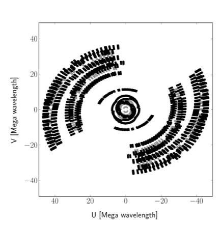
Figure 1: Example of the UV-coverage of the phase-calibrator source J1722+5856, observed 29th October 2005 (date A). Gray points display the UV coverage lost by excluding the WSRT array. The radial extend of the individual scans are due to the large frequency coverage of 128 MHz.

calibrator		amplitude on individual run [mJy]		mean $\pm$ rms [mJy]	calibrated with
	A	B	C
J1722$+$5856	136.90 $\pm$ 2.14	141.48 $\pm$ 0.81	130.76 $\pm$ 1.91	136.38 $\pm$ 5.37	J1722$+$5856
J1722$+$6105	174.70 $\pm$ 9.13	152.91 $\pm$ 21.9	174.31 $\pm$ 34.7	167.31 $\pm$ 12.5	J1722$+$5856
J1722$+$6105	167.02 $\pm$ 5.33	160.27 $\pm$ 1.40	170.38 $\pm$ 3.50	165.89 $\pm$ 5.15	J1722$+$6105

Table 1: Calibrator flux densities. J1722+5856 was used as a phase reference source for all the three observation runs. Source 1722+6105 was used to test the phase-referencing technique and quantify uncertainties in amplitude. Using J1722+6105 calibrated with J1722+5856, an estimate of the night-to-night variation in amplitude is obtained, with an uncertainty of 7% (167.31$\pm$12.5). Comparing the amplitudes of J1722+6105 calibrated using J1722+5856 and with itself, the uncertainty in amplitude due to phase referencing is estimated to be 5% on any individual run (e.g. compare 152.91 and 160.27 on date B). Adding these in quadrature the total amplitude uncertainty is therefore estimated to be 9%.

source	z	optical	radio	peak flux density [mJy]	rms [mJy]	significance [sigma]	$\Delta$ra [mas]	$\Delta$dec [mas]
AMS01B	2	B	SSS	165.03	33.67	4.9	-672	-203
AMS03B	2.698	NL	SSS	1118.00	45.24	24.7	98	35
AMS05B	2.850	NL	GPS	856.30	36.72	23.3	-7	-181
AMS06B	1.8	B	SSS	147.79	31.23	4.7	1327	881
AMS09C	2.1	B	SSS	249.3	32.6	7.6	-185	36
AMS12A	2.767	NL	SSS	222.1	41.5	5.4	-70	-123
AMS15A	2.1	B	FSS	198.6	28.2	7.0	213	140
AMS16A	4.169	NL	GPS	163.9	29.3	5.6	-55	1432
AMS17A	3.137	NL	SSS	151.3	29.3	5.2	967	-843
AMS19C	2.3	B	FSS	599.4	38.1	15.7	10	34
AMS21C	1.8	B	SSS	221.7	30.0	7.4	90	86

Table 2: The target source names are labelled with the observing dates A, B, or C. It was not possible to optain spectroscopic redshift for AMS01, so a fiducial value of 2 is assumed. For all other sources spectroscopic redshifts are quoted. Redshifts with three decimal are from optical spectroscopy, while those with one decimal place are from mid-infrared spectroscopy (MS06a; MS08). The redshift for AMS05 comes from Smith et al. (2009). The third column summarizes the optical spectroscopic properties: B stands for blank spectrum, NL for narrow lines. The fourth column summarizes the low resolution radio spectral indices: FSS stands for flat-spectrum source, GPS for gigahertz-peaked source, and SSS stands for steep-spectrum source. Target peak flux densities per beam. Amplitude measurements of the individual target sources are based on the dirty images. The offsets $\Delta$ra and $\Delta$dec are with respect to the B-array (1.4 GHz) VLA positions of Condon et al. (2003).

Name	Datea	RAb	Dec	$S_{peak}$c	$S_{int}$c	$\theta_{M}$x$\theta_{m}$d	Distancee	$\alpha^{1.4}_{0.6}$f	$\alpha^{4.9}_{1.4}$f
		[J2000]	[J2000]	[$\mu$Jy/beam]	[$\mu$Jy]	[mas2]	[deg]
AMS01	$B$			$<$139.2 / 27.9	$<$136.2 / 47.6		1.242	1.0$\pm$0.2	0.9$\pm$0.6
AMS03	$B$	17 13 40.2037	+59 27 45.795	1139.4$\pm$44.6	1238.3$\pm$81.6	18x13	1.251	1.2$\pm$0.2	1.4$\pm$0.3
AMS05	$B$	17 13 42.7650	+59 39 20.039	923.3$\pm$46.6	992.9$\pm$84.8	18x14	1.333	0.2$\pm$0.2	0.7$\pm$0.2
AMS06	$B$			$<$128.7 / 25.5	$<$125.3 / 43.3		1.227	1.1$\pm$0.2	0.7$\pm$0.5
AMS09	$C$	17 14 34.8448	+58 56 46.467	233.9$\pm$33.0	326.9$\pm$71.8	24x16	1.036	1.2$\pm$0.2	0.7$\pm$0.5
AMS12	$A$	17 18 22.6407	+59 01 54.135	210.2$\pm$27.1	240.7$\pm$51.3	19x14	0.552	1.2$\pm$0.2	0.9$\pm$0.5
AMS15	$A$	17 18 56.9549	+59 03 25.091	201.7$\pm$24.5	202.4$\pm$42.5	25x23	0.485	0.3$\pm$0.2	0.2$\pm$0.3
AMS16	$A$			$<$158.8 / 20.3	$<$210.5 / 42.5		0.407	$<$-1.0	$>$1.02
AMS17	$A$			$<$154.1 / 22.5	$<$139.4 / 36.5		0.499	1.0$\pm$0.2	0.7$\pm$0.4
AMS19	$C$	17 20 48.0000	+59 43 20.687	642.8$\pm$69.9	789.5$\pm$139.	21x16	0.816	0.2$\pm$0.1	0.4$\pm$0.2
AMS21	$C$	17 21 20.0974	+59 03 48.644	231.8$\pm$30.5	258.6$\pm$56.8	18x14	0.206	1.0$\pm$0.2	0.9$\pm$0.7

Table 3: Radio properties of obscured radio intermediate quasars observed with the EVN. Each source has been observed for $\sim$1 hour with a bandwidth of 128 MHz at a central frequency of 1658.24 MHz. ^aDates $A$ and $B$ correspond to the 29 and 30 October 2005, respectively, and date $C$ to the 1st November 2005. ^bThe estimated positions of the EVN radio emission. Comparing the EVN positions with the VLA-B positions at 4.9 GHz the maximum offset is 255 mas. ^cThe peak and integrated flux densities and their errors are based on a Gaussian model fit to individual sources. For consistency the measurements have been determine for all sources in the same manner. For sources with a significance $\geq$6$\sigma$ and AMS12 are provided, whereas for the non-detection the flux densities and errors are given as upper limits. ^d$\theta_{M}$ and $\theta_{m}$ are the mean semi-major and semi-minor axis of the fitted Gaussian, respectively, whereas the array convolved beam is 17$\times$14 mas². ^eThe distance is the radial separation of the observed sources to the phase-reference source J1722+5856. Distances of the undetected sources are based on their VLA-B positions (MS06b). ^fThe spectral indices $\alpha$ and errors between 610 MHz and 1.4 GHz [GMRT, VLA], and between 1.4 and 4.9 GHz are based on the measurements from MS06b [VLA].

EVN observations at 1.66 GHz were performed on the 29th, 30th October and 1st November 2005, hereafter dates $A$, $B$ and $C$. The telescopes used during these observations form an array with baselines ranging of 266 km to 8476 km [Effelsberg, Onsala (85 ft), Jodrell Bank (Lovell), Medicina, Torun, Urumqi, Shanghai and WSRT (phased array)]. The WSRT data on the target sources were lost due to technical problems. This results in an array having a shortest baseline of $\sim$637 km which corresponds to a spatial sensitivity of $\mathrel{\hbox{\hbox to0.0pt{\hbox{\lower 2.0pt\hbox{$\sim$}}\hss}\raise 2.0pt\hbox{$<$}}}$62 mas. Flux which is extended over scales larger than $\sim$62 mas is invisible to the interferometer.

The observations used the Mark5A recording system (1024 Mbit/s) with 2-bit sampling, in 2 polarizations and 2s integration time. The high data rate capability allows the simultaneous observation of 8 sub-bands. Each of the sub-bands has 32 channels with a bandwidth of 16 MHz. Such a large bandwidth could not be handled at the WSRT and the Medicina observatory and therefore one sub-band was lost from these sites. The total frequency coverage is from 1594.99 MHz to 1704.49 MHz which results in a central frequency of 1658.24 MHz. The large fractional bandwidth $\sim$8% significantly increases the UV coverage. As an example, the UV-coverage of the phase calibrator source is shown in Figure 1. With an on-source integration time of $\sim$1 hour, the expected sensitivity in a naturally weighted image is $\sim$20 $\mu$Jy.

Due to the faintness of the actual targets, the observations made use of the phase-reference technique, observing a target and a phase-calibrator source within a cycle of 13 minutes (target source 10 minutes and J1722+5856 for 3 minutes). The target sources are between 0.2 and 1.5 degrees apart from the phase-calibrator source. Additional sources were observed to find initial fringes (J2005+7702, 3C345) and to cross check the phase-referencing technique (J1722+6105, J171156.0+590639).

After observations the data were correlated at the Joint Institute for VLBI in Europe [JIVE]. The positions of the target sources were determined on the basis of VLA-B array observations at 5 arcsec resolution (FWHM). The integration time (2s) and the number of channels assure that the usable field of view (FoV) of the EVN observation is larger than the synthesised VLA beam. Furthermore, this setup ensures that the expected loss in amplitude due to time-smearing will only reach $\sim$10% at a distance of 16.7 arcsec from the pointing centre. Similarly, the loss of amplitude due to bandwidth smearing will only reach $\sim$10% at 9.9 arcsec. An additional effect that could cause a loss in flux density is the variation in the phases caused by the ionosphere. Plotting the fraction of the detected radio emission versus the angular distance to the phase centre does not show any hints of a negative correlation (Fig. 2) and therefore any such flux density losses can probably be neglected.

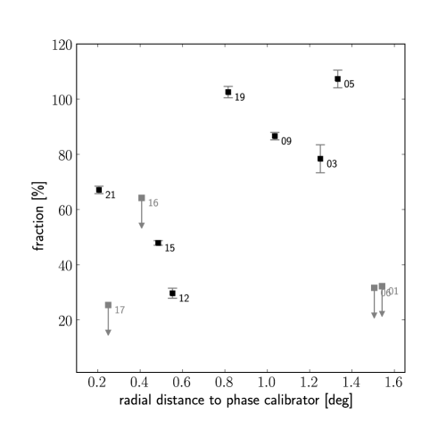
Figure 2: Recovered radio emission in percent versus the radial distance to the phase-calibrator source J1722+5856. The black squares indicate the detected sources. The gray squares and arrows indicate the 6$\sigma$ upper limits of the undetected sources. The median value is 64 %. No significant correlation is found (null hypothesis of no correlation has a probability of 52% and cannot be rejected [using the ASURV software; Isobe, Feigelson & Nelson, 1986; Isobe & Feigelson, 1990]). This supports our contention (see Section 2) that there is no systematic loss in mapped EVN target flux density with separation from the phase calibrator as might be expected if time variations in ionospheric phase were the cause of systematic reductions in the EVN flux density of the sources.

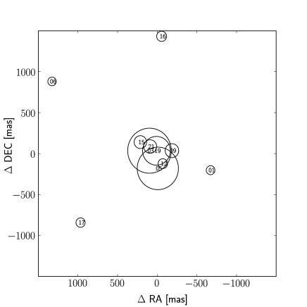
Figure 3: Displacement in ra and dec of the peak flux densities in the dirty images compared with the VLA positions from Condon et al. (2003). The radii of the circles are proportional to the significance of the peak flux density compared to the noise in the dirty map.

Data reduction and analysis were performed using AIPS and ParselTongue (Greisen 1990, ; Kettenis et al. 2006, ). To make sure that all the observing runs were treated in equal manner, a ParselTongue script was developed to calibrate the individual observing runs.

Prior to the calibration the datasets were inspected for bad data. All datasets show narrow band radio interference (RFI) some of which is variable with time. In all the observation runs the RFI was detected in the same channels and sub bands and could be flagged in a similar way using the AIPS task UVFLG. Additional flagging was applied using the flagging tables provided by the VLBI scheduling program SCHED and by the AIPS task QUACK. To account for instrumental polarisation effects a parallactic angle correction has been applied by CLCOR. The observational data were a-priori gain (amplitude) calibrated by using the system temperatures (T_sys) measured at each individual telescope (ANTAB). Prior dispersive delay corrections are applied by the AIPS task TECOR using the ionosphere electron content obtained from the Jet Propulsion Laboratory (see also the explanation file at the TECOR task in AIPS). The sub-band phase offsets have been corrected using the task FRING on the fringe-finding calibrator J2205+7752 for the observations A, B and 3C 345 for C. The residual delays and fringe-rates were then calibrated by initial fringe finding on the phase-reference source J1722+5856 (using the AIPS task FRING; for a full explanation on fringe finding see Cotton 1995).

The bandpass of the system has been calibrated by using the phase-reference-source J1722+5856 (CPASS). After applying the amplitude and phase calibration solution and the bandpass the data show significant offsets in the amplitude over the entire frequency space, whereas the phase stays constant within 1 degree. Such offsets in amplitude can be explained by faulty T_sys measurements caused, e.g. by RFI, which are present at most observatories and individual sub-bands. The amplitude offsets could not be corrected by a full self-calibration procedure on the phase calibrator itself (CALIB). Instead the error has been treated as a baseline based error and the task BLCAL has been used to determine a single solution of the phase and the amplitude for the entire observation. After applying the baseline corrections, amplitude offsets between the individual sub-bands were no longer present.

The final UV-dataset has been produced by applying the calibration correction of J1722+5856 in phase, in amplitude, bandpass, and baseline excluding 4 channels on each edge of each sub-band. Reducing the total bandwidth in frequency to 96 MHz and the theoretical image sensitivity to $\sim$22.5 $\mu$Jy/beam. The final flagging stage of the UV-dataset was based on the average amplitude using the AIPS task VPLOT.

In order to test the reliability of the phase-calibration technique, two test sources (J1722+6105 and J171156.0+590639) were observed and calibrated in an identical manner to the target sources. Furthermore, to determine the error on the amplitude measurements between the different observing runs, the VLBI calibrator J1722+6105 was additionally calibrated by itself, repeating the same steps as J1722+5856 after the sub-band phase offset calibration. The resulting radio flux density of the calibrator J1722+5856 and the reference calibrator J1722+6105 using both methods are shown in Table 1.

The angular separation between the phase-reference source J1722+5856 and J1722+6122 is 2.16 deg. The amplitude of J1722+6105 resulting from both types of calibration (i.e. using J1722+5856 and using J1722+6105 itself) have a largest intraday difference of 5% on night B. This yields an estimate on the maximal uncertainty on the amplitude in using the phase-reference approach in calibrating targets less than 2 deg away from the phase-reference source.

The amplitudes of the phase reference source J1722+5856 shows a night-to-night variation of about 4%. The test phase calibrator J1722+6105, calibrated in a similar way to the targets sources shows during the 3 observing runs an amplitude uncertainty of about 7%. Whereas calibrating the calibrator with itself, it shows a night-to-night variation of about 3%. Combining the estimates of the uncertainties from phase referencing and from night-to-night variation, 5% and 7%, yields an estimate of the total uncertainty in amplitude of $\sim$9%.

After calibration, the position of the phase-calibrator J1722+5856 is consistent with its position in the VLBI catalogue C-VCS1 (Beasley et al. 2002, ). The position of the test phase-calibrator J1722+6105 after applying the solutions of the phase-reference source J1722+5856 is accurate within 3 mas with respect to the C-VCS1 catalogue.

The percentages of the flux densities recovered at EVN resolution (see Section 3) for each target source are shown in Figure 2. There is no evidence of any systematic reduction of the recovered flux density with distance from the phase calibrator, i.e. a negative correlation in Figure 2.

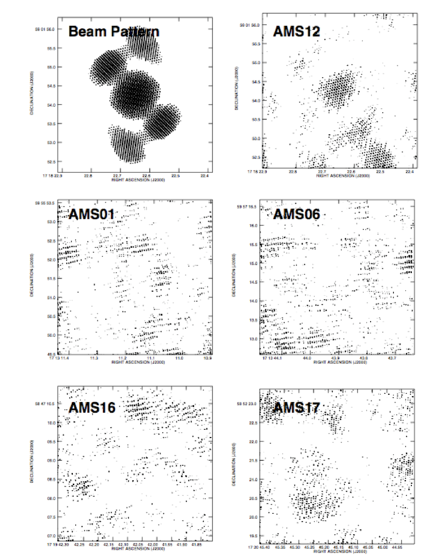
Figure 4: Contour plots covering approximately 4.1$\times$4.1 arcsec² of the beam pattern (for the observations of AMS12) and the dirty images to evaluate detections for sources with peak flux densities below 6$\sigma$. The reference image of the beam has been displayed in the top left corner for which the contours represent 10, 20, 30, and 35% of the maximum. Only positive contours are shown and these peaks and the valleys between these form a grain pattern of characteristic size of the order of the resolution set by the longest baseline. The image shows the characteristic beam and side-lobe levels. For the targets the contours represent 2, 4, 5, 6, 7 $\sigma$, where $\sigma$ is the rms of the image as quoted in Table 1. The source AMS12 shows the characteristic dirty beam and is considered to be a reliable detection.

The imaging procedure was performed in two steps (using the AIPS task IMAGR). First, a dirty image, with robust = 5 (similar to natural) weighting applied, was produced. The field-of-view (FoV) of these dirty images is approximately 4.1$\times$4.1 arcsec², covering practically the entire synthesised beam of the low-resolution VLA images.

For each image, the noise and the highest peak flux density have been determined. For each source these values are shown in Table 2 and the significance of the peak flux densities is represented in Figure 3. Five sources show peak flux densities below 6 $\sigma$ and are shown in Figure 4. Of these sources, 4 are displaced more than 500 mas from the VLA positions (which corresponds to the uncertainty in the Condon et al. 2003 VLA B-array positions at 1.4 GHz).

An example of the synthesized beam pattern is shown in Figure 4. Due to the imaging weighting scheme, the beam pattern produces a large noise floor effecting the determination of the noise. Real detected point sources should show the same beam pattern, although it might be slightly displaced from the VLA positions (the centre of each image). Visual inspection of Figure 4 suggests AMS12 is a safe detection while AMS01 and AMS06 are non-detections. AMS16 and AMS17 show some flux above 5$\sigma$, displaced from the VLA positions. From the images, the significance of the peak flux, and the displacement, these two sources are not considered safe detections. Therefore 6$\sigma$ limits are quoted for the non-detections.

For the sources with peak flux densities above 6$\sigma$ and the secure 5.4$\sigma$ detection (AMS12) cleaned images were produced and are shown in Figure 5. For these final images, the tangent-point of the data was shifted to the centre of the detected emission. The images were produced using a robust weighting of 5 and the central region was cleaned. The properties of the radio emission have been determined using the task IMFIT.

In addition, on the 1st of November the source J171156.0+590639 was also observed in order to test the observing strategy. This source is located 1.38 deg away from the phase-reference calibrator and had already been observed with NRAO’s Very Large Baseline Array (VLBA) at 1.4 GHz. The flux density at 1.4 GHz from the VLBA of 17.03$\pm$1.29 mJy (Wrobel et al. 2004) are, within the errors, consistent with the EVN measurements at 1658.24 MHz of 14.9$\pm$4.4 mJy (32$\times$13 mas²) as shown in Figure 5. The small difference in flux densities is insignificant, and could be explained by the slightly different observed frequencies provided that, at VLBI resolution, J171156.0+590639 has a spectral index $\alpha\sim 0.5$. The source at EVN resolution is slightly elongated in the North-South direction which is consistent with the VLBA observations of Wrobel et al. (2004).

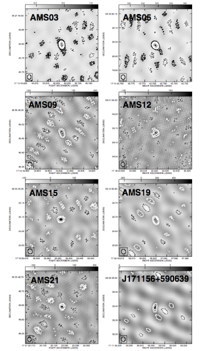
Figure 5: EVN cleaned images covering approximately 260$\times$260 mas² of the radio emission (Stokes I) at 1658.24 MHz  of the 7 securely detected high-redshift obscured quasars. The boxed ellipses show the Gaussian restoring beam at FWHM. The contours are at 30 $\mu$Jy $\times$ 2${}^{\frac{n}{2}}$ (n =-2, 2, 3, etc.). The image at the bottom right displays the radio emission of the comparison source J171156.0+590639 (Wrobel et al. 2004) with contours of 1.78 mJy $\times$ 2${}^{\frac{n}{2}}$ (n =-2, 2, 3, etc.). All these images have been calibrated following the procedure described in Section 2.

3 Results

The EVN observations result in 7 detections and 4 non-detections (AMS01, AMS06, AMS16, and AMS17). Images for the detections are shown in Figure 5. Within the FoV mapped around each source (4.1$\times$4.1 arcsec²) no further radio emission has been detected in any case.

Amongst the detected sources, the integrated fluxes are not significantly higher than the peak fluxes (see Table 3), suggesting the recovered flux originates from an essentially point-like region. The lack of other detections within the field of view around each source rules out the detection of any double cores or knots separated by more than $\sim$150 pc.

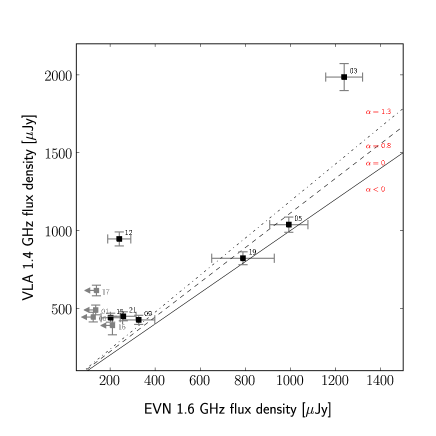
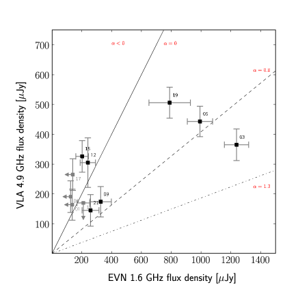
Figure 6: Radio flux densities at 1.4 GHz and 4.9 GHz (VLA-B and VLA-C; MS06b) versus the EVN flux densities at 1658.24 MHz. The solid line displays the track due to a completely flat spectral index ($\alpha=$0.0), the dashed line displays a spectral index of 0.8 and the dashed-doted one of 1.3. The flat spectral indices indicate optically-thick emission, most likely due to an AGN core given the $T_{\rm B}$ inferred. Extended emission from the lobes of jets and emission from star-formation typically lead to optically-thin emission with spectral index around $\alpha=$0.8 (e.g. Condon 1992). Inverse-Compton scattering against the Cosmic Microwave Background can lead to ultra-steep sources with $\alpha\sim 1.3$ (e.g. Kardashev 1962; Röttgering et al. 1994).

In Figure 6, EVN and VLA flux densities are displayed. In the top panel of Figure 6, the clustering of sources around low flux densities is a natural consequence of the 1.4 GHz flux limit used to select the sample. In the bottom panel, less clustering is visible, due to the range of different spectral indices in the sample (see MS06b).

The flux densities at 4.9 GHz at the VLA resolution can be compared to the EVN flux densities at 1.66 GHz, under the assumption that the 4.9 GHz flux emerges from the same physical region as the EVN cores ($\mathrel{\hbox{\hbox to0.0pt{\hbox{\lower 2.0pt\hbox{$\sim$}}\hss}\raise 2.0pt\hbox{$<$}}}$150 pc). Given that the observed 4.9 GHz corresponds to rest-frame between 14 and 25 GHz, this assumption is likely to be appropriate (see e.g. Ulvestad et al. 1999). Under this assumption, spectral indices have been determined for the cores (see Table 4). From Figure 6 and Table 4, six sources show more flux at 4.9 GHz compared to 1.66 GHz, indicating an inverted core spectral index ($\alpha<0$). The remaining sources show less flux at 4.9 GHz than at 1.66 GHz.

Using the spectral index $\alpha^{4.9}_{1.4}$ of Table 3, flux densities at VLA resolution at the frequency of 1.66 GHz have been derived ($S_{\rm VLA1.6}$), to estimate the fraction of the total flux density recovered at EVN resolution. These quantities are shown in Table 4. For the detected sources, the EVN recovers between 29% and 107% of the low resolution flux densities, and the median recovered fraction is 78%. The median fraction including non-detections is 64%, so that typically two thirds of the 1.66 GHz radio flux density is confined to a region of $\mathrel{\hbox{\hbox to0.0pt{\hbox{\lower 2.0pt\hbox{$\sim$}}\hss}\raise 2.0pt\hbox{$<$}}}$150 pc. The percentages for the non-detected sources are $\mathrel{\hbox{\hbox to0.0pt{\hbox{\lower 2.0pt\hbox{$\sim$}}\hss}\raise 2.0pt\hbox{$<$}}}$64% (although mostly $\mathrel{\hbox{\hbox to0.0pt{\hbox{\lower 2.0pt\hbox{$\sim$}}\hss}\raise 2.0pt\hbox{$<$}}}$32%) and for these sources, a compact source with a fraction that is similar to that of some detections (e.g. AMS12), cannot be ruled out.

Table 2 also summarises the optical and low-resolution radio properties of the sources. The recovered fraction for blank-spectrum and narrow-line sources are statistically indistinguishable: the probability of the two samples being drawn from the same underlying distribution is 92% using several two-sample univariate tests (ASURV: Feigelson & Nelson 1985). There is also no correlation between the spectral indices $\alpha^{1.4}_{0.610}$, $\alpha^{4.9}_{1.4}$ and the percentage of the recovered flux. The recovered fraction is apparently independent of the low-resolution radio spectral properties. The characteristics of the detected and the missing flux are discussed in Section 4.

The luminosity densities $L_{\nu}$ at the resolution of the EVN have been calculated using:

$$L_{\nu_{\rm rest}}={d_{\rm lum}^{2}S_{\nu_{obs}}\over(1+z)},$$ (1)

where $\nu_{\rm obs}$ is the observed frequency (1.66 GHz) and $\nu_{\rm rest}=\nu_{\rm obs}\times(1+z)$ is the rest frame frequency, which varies between objects in the sample due to their different redshifts. $S_{\nu}$ is the flux density at 1.66 GHz and at EVN resolution while $d_{\rm lum}$ is the luminosity distance. Since at observed frequencies below 1.66 GHz the spectral indices are not known at mas resolution, the conversion to rest-frame luminosity 1.66 GHz is not possible and no “K-correction” is attempted.

Instead, the luminosities quoted in Table 4, $L_{\nu_{\rm rest}}$, are at $\nu_{\rm rest}=1.66\times(1+z_{\rm spec})$ GHz, where the $z_{\rm spec}$ is the spectroscopic redshift for each source.

The brightness temperature $T_{\rm B}$ has been calculated using:

$$T_{\rm B}=\frac{8\,{\rm log}(2)}{3\pi}\frac{c^{2}}{2\,k}\frac{S_{{\nu}_{obs}}\,(1+z)}{\theta_{M}\theta_{m}},$$ (2)

where $c$ is the speed of light, $k$ is Boltzman’s constant, $\theta_{M}$ and $\theta_{m}$ are the semi-major and semi-minor angular sizes, respectively (Condon et al. 1991). Given that for the detected sources, the median redshift is $z=2.5$, this corresponds to $\nu_{\rm rest}\sim 5.8$ GHz (and to 8.6 GHz in the case of AMS16). The median surface brightness temperature, $T_{B}$, is found to be $10^{6}$ K.

The detected and the missed emission have both been converted to a star-formation rate (SFR), following Condon (1992). The SFRs derived if the missing flux were due entirely to star formation are shown in Table 4. This is discussed further in Section 4.

Name	$z$a	log10($L_{\nu_{\rm rest}}$b	log10($T_{\rm B}$b	$S_{\rm VLA~{}1.6}$c	Fractiond	log10($L_{\nu_{\rm miss}}$e	SFRmissf	$\alpha^{4.9}_{1.6}$$\,{}^{g}$	Diameterh
		[W Hz-1 sr-1])	[K])	[$\mu$Jy]	[%]	[W Hz-1 sr-1])	[M⊙yr-1]	(core)	[pc]
AMS01	2	$<$23.0	–	422	$<$32	$>$23.3	$>$1424	$\leq$-0.17 $\pm$ 1.00	–
AMS03	2.698	24.2	6.8	1579	78 $\pm$ 5	23.6	3249	1.13 $\pm$ 0.34	142
AMS05	2.850	24.1	6.7	925	107 $\pm$ 3	–	–	0.74 $\pm$ 0.30	140
AMS06	1.8	$<$22.9	–	396	$<$31	$>$23.2	$>$1066	$\leq$-0.39 $\pm$ 0.94	–
AMS09	2.1	23.4	5.9	377	86 $\pm$ 1	22.6	279	0.58 $\pm$ 0.78	199
AMS12	2.767	23.5	6.0	811	29 $\pm$ 1	23.9	5737	-0.22 $\pm$ 0.73	149
AMS15	2.1	23.2	5.5	422	47 $\pm$ 0	23.3	1218	-0.44 $\pm$ 0.56	208
AMS16	4.169	$<$23.7	6.0	$\leq$327	$<$64	$>$23.5	$>$2764	$\sim$0.62	–
AMS17	3.137	$<$23.4	5.8	548	$<$25	$>$23.8	$>$5363	$\leq$-0.59 $\pm$ 0.70	–
AMS19	2.3	23.9	6.4	769	102 $\pm$ 2	–	–	0.41 $\pm$ 0.43	172
AMS21	1.8	23.2	5.9	385	67 $\pm$ 1	22.9	499	0.53 $\pm$ 0.91	152

Table 4: Properties of the obscured quasars. ^aRedshifts, are all spectroscopic except for AMS01. Redshifts with three decimal are from optical spectroscopy, while those with one decimal place are from mid-infrared spectroscopy (MS06a; MS08). The redshift for AMS05 is from Smith et al. (2009). ^bMonochromatic EVN luminosity and brightness temperatures at restframe frequency $\nu_{\rm rest}=\nu_{\rm obs}\times(1+z)$. Note that the spectral index at small scales is not known and therefore no K-correction has been applied: both the the luminosity densities and the brightness temperatures are calculated in the rest frame using Eq. 2. ^cExpected total flux density (i.e. at VLA resolution) at the EVN observing frequency of 1.66 GHz. This was estimated using radio spectral indicees based on the VLA measurements by MS06b. ^dEstimated fraction of total flux density at 1.66 GHz recovered at the resolution of the EVN, the quoted uncertainties do not include the 9% uncertainty on the amplitude inferred from the phase callibrators. ^eLogarithm of the monochromatic restframe luminosity of the non-detected (missing) radio emission, calculated with Eq. 1. The star-formation rate of the undetected radio emission. ^fThis star-formation rate is calculated for massive stars only ($M_{\star}\geq 5$ M_⊙). ^gCore spectral index assuming that all the VLA emission emerges from the same physical region as the EVN emission. ^hUpper limits on the physical extend of the EVN emission region. The maximum of the deconvolved beam size is $\sim$17 mas, which translate at the median redshift of 2.3 to a physical extend of 137 pc (approx. 150 pc).

4 Discussion

Most of the observed sources show compact radio emission at physical sizes $\mathrel{\hbox{\hbox to0.0pt{\hbox{\lower 2.0pt\hbox{$\sim$}}\hss}\raise 2.0pt\hbox{$<$}}}$150 pc, and this emission accounts for a significant fraction ( $\mathrel{\hbox{\hbox to0.0pt{\hbox{\lower 2.0pt\hbox{$\sim$}}\hss}\raise 2.0pt\hbox{$<$}}}$30% up to $\sim$100%) of the total radio emission. In the following discussion, the flux density detected by the EVN observations is referred to as the “core”. For the missing flux, resolved out by the EVN, there is no information about the structure or extent. This radio emission could, in principle, emerge from star-formation on either circum-nuclear or galactic scales, from the radio emission due to a jet, or a combination of both. The two limiting cases are considered here.

4.1 The detected radio emission

For the core emission in detected sources, the median brightness temperature, $T_{B}=10^{6}$ K (see Table 4), is slightly high compared to synchrotron radiation from supernovae (SNe) and SNe remnants only. The regions with radio emission due to star-forming typically have $T_{\rm B}\mathrel{\hbox{\hbox to0.0pt{\hbox{\lower 2.0pt\hbox{$\sim$}}\hss}\raise 2.0pt\hbox{$<$}}}10^{5}$ K (Muxlow et al. 1994, ), however the values of $T_{B}$ in this sample are close to the limiting value. Therefore, the possibility that the radio emission detected by the EVN are in fact dense star-forming regions needs to be considered.

The detected cores have a median luminosity, $L_{\rm rest}=3\times 10^{23}$ W Hz^-1 sr^-1. If this emision was due to star-formation only, then the estimated star-formation rate (SFR), following Condon (1992), would correspond to a SFR $\sim 3600$ M_⊙ yr^-1 (of massive stars only $\geq 5$ M_⊙), and integrating over a Salpeter (1955) initial mass function (IMF) would result in a median total SFR of $\sim 14~{}000$ M_⊙ yr^-1. The extremely high SFRs derived in this way, and quoted in Table 4, are comparable or generally greater than the SFRs inferred for submillimetre-selected galaxies (Smail et al. 1997, ), except here they are confined to a significantly smaller volume. Given that the resolution of 17 mas corresponds to typically 150 pc  at $z=2.3$, these cores have physical sizes comparable to those of the “extreme starburst” regions found by Downes & Solomon (1998), but the SFRs are about two orders of magnitude higher. These are unreasonable SFRs for such a small region.

The hypothesis of the detected cores being dense star-formation regions can also be rejected on the basis of the mass of molecular gas required to power such a SFR. An estimate of the typical star-formation density of the cores, assuming a total SFR of 14 000 M_⊙ yr^-1  in an area with diameter a 200 pc corresponds to $\Sigma_{\rm SFR}$$=1.1\times 10^{5}$ M_⊙ yr^-1  kpc^-2. Thus, if these cores followed the Kennicutt-Schmidt law [${\Sigma_{SFR}}=$${2.5\times 10^{-4}}$${{({{\Sigma_{gas}}\over{1~{}M_{\odot}~{}{\rm pc}^{-2}}})}^{1.4}}$ M_⊙ yr^-1 kpc^-2, Kennicutt 1998], they would have extreme gas densities of $\Sigma_{\rm gas}=$$1.5\times 10^{6}$ M_⊙ pc^-2, or a gas mass of $1.9\times 10^{11}$ M_⊙ (in a characteristic size $\mathrel{\hbox{\hbox to0.0pt{\hbox{\lower 2.0pt\hbox{$\sim$}}\hss}\raise 2.0pt\hbox{$<$}}}$150 pc). Such extreme molecular gas masses have been observed around high-redshift quasars, but they are extended over $\sim$kpc scales and not in such a small nuclear region (e.g. Walter et al. 2004). Thus, the hypothesis that the detected cores are dominated by star-formation can be safely rejected, and in the rest of this section we assume the cores to be due to an AGN.

Table 4 quotes the core spectral indices, $\alpha^{4.9}_{1.6}$, derived assuming that all the flux density at 4.9 GHz at VLA resolution emerges from a region comparable to the EVN resolution. Overall the spectral indices appear to be either relatively steep, or inverted. However, we note that within the uncertainties, most of the inverted spectra could be flat.

The flat or inverted spectrum can be understood as synchrotron self-absorption due to a high density of relativistic electrons causing the emission to be optically thick. However, none of the spectral indices are close to the expected value of $\alpha=-2.5$ for an entirely self-absorbed regime (Rybicki and Lightman 1979). Such observed flat spectra can be observed if the transition between optically-thin and optically-thick (and therefore the peak in the spectrum) occurs at a frequency somewhere between 5.8 and 17 GHz. The expected spectral indices would then be relatively flat, consistent with those seen in Table 4. Alternatively, several emitting components, each of which becomes self-absorbed at a different frequency, when superimposed, can lead to the observed spectral indices.

It is worth noting that the sources with high recovered fractions (that is AMS03, AMS05, AMS09 and AMS19) have core spectral indices indistinguishable from the low-resolution spectral indices. This suggests the physical source of the EVN flux is also the dominant component of the emission detected by the VLA and therefore apparently compact. The actual mechanisms, however, probably vary from source to source, as described below.

In the case of AMS05 and AMS16, the total (low-resolution) spectra appear gigahertz-peaked (MS06b), reminiscent of the young compact powerful radio sources (O’Dea 1998). The core spectral index of AMS05 is consistent with the low-spatial resolution spectral index (between VLA observations at 1.4 and 4.9 GHz), and 100% of the low-resolution flux density is recovered. This suggests the same emission is being seen at VLA and EVN resolutions, so that the dominant source of radio emission is compact ($\mathrel{\hbox{\hbox to0.0pt{\hbox{\lower 2.0pt\hbox{$\sim$}}\hss}\raise 2.0pt\hbox{$<$}}}$150 pc). This also agrees with the hypothesis of synchrotron self-absorption affecting frequencies around and below 5–6 GHz, while the emission at frequencies higher than this is still optically-thin and therefore shows a steep spectrum. The core spectral index of AMS16 is ill defined, since the source is not detected at either 4.9 or 1.66 GHz, however a similar argument to that of AMS05 would apply.

Most of the other sources have values of $\alpha^{4.9}_{1.6}$ much flatter than their overall $\alpha^{4.9}_{1.4}$ value at VLA resolution. This is consistent with the following (simplified) scenario: flat spectrum emission from an optically-thick core contributing a significant fraction of the total luminosity, and steep-spectrum emission from optically-thin lobes from a jet. At EVN resolution, the emission from the jet lobes is resolved out, so that the core dominates, and the spectral indices appear flat or inverted.

A slight modification is required in the case of AMS15 and AMS19: their low-resolution spectral indices are also flat. This can be explained by Doppler-boosting of the emission from the core, which would make it a more important contributor to the low-resolution spectrum, which would then appear overall flat. In the case of AMS19, the core spectral index is also flat, and 100% of the flux is recovered, consistent with the beaming scenario. AMS15 has an inverted core spectrum, and the EVN recovers only 47% of the low-spatial resolution flux density.

Doppler-boosting is only expected when the radio jet is closely aligned with the line-of-sight, so the jet must be close to face-on. In the unified scheme, only unobscured quasars can have such a configuration. AMS15 and AMS19 are obscured quasars with a face-on radio jet, and neither show emission lines in their optical spectra. These two objects are probably not obscured by the torus of the unified scheme, but rather by dust on a larger scale, presumably distributed along the host galaxy. This provides further evidence for the hypothesis of “host-obscuration” in some quasars (Martínez-Sansigre et al. 2005; MS06a; Rigby et al. 2006).

At first sight, one might expect flat-spectrum or gigahertz-peaked sources to have the highest detection rates, and that is indeed the case of AMS05 and AMS19. However, some of the sources with the highest recovered fraction (e.g. AMS09 and AMS21) have steep spectra overall. This can be reconciled if the total emission from AMS09 and AMS21 is dominated by radio emission from the lobes of jets, but these jets are small, with an extent limited to a few hundred pc. The high recovered fractions (67 and 86%) are caused by most of the lobe emission being on scales smaller than the beam size, so that only a small fraction of the emission is resolved out. The “core” spectral indices of AMS09 and AMS21 are both $\sim$0.5, but within the large uncertainties they agree with the total spectral indices (at low resolution) between 1.4 and 4.9 GHz (compare their values in Tables 3 and 4). This is in agreement with the suggestion that the “cores” of these two sources are actually unresolved lobes, and indeed the image of AMS09 hints at some extended structure (Figure 5). These sources appear to be lower-luminosity analogues to compact steep-spectrum sources (O’Dea 1998).

4.2 The missing radio emission

In MS06a, the flux densities of this sample at 1.4 GHz obtained by the VLA (5-arcsecond resolution, from Condon et al. 2003) and WSRT (14-arcsecond resolution, from Morganti et al. 2004) were compared and found to be consistent within the errors. There is no evidence for the VLA to ‘resolve out’ flux at 1.4 GHz on scales $\geq 5$ and $\leq 14$ arcseconds, and the the VLA flux densities at 1.4 GHz (and $S_{\rm VLA1.6}$) can be safely considered to represent the entire flux densities of the radio sources at $\sim$GHz frequencies.

There is no intermediate resolution data, and thus no information on scales $\geq 17$ mas and $\leq 5$ arcseconds, and therefore the extent of the missing radio emission correspond to $\mathrel{\hbox{\hbox to0.0pt{\hbox{\lower 2.0pt\hbox{$\sim$}}\hss}\raise 2.0pt\hbox{$>$}}}$150 pc  and $\mathrel{\hbox{\hbox to0.0pt{\hbox{\lower 2.0pt\hbox{$\sim$}}\hss}\raise 2.0pt\hbox{$<$}}}$40 kpc. Again there is the possibility that the radio emission at intermediate size scales is produced by star-formation, or jet activity or a combination of both. Similar arguments for the core are used to discuss the nature of the radio emission:

1. The entirety of the missing flux is due to star-formation. Following Condon (1992), the estimated SFRs are in the range $\sim 500-6000$ M_⊙ yr^-1(see Table 4). This is only for massive stars, with masses $M_{\star}\geq 5$ M_⊙, so the total star-formation rates would be $\sim 4\times$ greater if integrated over a Salpeter IMF. Thus, except in the cases of AMS09 and AMS21 (and maybe AMS15), these are unphysically high SFRs. This is not surprising, since this sample was selected using a radio criterion to avoid contamination by luminous starbursts. Thus, in the sample as a whole, it is extremely unlikely that the missing flux is all due to star-formation.

2. If the missing flux is instead all due to AGN jets, then the median jet luminosity is $L_{\nu_{\rm miss}}=2\times 10^{23}$ W Hz^-1 sr^-1, comparable to RQQ, RIQ, and FR I radio galaxies. Therefore, it is most likely that the missing flux is dominated by emission from jets or lobes on physical scales $\mathrel{\hbox{\hbox to0.0pt{\hbox{\lower 2.0pt\hbox{$\sim$}}\hss}\raise 2.0pt\hbox{$>$}}}$150 pc, and $\mathrel{\hbox{\hbox to0.0pt{\hbox{\lower 2.0pt\hbox{$\sim$}}\hss}\raise 2.0pt\hbox{$<$}}}$40 kpc.

For the sources AMS09, AMS15 and AMS21, the missing flux suggest reasonable SFRs, indicating a significant contribution from star-formation cannot be ruled out. However, the cores of all 3 objects are clearly AGN dominated (see Section 4.1). For the rest of the sample, although the extended emission is likely to be completely dominated by AGN emission, it is not possible to rule out the additional presence and thus contribution of a powerful starburst.

4.3 Comparing the core to the total emission

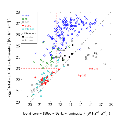
Figure 7: Total luminosity ($\nu_{\rm rest}\sim 1.4$ GHz) versus core luminosity at $\nu_{\rm rest}\sim 5$ GHz. The total luminosity densities of the sample of obscured quasars have been K-corrected with the spectral index $\alpha^{1.4}_{610}$. For the other samples an average spectral index of 0.8 has been assumed. To allow comparison, all the cores luminosity densities have been K-corrected using a spectral index of 0. The diagonal line indicates equality. The horizontal and vertical lines represent the luminosity for a SFR of 1000 M_⊙ yr^-1(all stars of 0.25 to 100 M${}_{\hbox{$\odot$}}$, integrated over a Salpeter IMF), at 1.4 and 5 GHz, respectively. The detected sources from this work are indicated by black rectangles while the grey rectangles and arrows show upper limits of the non-detections. In addition the total and core luminosities are shown for the FR II and FR I sources of the 3CRR catalogue (Blundell et al. in prep.), a sub-sample of the Bright Quasar survey (BQS, Miller et al. 1992; 1993), Ultra-luminous infrared galaxies (ULIRG, Smith et al. 1998, ) and a sample of radio-quiet quasars (Kukula et al. 1998).

Based on the discussion in Sections 4.1 and 4.2, both the core and most of the missing radio emission are dominated by AGN emission. The extended emission is unconstrained within the range $\mathrel{\hbox{\hbox to0.0pt{\hbox{\lower 2.0pt\hbox{$\sim$}}\hss}\raise 2.0pt\hbox{$>$}}}$150 pc  and $\mathrel{\hbox{\hbox to0.0pt{\hbox{\lower 2.0pt\hbox{$\sim$}}\hss}\raise 2.0pt\hbox{$<$}}}$40 kpc. It is therefore both interesting and meaningful to compare the radio properties of this sample to those of other samples of AGN, particularly given that the total luminosities of the sources are comparable with those of RIQ and FR I, and the core luminosities of the observed sources are also similar to the core luminosities of local FR I, which range between 10²² –10²⁴ W Hz^-1 sr^-1  (e.g. Zirbel & Baum 1995, ).

Figure 7 shows the total luminosity density versus core luminosity density for other samples of AGN: FR I and FR II sources from the 3CRR sources (Blundell et al. in prep.), a sub-sample of the Bright Quasar survey (BQS, Miller et al. 1992; 1993), ULIRGs (Smith et al. 1998, ) and a sample of radio-quiet quasars (Kukula et al. 1998, actually a subsample of the Miller et al. 1993 sample).

The obscured quasars observed in this paper show a narrow distribution of the ratio of their total to core luminosities, i.e. these luminosities being correlated, with the null hypothesis having a probability 0.02% (ASURV software using the sub-routine BIVAR). The total luminosities are therefore related by a linear regression with log($L_{\rm tot}$) $\sim$ (3.5$\pm$1.9) log($L_{\rm core}$). The sample of RQQ shows a correlation significant at the $\geq 3\sigma$ level with log($L_{\rm tot}$) $\sim$ (1.0$\pm$0.1) log($L_{\rm core}$), the FR I sources show a slope of 0.7$\pm$0.2 (97% confidence) while the FR II sources have 0.4$\pm$0.1 ($\geq 3\sigma$ significance). Hence, as well as having similar recovered fractions to the RQQ, there are hints that the obscured quasars show a slope more similar to the RQQ than the FR I or FR II sources. Overall, the obscured quasars appear more similar to the RQQ than any of the FR I or FR II radio sources, although the errors in the small sample of objects observed in this paper are high.

The observations are at a range of different frequencies, which have been converted to approximately 5 GHz (rest-frame). The luminosities of obscured quasars are at $\nu_{\rm rest}=\nu_{\rm obs}\times(1+z)$, corresponding to around 5.8 GHz. This small difference is not important: the main result of Figure 7 is that the sample of obscured quasars shows similar core-to-total luminosity ratios to the radio-quiet and radio-intermediate quasars (as well as, for example, to Mrk 231; Ulvestad et al. 1999; Klöckner et al. 2003). In these samples, the core emission reprents a large fraction of the total emission, whereas in FR I and FR II sources, the total emission is typically $\geq$1 dex greater than the core emission.

In the sample of obscured quasars, typically $\sim$60% of the flux is recovered on scales $\mathrel{\hbox{\hbox to0.0pt{\hbox{\lower 2.0pt\hbox{$\sim$}}\hss}\raise 2.0pt\hbox{$<$}}}$150 pc, and both flat-spectrum or inverted cores are inferred. The distributions of recovered fraction from the sample presented here and from the RQQ sample of Kukula et al. (1998) are indistinguishable. For many of the objects the physical scales are only constrained to be $\mathrel{\hbox{\hbox to0.0pt{\hbox{\lower 2.0pt\hbox{$\sim$}}\hss}\raise 2.0pt\hbox{$<$}}}$1 kpc. However, amongst their lowest-redshift sources ($z\sim 0.05$) the VLA-A array resolution at 8.4 GHz is 0.24 arcseconds, which corresponds to $\sim$230 pc scales, and again the distribution of recovered fractions is similar to that of the $z\mathrel{\hbox{\hbox to0.0pt{\hbox{\lower 2.0pt\hbox{$\sim$}}\hss}\raise 2.0pt\hbox{$>$}}}2$ obscured quasars. The main difference is that the typical spectral index inferred for the cores of Kukula et al. is $\sim$0.7. About half of the sample presented here has core spectral indices consistent with those of Kukula et al. (1998), while the other half have inverted (or, given the errors, possibly flat) spectra.

The RQQ and Seyferts show a correlation between $M_{\rm V}$ and $L_{\rm 8.4~{}GHz}$. The obscured quasars have mid-infrared luminosities that correspond to unobscured quasars with estimated values of $-26\mathrel{\hbox{\hbox to0.0pt{\hbox{\lower 2.0pt\hbox{$\sim$}}\hss}\raise 2.0pt\hbox{$<$}}}M_{\rm B}\mathrel{\hbox{\hbox to0.0pt{\hbox{\lower 2.0pt\hbox{$\sim$}}\hss}\raise 2.0pt\hbox{$<$}}}-24$ (see MS06a and Smith et al. 2009), and radio luminosities at $\sim$6 GHz of $10^{23}-10^{24}$ W Hz^-1 sr^-1. Assuming $M_{\rm B}\approx M_{\rm V}$ and $L_{\rm 8.4~{}GHz}\approx L_{\rm 6~{}GHz}$, for a given value of $M_{\rm V}$, the obscured quasars are $\sim$2 dex more powerful in radio luminosity compared to the RQQs. This fits in with the results of Figure 7: the high-redshift obscured quasars have compact-to-total ratios similar to those of RQQ, and extended emission on comparable scales, yet the RQQ are significantly less powerful at radio frequencies.

Finally, given that the obscured quasars have radio luminosities corresponding to RIQ, and that $\sim$40% of the flux density is in an extended component, it is clear that the majority of them are not beamed, and that their luminosity densities are intrinsic.

5 Conclusions and summary

A subsample of 11 high-redshift obscured quasars has been observed at 1.66 GHz with the EVN, reaching a noise level of $\sim$ ${\rm 25~{}\mu Jy~{}per~{}17\times 14~{}mas^{2}~{}beam}$. The observations are sensitive to radio emission on physical scales $\mathrel{\hbox{\hbox to0.0pt{\hbox{\lower 2.0pt\hbox{$\sim$}}\hss}\raise 2.0pt\hbox{$<$}}}$150 pc. Seven sources are securely detected and show compact radio emission.

Amongst the detections, $\sim$30–100% of the entire flux density is recovered in the core. Considering the luminosity densities and brightness temperatures, and comparing them to SNe brightness temperatures as well as SFRs and molecular gas masses of extreme starbursts, the cores are found to be AGN-dominated and not due to a nuclear starburst. In the non-detections, the limits inferred for the radio emission and inferred properties are similar to those of the detected cores.

Comparing the total and core flux densities and spectral indices, the sample is found to contain a mixture of steep-spectrum, gigahertz-peaked spectrum, compact steep spectrum and beamed sources.

When considering the EVN observations, no correlations are found between the optical spectra and the recovered fraction. Hence, there is no difference in the recovered fraction between host-obscured or torus-obscured quasars. Indeed, no correlation is found either between the low-resolution spectral indices and the recovered fraction. This can be explained by the sample being composed of a mixture of steep-spectrum, compact-steep-spectrum, gigahertz-peaked and flat-spectrum sources. Hence, the recovered fraction is related to the size and orientation of the jet rather than the distribution of the obscuring dust.

However, when considering the total (low-resolution) spectral indices and the core spectral indices, two sources are consistent with overall flat spectra due to a Doppler-boosted radio core (from a face-on jet, AMS15 and AMS19). In the unified scheme, only unobscured quasars are expected to show such flat spectra, but neither source shows either broad or narrow emission lines, despite being at redshifts where the rest-frame ultraviolet lines are observable. These two sources are candidates for “host-obscured” quasars, where the obscuring dust is distributed on $\sim$kpc scales, rather than in the torus of the unified scheme.

At the redshifts of the sources, the missing flux densities (the emission ‘resolved-out’ by the EVN) correspond to too high radio luminosities to be consistent with star-formation only in all but a few cases. The extended emission is therefore also interpreted as being dominated by radio emission from the lobes of jets, comparable in luminosity to those of RIQ and FR I radio sources. However, a hybrid scenario with significant on-going star-formation cannot be ruled out.

Since the core and the extended emission are both AGN-dominated, the core and total luminosities of the sources are compared to those of other samples of AGN: RQQ, RIQ, RLQ, FR I and FR IIs. In particular, the total radio luminosities of the obscured quasars are comparable to those of FR I and RIQ. The core-to-total luminosity ratios ($\sim$0.5) are found to be more similar to those of RQQ, rather than FR I sources. Indeed, the RQQ studied by Kukula et al. (1998) had a mean core-to-total luminosity fraction of 0.6 at 4.8 GHz. Although, the cores of their RQQ had typically steep spectral indices, whereas the high-redshift obscured quasars sometimes have inverted or flat cores. However, it is worth noticing that it is very difficult to assess the precise differences between RQQ and FR Is when they have been observed with different interferometers and at different redshifts; inverse-compton scattering against the CMB could extinguish old extended radio jets on larger scales in high redshift objects (e.g. Blundell and Rawlings 2001).

The sample of obscured quasars have higher values of $L_{\rm radio}$ for an estimated $M_{\rm V}$, situating them in the RIQ regime rather than the RQQ. Yet, their properties are more similar to those of RQQ than to FR I sources. These obscured RIQ have overall (low-spatial resolution) steep spectra, and $\sim$40% of the flux is resolved out on $\mathrel{\hbox{\hbox to0.0pt{\hbox{\lower 2.0pt\hbox{$\sim$}}\hss}\raise 2.0pt\hbox{$>$}}}$150 pc  scales, so that they are not all beamed RQQ: they have intrinsically higher luminosities. The sources in our sample therefore reflect a gradual transition of intrinsic luminosities between the values observed for RLQ and for RQQ.

References

- (1) Beasley A.J., Gordon D., Peck A.B., Petrov L., MacMillan D.S., Fomalont E.B., Ma C. 2002, ApJSup., 141, 13
- (2) Blandford R.D., Payne D.G., 1982, MNRAS, 199, 883
- (3) Blandford R.D., Znajek R.L., 1977, MNRAS, 179, 433
- (4) Blundell K.M., Beasley A.J., 1998, MNRAS, 299, 165
- (5) Blundell K.M., Rawlings S., 2001, ApJ, 562, L5
- (6) Blundell K.M., Beasley A.J., Bicknell G.V., 2003, MNRAS, 591, L103
- (7) Cirasuolo M., Magliocchetti M., Celotti A., Danese L., 2003, MNRAS, 346, 447
- (8) Condon J.J., Huang Z.-P., Yin Q.F., Thuan T.X., 1991, ApJ, 378, 65
- (9) Condon J.J., 1992, ARA&A, 30, 575
- (10) Condon J.J., et al., 2003, AJ, 125, 2411
- (11) Cotton W.D., 1995, ASP Conference Series, 82, 189
- (12) Downes D., Solomon P.M., 1998, ApJ, 507, 615
- (13) Falcke H., Sherwood W., Patnaik A.P., 1996, ApJ, 471, 106
- (14) Fanaroff B.L., Riley J.M., 1974, MNRAS, 167P, 31
- (15) Feigelson E.D., Nelson P.I., 1985, ApJ, 293, 192
- (16) Gallimore J.F., Axon, D.J., O’Dea C.P., Baum S.A., Pedlar A., 2006, AJ, 132, 546
- (17) Greisen E., 1990, Acquisition, Processing and Archiving of Astronomical Images, eds. Longo G. and Sedmak G., 125
- (18) Heywood I., Blundell K.M., Rawlings S., 2007, MNRAS, 381, 1093
- (19) Hine R.G., Longair M.S., MNRAS, 1979, 188, 111
- (20) Isobe T., Feigelson E.D., Nelson P.I., 1986, ApJ, 306, 490
- (21) Isobe T., Feigelson E.D., 1990, BAAS, 22, 917
- (22) Ivezić,Ž., et al., 2002, AJ, 124, 2364
- (23) Kardashev N.S., 1962, SvA, 6, 317
- (24) Klöckner H.-R., Baan W.A., Garrett G.A., 2003, Nat, 421, 821
- (25) Krolik J.K, 1999, Active galactic nuclei : from the central black hole to the galactic environment, Princeton University Press
- (26) Kellermann K.I., Sramek R., Schimdt M., Shaffer D.B., Green R., 1989, AJ, 98,1195
- (27) Kukula M.J., Pedlar A., Baum S.A., O’Dea C.P., 1995, MNRAS, 276, 1262
- (28) Kukula M.J., Dunlop J.S., Hughes D.H., Rawlings S., 1998, MNRAS, 297, 366
- (29) Kennicutt R.C., 1998, ApJ, 498, 541
- (30) Kettenis M., van Langevelde H.J., Reynolds C., Cotton B., 2006, ASPC, 351, 497
- (31) Laing R.A., Canvin J.R., Cotton W.D., Bridle A.H., 2006, MNRAS, 368, 48
- (32) Martínez-Sansigre A., Rawlings S., Lacy M., Fadda, D., Jarvis, M. J., Marleau, F. R., Simpson, C., & Willott, C. J., 2005, Nat, 436, 666
- (33) Martínez-Sansigre A., Rawlings S., Lacy M., Fadda, D., Jarvis, M. J., Marleau, F. R., Simpson, C., & Willott, C. J., 2006a, MNRAS, 370, 1479 (MS06a)
- (34) Martínez-Sansigre A., Rawlings S., Garn T., Green, D. A., Alexander, P., Klöckner, H.-R., & Riley, J. M., 2006b, MNRAS, 373, L80 (MS06b)
- (35) Martínez-Sansigre A., Lacy M., Sajina A., Rawlings S., 2008, ApJ, 674, 676 (MS08)
- (36) Miller L., Peacock J.A., Mead A.R.G., 1990, MNRAS, 244, 207
- (37) Miller P., Rawlings S., Saunders R., Eals S., 1992, MNRAS, 254, 93
- (38) Miller P., Rawlings S., Saunders R., 1993, MNRAS, 263, 425
- (39) Morganti R., Garrett M.A., Chapman S., et al., 2004, A&A, 424, 371
- (40) Muxlow T.W.B., Pedlar A., Wilkinson P.N., et al., 1994, MNRAS, 266, 455
- (41) O’Dea C.P., PASP, 110, 493
- (42) Rawlings S., Saunders R., 1991, Nat, 349, 138
- (43) Rigby J.R., Rieke G. H., Donley J. L., Alonso-Herrero A., Pérez-González P. G., 2006, ApJ, 645, 115
- (44) Röttgering H.J.A., Lacy M., Miley G.K. Chambers K.C., Saunders R., 1994, A&AS, 108, 79
- (45) Rowan-Robinson M., 1995, MNRAS, 272, 737
- (46) Rybicki G.B., Lightman A.P, 1979, Radiative Processes in Astrophysics, 190
- (47) Salpeter E.E., 1955, ApJ , 121, 161
- (48) Smith D.J.B, Jarvis M.J., Simpson C., Martínez-Sansigre A., 2009, MNRAS, 393, 309
- (49) Smith H.E., Lonsdale C.J., Lonsdale C.J., 1998, ApJ , 492, 137
- (50) Smail I., Ivison R.J., Blain A.W., 1997, ApJ , 490, L5
- (51) Ulvestad J. S., Wrobel J. M., Carilli C. L., 1999, ApJ, 516, 127
- (52) Urry C.M., Padovani P., 1995, PASP, 107, 803
- (53) Walter F., Carilli C., Bertoldi F., Menten K., Cox P., Lo. K.Y., Fan X., Strauss M.A., 2004, ApJ, 615, L17
- (54) Wrobel J.M., Garrett M.A., Condon J.J., Morganti R. 2004, ApJ, 128, 103
- (55) Williams C.L., Panagia N., Van Dyk S.D., Lacey C.K., Weiler K.W., Sramek R.A., 2002, ApJ, 581, 396
- (56) Zirbel E.L., Baum S. A., 1995, ApJ ,448, 521