Astrophysical constraints on unparticle-inspired models of gravity

Abstract

We use stellar dynamics arguments to constrain the relevant parameters of ungravity inspired models. We show that resulting bounds do constrain the parameters of the theory of unparticles, as far as its energy scale satisfies the condition $\Lambda_{U}\geq 1~{}TeV$ and $d_{U}$ is close to unity.

I Introduction

It has been remarked that the Standard Model (SM) is likely to be incomplete due to the apparent lack of scale invariant objects, unparticles georgi , besides its well-known shortcomings. Implementing scale invariance requires considering an additional set of fields with a nontrivial IR fixed point, the Banks- Zacks (BZ) fields. The interaction between SM and BZ fields occurs through the exchange of particles with a large mass scale, $M_{*}$, written as

$${\cal L}_{BZ}={1\over M_{*}^{k}}O_{SM}O_{BZ}~{}~{},$$ (1)

where $O_{SM}$ is an operator with mass dimension $d_{SM}$ built out of SM fields and $O_{BZ}$ is an operator with mass dimension $d_{BZ}$ built out of BZ fields.

At an energy scale $\Lambda_{U}$ the BZ operators match onto unparticles operators ($O_{U}$) and Eq. (1) matches onto

$${\cal L}_{U}={C_{U}\Lambda_{U}^{d_{BZ}-d_{U}}\over M_{*}^{k}}O_{SM}O_{U}~{}~{},$$ (2)

where $d_{U}$ is the scaling dimension of $O_{U}$, which can be fractional, and $C_{U}$ is a coefficient function.

Considering tensor-type unparticle interactions with the stress-energy tensor of SM states leads to a modification to the Newtonian potential $\Phi(r)$, usually referred to as ungravity — a gravitational potential with a power-law addition ungravity ,

$$V(r)=-{G_{U}M\over r}\left[1+\left({R_{G}\over r}\right)^{2d_{u}-2}\right]~{}~{},$$ (3)

where $R_{G}$ is the characteristic length scale of ungravity,

$$R_{G} = {1\over\pi\Lambda_{U}}\left({M_{Pl}\over M_{*}}\right)^{1/(d_{U}-1)}\times$$

$$\left[{2(2-\alpha)\over\pi}{\Gamma(d_{U}+{1\over 2})\Gamma(d_{U}-{1\over 2})\over\Gamma(2d_{U})}\right]^{1/(2d_{U}-2)}~{}~{},$$

and $\Lambda_{U}\geq 1~{}TeV$ is the energy scale of the unparticle interaction (the lower bound reflects the lack of detection of these interactions within the available energy range), $M_{Pl}$ is the Planck mass and $\alpha$ is a constant dependent on the type of propagator (unity in the case of a graviton).

The Newtonian potential is recovered for $d_{U}=1$, $R_{G}=0$ (if $d_{U}>1$) or $R_{G}\rightarrow\infty$ (if $d_{U}<1$), so that

$$G_{U}={G\over 1+\left({R_{G}\over R_{0}}\right)^{2d_{U}-2}}~{}~{},$$ (5)

where $R_{0}$ is the distance where the gravitational potential matches the Newtonian one, $V(R_{0})=\Phi(R_{0})$. Unfortunately, the value of $R_{0}$ is unknown; this may be circumvented by considering only values of $d_{U}$ near unity ungravity , so that Eq. (3) is approximately given by

$$V(r)=-{GM\over 2r}\left[1+\left({R_{G}\over r}\right)^{2d_{u}-2}\right]~{}~{}.$$ (6)

Notice that corrections of this type also arise in the context of a gravity model with vector- induced spontaneous Lorentz symmetry breaking bumblebee .

II Polytropic stellar model

In what follows we examine the bounds on parameters $R_{G}$ and $d_{U}$ in Eq. (6) arising from astrophysical considerations about stellar equilibrium. In order to do so, we shall extend considerably the range of ungravity corrections. Before discussing these bounds in detail we point out that astrophysical and cosmological constraints on unparticles have been discussed in Refs. cosmo0 ; freitas ; cosmo ; das ; hsu ; mureika , and the ones arising from nucleosynthesis have been studied in Ref. OBNS . We also mention that the technique to be employed has been developed to constrain Yukawa type corrections to the Newtonian potential method as well as to examine alternative gravity models with nonminimal coupling between curvature and matter range .

The simplest model available for stellar structure involves the polytropic gas model, which assumes the state equation $P=K\rho^{(n+1)/n}$, where $P$ is the pressure, $\rho$ is the density, $n$ is the so-called polytropic index and $K$ is the polytropic constant. The above equation of state allows one to write the relevant thermodynamical quantities as

$$\rho=\rho_{c}\theta^{n}(\xi)~{}~{},~{}~{}T=T_{c}\theta(\xi)~{}~{},~{}~{}P=P_{c}\theta^{n+1}(\xi)~{}~{},$$ (7)

where $\rho_{c}$, $T_{c}$ and $P_{c}$ correspond to the values of density, temperature and pressure at the core of the star, respectively. The dimensionless function $\theta(\xi)$ depends on the dimensionless variable $\xi$, related to the radial coordinate through $r=\beta\xi$, where

$$\beta=\sqrt{{(n+1)K\over 2\pi G}\rho_{c}^{(1-n)/n}}~{}~{}.$$ (8)

Using Eqs. (7), the hydrostatic equilibrium condition

$${d\over dr}\left({r^{2}\over\rho}{dP\over dr}\right)=-G{dM(r)\over dr}$$ (9)

may be rewritten as

$${1\over\xi^{2}}{d\over d\xi}\left(\xi^{2}{d\theta\over d\xi}\right)=-\theta^{n}~{}~{},$$ (10)

the Lane-Emden equation Bhatia . This differential equation is subjected to the initial conditions $\theta(0)=1$ and $\theta^{\prime}(0)=0$. A solution to the Lane-Emden equation allows for the determination of the thermodynamical quantities of a star in terms of their values at its center. The profile of $\theta(\xi)$ depends only on the choice of the polytropic index $n$, not on the size of the star, manifesting the homology symmetry of this equation.

III Modified Lane-Emden equation

In this section, we develop a method similar to that presented in Ref. method , in order to extract the relevant bounds on $d_{U}$ and $R_{G}$. We consider the modified potential Eq. (6) and assume the validity of the Newtonian regime (low density and small velocities) to obtain the modified hydrostatic equilibrium equation:

$${r^{2}\over\rho}{dP(r)\over dr}=-{GM(r)\over 2}\left[1+(2d_{U}-1)\left({R_{G}\over r}\right)^{2d_{U}-2}\right]~{}~{}.$$ (11)

After some algebraic manipulation, this can be cast as

$${1\over r^{2}}{d\over dr}\left({r^{2}\over\rho}{dP(r)\over dr}\right)=$$ (12)

$$-2\pi\rho G\left[1+(2d_{U}-1)\left({R_{G}\over r}\right)^{2d_{U}-2}\right]+$$

$${GM(r)\over 2R_{G}^{3}}(2d_{U}-1)(2d_{U}-2)\left({R_{G}\over r}\right)^{2d_{U}+1}~{}~{}.$$

Performing the substitutions $r=\beta\xi$ and $\rho=\rho_{c}\theta^{n}$, we obtain the perturbed Lane-Emden equation

$${1\over\xi^{2}}{d\over d\xi}\left(\xi^{2}{d\theta\over d\xi}\right)=-{\theta^{n}\over 2}\left[1+(2d_{U}-1)\left({\xi_{G}\over\xi}\right)^{2d_{U}-2}\right]+$$

$${M(\xi)\over 4\pi\rho_{c}\beta^{3}\xi_{G}^{3}}(2d_{U}-1)(d_{U}-1)\left({\xi_{G}\over\xi}\right)^{2d_{U}+1}~{}~{},$$ (13)

where $\xi_{G}=R_{G}/\beta$ has been defined, for convenience. Using relation $dM(r)/dr=4\pi\rho(r)r^{2}$, together with definitions Eqs. (7) and (8), we obtain

$$M(\xi)=-4\pi\left({(n+1)K\over 2\pi G}\right)^{3/2}\rho_{c}^{(3-n)/2n}\xi^{2}{d\theta\over d\xi}~{}~{},$$ (14)

which can be used to simplify the second term on the r.h.s. of Eq. (13), which now reads

$${1\over\xi^{2}}{d\over d\xi}\left(\xi^{2}{d\theta\over d\xi}\right)=-{\theta^{n}\over 2}\left[1+(2d_{U}-1)\left({\xi_{G}\over\xi}\right)^{2d_{U}-2}\right]$$

$$-(2d_{U}-1)(d_{U}-1){1\over\xi}{d\theta\over d\xi}\left({\xi_{G}\over\xi}\right)^{2d_{U}-2}~{}~{}.$$ (15)

It is interesting to point out that this modified Lane-Emden equation, unlike Eq. (10), has no homology symmetry, due to the presence of $\xi_{G}$ in Eq. (15) — and hence the stability of the star will depend on its radius. The unperturbed central temperature $T_{c}$ of a star is obtained from the solution $\theta_{0}(\xi)$ of Eq. (10) Bhatia ,

$$T_{c0}\propto\left[\xi_{10}\left({d\theta_{0}\over d\xi}\right)_{\xi=\xi_{10}}\right]^{-1}~{}~{},~{}~{}$$ (16)

where $\xi_{10}$ signals the surface of the star, defined as $\theta_{0}(\xi_{10})=0$. Considering $n=3$, which describes fairly well the overall features of the Sun, one finds $\xi_{10}\approx 6.90$ Bhatia . In the presence of the ungravity perturbation into the gravitational potential Eq. (6), the central temperature $T_{c}$ will be shifted from $T_{c0}$, the value obtained by using the solution $\theta_{0}$ to the unperturbed Lane-Emden equation, Eq. (10), yielding the ratio

$$T_{r}\equiv{T_{c}\over T_{c0}}={\xi_{10}\over\xi_{1}}{{d\theta_{0}\over d\xi}\over{d\theta\over d\xi}}~{}~{}.$$ (17)

We now seek a numerical solution of Eq. (15) that allows us to estimate the ratio Eq. (17) to obtain a contour plot of the relative shift $T_{r}-1$ for different values of $d_{U}$ and $R_{G}$ (for $n=3$).

We consider two ranges of values for $d_{U}$ and $R_{G}$: $d_{U}\gtrsim 1$ for $R_{G}<R_{S}$ and $d_{U}\lesssim 1$ for $R_{G}>R_{S}$, $R_{S}\approx 7\times 10^{8}~{}m$ being the Sun’s radius. For $d_{U}\gtrsim 1$, we also assume that the length scale $R_{G}$ is larger than the Schwarzschild radius of the Sun, $R_{M}=2GM_{\odot}/c^{2}\approx 1.5~{}km$, so that no relativistic corrections of the form $R_{M}/r$ have to be considered. In what concerns the modified Lane-Emden equation, Eq. (15), the following ranges are considered: $1.0<d_{U}<1.06$ for $0<\xi_{G}<1$ and $0.94<d_{U}<1$ for $10<\xi_{G}<10^{4}$.

IV Results

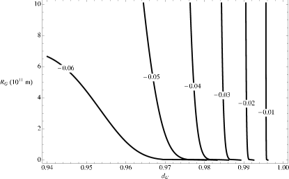
Figure 1: Contour plot of $T_{r}-1$ in function of $R_{G}$ and $d_{U}$.

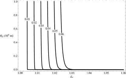
Figure 2: Contour plot of $T_{r}-1$ in function of $\log R_{G}$ and $d_{U}$.

Numerical solutions of Eq. (15) allow for obtaining contour plots for $T_{r}-1$ as a function of $d_{U}$ and $\xi_{G}$. The results are depicted in Figs. 1 and 2 for $|T_{r}-1|\leq 0.06$, the uncertainty in the Sun’s central temperature Bhatia .

Designating the line in Fig. 1 that indicates a $6\%$ change of the Sun’s central temperature as $R_{-}(d_{U})$, one sees that $R_{G}(d_{U})>R_{-}(d_{U})$ for $d_{U}\lesssim 1$. Thus, Eq. (I) leads to

$${M_{*}\over M_{Pl}}>\left[\pi\Lambda_{U}R_{-}(d_{U})\right]^{1-d_{U}}f(d_{U},\alpha)~{}~{},$$ (18)

where

$$f(d_{U},\alpha)=\sqrt{{2(2-\alpha)\over\pi}{\Gamma(d_{U}+{1\over 2})\Gamma(d_{U}-{1\over 2})\over\Gamma(2d_{U})}}~{}~{}$$ (19)

is defined, for convenience. One might plot the lower bound obtained above as a function of $d_{U}$, fixing the model parameters $\alpha$ and $\Lambda_{U}$. This is depicted in Fig. 3, for $\alpha=0,~{}2/3,~{}1,~{}1.9$ and suitable values for $\Lambda_{U}$; all lines converge to the trivial point $d_{U}=1,M_{*}\geq 0$.

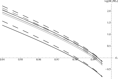
Figure 3: Lower bound of $\log(M_{*}/M_{Pl})$ for $\alpha=0$ (black curve), $\alpha=2/3$ (dark grey curve), $\alpha=1$ (light grey curve), $\alpha=1.9$ (black, lower curve), and $\Lambda_{U}=1~{}TeV$ (solid curve), $\Lambda_{U}=10^{3}~{}TeV$ (dashed curve).

Similarly, one obtains from Fig. 2 the upper bound $R_{G}(d_{U})<R_{+}(d_{U})$, where the latter denotes the line corresponding to the $6\%$ change in the Sun’s central temperature. Resorting again to Eq. (I), this again yields

$${M_{*}\over M_{Pl}}>\left[\pi\Lambda_{U}R_{+}(d_{U})\right]^{1-d_{U}}f(d_{U},\alpha)~{}~{}.$$ (20)

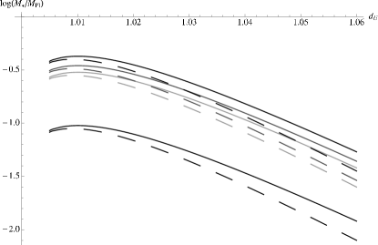
Figure 4: Lower bound of $\log(M_{*}/M_{Pl})$ for $\alpha=0$ (black curve), $\alpha=2/3$ (dark grey curve), $\alpha=1$ (light grey curve), $\alpha=1.9$ (black, lower curve), and $\Lambda_{U}=1~{}TeV$ (solid curve), $\Lambda_{U}=10^{3}~{}TeV$ (dashed curve).

The obtained lower bound is depicted in Fig. 4 (as before, the lines converge to the point $d_{U}=1,M_{*}\geq 0$).

IV.1 Discussion

As stated in Ref. ungravity , corrections to the Newtonian potential $\Phi_{N}(r)$ with $d_{U}<1$ might appear unfeasible, since these will overcome the $1/r$ dependence of $\Phi_{N}(r)$ for $r>R_{g}$ and lead to long-range deviations. This might be alleviated by letting $R_{G}$ be so large that this crossover occurs well beyond the relevant astrophysical range, and one can no longer assume a static, spherically symmetric Ansatz for the metric.

Alternatively, one may consider values so close to unity, $d_{U}\lesssim 1$, that the perturbation to the Newtonian potential, Eq. (6) may be expanded as $(r/R_{G})^{2-2d_{U}}\approx 1+2(d_{U}-1)\log(r/R_{g})$, and the logarithmic dependence is attenuated by the small $d_{U}-1$ term: for instance, for $r=100~{}AU$, the typical dimension of the Solar System and $R_{G}\sim 10~{}AU$, the maximum value considered here, this yields $(r/R_{G})^{2-2d_{U}}\approx 1+4(d_{U}-1)$; assuming the same value for $R_{G}$ and instead, if $r\sim 100~{}kpc\sim 10^{10}~{}AU$ the size of a galaxy, one still gets $(r/R_{G})^{2-2d_{U}}\approx 1+20(d_{U}-1)$.

With these considerations in mind, the method developed here shows that one can successfully constrain the range of $M_{U}$ for $d_{U}\lesssim 1$: in particular, assuming $\Lambda_{U}\geq 1~{}TeV$ one achieves lower bounds ranging from $M_{*}\gtrsim(10^{-1}-10^{2})M_{Pl}$ (even lower bounds can be obtained for values of $d_{U}$ closer to unity).

For the case $d_{U}\gtrsim 1$, one obtains a lower bound exhibiting a peak around $d_{U}=1.01$, with typical values $M_{*}\gtrsim(10^{-2}-10^{-1})M_{Pl}$. Ref. ungravity presents lower bounds for $M_{*}$ as a function of $\Lambda_{U}$, for $d_{U}=2,~{}3,~{}4$ — values which are beyond the reach of this study. In a subsequent study, the cases $d_{U}=1.1,~{}1.5,~{}2$ were considered, with the first case closer to the range considered here cosmo .

By solving Eq. (15) for $d_{U}=1.1$ and finding the value of $R_{G}$ that yields $T_{r}-1=0.06$, one obtains a lower bound of about $M_{*}>(10^{-4}-10^{-2})M_{Pl}\approx(10^{12}-10^{14})~{}TeV$, depending on $\Lambda_{U}$ and $M_{*}$ (this may be checked by extrapolating the plot of Fig. 2). This limit is much greater than the one found in Ref. cosmo , where a result $M_{*}\gtrsim(10^{2}-10^{6})~{}TeV$ is reported (for $\Lambda_{U}=10^{6}~{}TeV$). This indicates that the developed method hints at a much more stringent bound for $M_{*}$, for $d_{U}\gtrsim 1$.

V Conclusions

In this work we have set up a formalism to constrain ungravity-inspired deviations from the Newtonian hydrostatic equilibrium conditions within a star. This leads to a perturbed Lane-Emden problem that is then examined for the polytropic index $n=3$. From the resulting change in the star’s central temperature, we obtain constraints on the ungravity parameters $R_{G}$ and $d_{U}$. Given that the overall properties of the Sun are well described by the $n=3$ case, we allow for the ungravity correction to affect this up to the upper bound on the Sun’s central temperature, $\Delta T_{c}/T_{c}\approx 0.06$.

We find that, for $d_{U}\gtrsim 1$ and $\Lambda_{U}\geq 1~{}TeV$, lower bounds on $M_{*}$ are in the range $(10^{-2}-10^{-1})M_{Pl}$. For $d_{U}\lesssim 1$ and $\Lambda_{U}\geq 1~{}TeV$, $M_{*}$ must lie in the range above $(10^{-1}-10^{2})M_{Pl}$. Of course, our bounds are complementary to the ones obtained from torsion balance experiments which test a much smaller range of $R_{G}$ searches , actually about $80~{}\mu m$.

The reported results for $d_{U}\gtrsim 1$ are either more stringent cosmo0 ; freitas ; cosmo ; hsu ; mureika or similar das to those previously available. The lower bound derived for $d_{U}\lesssim 1$ is more relevant, since it has been not obtained so far. In our opinion, this arises from misconception that a negative exponent in Eq. (6) is disallowed by long-range experiments searches : while this is true for large values of $1-d_{U}$, a range closer to unity, $d_{U}\lesssim 1$ yields an approximately logarithmic correction, with large deviations from the Newtonian potential suppressed by the smallness of the $d_{U}-1$ term.

- (1) H. Georgi, Phys. Rev. Lett. 98, 221601 (2007).
- (2) H. Goldberg and P. Nath, Phys. Rev. Lett. 100, 031803 (2008).
- (3) O. Bertolami and J. Páramos, Phys. Rev. D 72, 044001 (2005).
- (4) H. Davoudiasl, Phys. Rev. Lett. 99, 141301 (2007).
- (5) A. Freitas and D. Wyler, JHEP 0712, 033 (2007).
- (6) S. Das, S. Mohanty and K. Rao, Phys. Rev. D 77, 076001 (2008).
- (7) N. G. Deshpande, S. D. H. Hsu and J. Jiang, Phys. Lett. B 659, 888 (2008).
- (8) J. R. Mureika, Phys. Lett. B 660, 561 (2008); Phys. Rev. D 79, 056003 (2009).
- (9) J. McDonald, JCAP 0903, 019 (2009).
- (10) O. Bertolami and N. M. C. Santos, Phys. Rev. D 79, 127702 (2009).
- (11) O. Bertolami and J. Páramos, Phys. Rev. D 71, 023521 (2005).
- (12) O. Bertolami and J. Páramos, Phys. Rev. D 77, 084018 (2008).
- (13) Textbook of Astronomy and Astrophysics with Elements of Cosmology, V. Bhatia (Narosa Publishing House, New Delhi, 2001).
- (14) E. G. Adelberger, B. R. Heckel, S. A. Hoedl, C. D. Hoyle, D. J. Kapner and A. Upadhye, Phys. Rev. Lett. 98, 131104 (2007).