Liquid crystals and harmonic maps in polyhedral domains

Abstract

Unit-vector fields ${\bf n}$ on a convex polyhedron $P$ subject to tangent boundary conditions provide a simple model of nematic liquid crystals in prototype bistable displays. The equilibrium and metastable configurations correspond to minimisers and local minimisers of the Dirichlet energy, and may be regarded as $S^{2}$-valued harmonic maps on $P$. We consider unit-vector fields which are continuous away from the vertices of $P$. A lower bound for the infimum Dirichlet energy for a given homotopy class is obtained as a sum of minimal connections between fractional defects at the vertices of $P$. In certain cases, this lower bound can be improved by incorporating certain nonabelian homotopy invariants. For a rectangular prism, upper bounds for the infimum Dirichlet energy are obtained from locally conformal solutions of the Euler-Lagrange equations, with the ratio of the upper and lower bounds bounded independently of homotopy type. However, since the homotopy classes are not weakly closed, the infimum may not be realised; the existence and regularity properties of continuous local minimisers of given homotopy type are open questions. Numerical results suggest that some homotopy classes always contain smooth minimisers, while others may or may not depending on the geometry of $P$. Numerical results modelling a bistable device suggest that the observed nematic configurations may be distinguished topologically.

This article appears as a chapter in “Analysis and Stochastics of Growth Processes and Interface Models”, P Morters et al. eds., Oxford University Press 2008, http://www.oup.com/uk/catalogue/?ci=9780199239252.

1 Introduction

Liquid crystals are intermediate phases of matter exhibiting partial ordering in the orientation and/or positions of their constituent particles. The constituents of nematic liquid crystals have a distinguished axis, and in the nematic phase these axes tend to align. The direction and degree of alignment can exhibit a rich variety of singularities. Standard references on liquid crystals include [3, 23, 9, 21].

The nematic phase is optically birefringent (light propagation is polarisation-dependent). This, together with the fact that nematic ordering can be modified by external electric and magnetic fields, has led to a wide range of display applications. Most present-day liquid crystal displays (eg twisted nematic) are based on monostable cells, where, in the absence of external fields, the orientation assumes a single (spatially varying) equilibrium configuration which is effectively transparent to incident polarised light. To produce and maintain optical contrast, voltage pulses, which change the orientation, must be continually applied. There is considerable interest in developing bistable cells, which support two (and possibly more) stable configurations with contrasting optical properties. In bistable cells, power is needed only to switch between configurations. One mechanism for engendering bistability is to introduce microstructures into the geometry [7, 8, 22]. Nematic liquid crystals in cells with polyhedral features (eg, ridges, posts, wells) have been found to support multiple configurations. One such device, the PABN, or post-aligned bistable nematic cell, is shown in Fig. 1 ([8]). It consists of a liquid crystal layer sandwiched between two planar substrates, with the lower substrate featured by an array of microscopic posts.

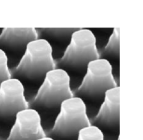
Figure 1: The PABN cell (from [8])

As a simple model for such systems, we consider nematic liquid crystals in a convex polyhedron $P\subset{\mathbb{R}}^{3}$ with orientation described by a director field, ${\bf n}:P\rightarrow RP^{2}$, taking values in the real projective plane. We consider the case of strong azimuthal anchoring, described by tangent boundary conditions. Tangent boundary conditions require that, on a face of $P$, ${\bf n}$ lies tangent to the face, but is otherwise unconstrained. It follows that on the edges of $P$, ${\bf n}$ is parallel to the edges, and therefore is necessarily discontinuous at the vertices. We are interested as to whether equilibria can be classified according to homotopy, and therefore restrict our attention to director fields which are continuous away from the vertices. For these, we can unambiguously assign an orientation to the director field (as $P$ is simply connected), and regard ${\bf n}$ as a unit-vector field. We let $C_{T}^{0}(P,S^{2})$ denote the space of continuous unit-vector fields on $P$ satisfying tangent boundary conditions, or tangent unit-vector fields for short.

The elastic or Oseen-Frank energy of a configuration ${\bf n}$ is given by

$$E=\int_{P}\big{[}K_{1}({\bf\nabla}\cdot{\bf n})^{2}+K_{2}({\bf n}\cdot({\bf\nabla}\times{\bf n}))^{2}+K_{3}({\bf n}\times({\bf\nabla}\times{\bf n}))^{2}\\ +K_{4}{\bf\nabla}\cdot(({\bf n}\cdot{\bf\nabla}){\bf n}-({\bf\nabla}\cdot{\bf n}){\bf n})\big{]}\,dV.$$ (1)

Tangent boundary conditions imply that the contribution from the $K_{4}$-term, which is a pure divergence, vanishes. We shall make use of the so-called one-constant approximation, in which the remaining elastic constants $K_{1}$, $K_{2}$ and $K_{3}$ are taken to be the same and set to unity. In this case, (1) becomes the Dirichlet energy,

$$E({\bf n})=\int_{P}({\bf\nabla}{\bf n})^{2}\,dV.$$ (2)

Minimisers of the Dirichlet energy, which correspond to equilibrium configurations, are $S^{2}$-valued harmonic maps, as are local minimisers, which correspond to metastable configurations.

The homotopy classes of $C_{T}^{0}(P,S^{2})$ are described in Section 2, and a lower bound for the infimum of the Dirichlet energy in each homotopy class is given in Section 3. The lower bound is expressed as a sum of minimal connections between fractional defects at the vertices of $P$, in analogy with the well-known result of [2] for the infimum Dirichlet energy of a set of point defects in ${\mathbb{R}}^{3}$. For nonconformal homotopy classes, this bound can be improved by incorporating certain nonabelian homotopy invariants; this is shown explicitly for certain homotopy classes in a rectangular prism in Section 4. Unlike the case of point defects in ${\mathbb{R}}^{3}$, the lower bound of Section 3 is expected to be strictly less than the infimum; achieving the lower bound would require concentration along a minimal connection, which would be incompatible with tangent boundary conditions. However, for $P$ a rectangular prism, we can construct trial configurations in each homotopy class whose energies differ from the lower bound by a factor which is bounded independently of $h$ (Section 5). Generalising the construction to arbitrary $P$ requires finding conformal maps on $S^{2}$ which preserve a given set of geodesics.

It is an open question as to whether the infimum is achieved in a given homotopy class, as is the regularity of the local minimisers. Numerical results presented in Section 6 suggest that some homotopy classes always contain smooth minimisers, while others may or may not depending on the geometry of $P$. Numerical results for a model of a bistable display suggests that the observed nematic configurations are topologically distinct.

In addition to existence and regularity questions, it would be interesting to investigate namics under the influence of applied fields. Switching between configurations of different homotopy type requires the creation and destruction of defects, and one would like to understand this process in detail.

2 Homotopy classification

Given ${\bf n}\in C_{T}^{0}(P,S^{2})$ we can identify a number of discrete-valued quantities which depend continuously on ${\bf n}$ and which are therefore homotopy invariants. (Details may be found in [18] and [16]). Along an edge of $P$, ${\bf n}$ must lie parallel to the edge, so its value there is determined up to a sign, which we call an edge orientation (see Fig. 2(a)). Next, along a path on a face of $P$ between two edges, ${\bf n}$ must lie tangent to the face, and therefore describes a geodesic on $S^{2}$, ie an arc of a great circle (see Fig. 2(b)). As the endpoints of the geodesic are fixed by the edge orientations, the geodesic may be assigned an integer-valued relative winding number, or kink number. By convention, the shortest geodesic is assigned kink number zero. Another invariant is associated with a surface which separates one of the vertices of $P$ from the other vertices – we call this a cleaved surface (see Fig. 2(c)). Along the boundary of a cleaved surface, ${\bf n}$ is determined up to homotopy by its edge orientations and kink numbers. Therefore, the signed area of the image of the cleaved surface itself, called the trapped area at the vertex, is determined up to an integer multiple of $4\pi$ (ie, some number of whole coverings of the sphere).

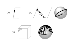
Figure 2: Homotopy invariants. (a) Edge orientation (b) Kink number. ${\bf n}$ describes a 3/4-turn about the vertex (the image on $S^{2}$ is also shown), corresponding to kink number $-1$. (c) Trapped area. The image of the cleaved surface on $S^{2}$ has signed area $-3\pi/2$.

Collectively, the edge orientations, kink numbers and trapped areas constitute a complete set of homotopy invariants for $C_{T}^{0}(P,S^{2})$; two configurations are homotopic if and only if their invariants are the same. We note that the invariants are not all independent – continuity of configurations on the faces of $P$ implies that the kink numbers on each face satisfy a sum rule, while continuity on the interior of $P$ implies that the trapped areas add up to zero. One can show that every set of invariants satisfying these sum rules can be realised.

From the preceding discussion, it is evident that the invariants of ${\bf n}$ can be determined from its values on a set of cleaved surfaces (the values of ${\bf n}$ on the corners and edges of the cleaved surfaces determine its edge orientations and kink numbers). Given a set of cleaved surfaces we can define an alternative set of invariants, the wrapping numbers, which will be used in subsequent sections. Let $T\subset S^{2}$ denote the set of directions which are tangent to one of the faces of $P$. Then $T$ consists of a union of great circles. $S^{2}-T$ consists of a union of disjoint open spherical polygons, which we call sectors (see Fig. 3). Let $C^{a}$ denote a cleaved surface separating the $a$th vertex of $P$, say, from the others, and let ${\bf n}^{a}$ denote the restriction of ${\bf n}$ to $C^{a}$. Let $\Sigma^{\sigma}$ denote the $\sigma$th sector of $S^{2}$. The wrapping number $w^{a\sigma}$ is the number of times ${\bf n}^{a}$ covers $\Sigma^{\sigma}$, counted with orientation. For ${\bf n}$ differentiable, this is given by

$$w^{a\sigma}=\frac{1}{A^{\sigma}}\int_{C^{a}}\,{\bf n}^{*}(\chi^{\sigma}\omega),$$ (3)

where $\omega$ is the area two-form on $S^{2}$, normalised to have integral $4\pi$, $\chi^{\sigma}$ is the characteristic function of $\Sigma^{\sigma}$, ${\bf n}^{*}$ denotes the pull-back, and $A^{\sigma}=\left|\int_{S^{2}}\chi^{\sigma}\,\omega\right|$ is the area of $\Sigma^{\sigma}$. Alternatively, $w^{a\sigma}$ can be expressed as the index of a regular value ${\bf s}\in\Sigma^{\sigma}$, ie

$$w^{a\sigma}=\sum_{{\bf r}\,|\,{\bf n}^{a}({\bf r})={\bf s}}\text{sgn}\,\det({\bf n}^{a})^{\bf{}^{\prime}}({\bf r}).$$ (4)

The wrapping numbers are homotopy invariants, and using Stokes’ theorem can be expressed in terms of the edge orientations, kink numbers and trapped areas. These relations can also be inverted to obtain the edge orientations, kink numbers and trapped areas in terms of the wrapping numbers. Thus, the wrapping numbers constitute a complete (though redundant) set of homotopy invariants.

If the nonzero wrapping numbers at a given vertex are all negative, the homotopy class is said to be conformal with respect to that vertex, and if positive, anticonformal with respect to that vertex. A homotopy class is called nonconformal if there are vertices with wrapping numbers of different signs.

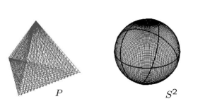
Figure 3: Sectors for a tetrahedron. The great circles of directions tangent to the four faces partition the two-sphere into 14 sectors.

It is straightforward to count the number of invariants as well as the relations among them. Suppose that $P$ has $f$ faces, $e$ edges and $v$ vertices (so that, from Euler’s formula, $f-v+e=2$). Then $P$ has $v$ trapped areas, which satisfy a single sum rule; $2e$ kink numbers, which satisfy $f$ sum rules; and $e$ edge orientations. It also follows from Euler’s formula applied to the set of tangent directions $T$, regarded as a graph on $S^{2}$, that there are generically (and at most) $f^{2}-f+2$ sectors (‘generically’ means that no direction is tangent to three or more faces of $P$). Thus, there are generically (and at most) $(f^{2}-f+2)v$ wrapping numbers, many more than the number of trapped areas and kink numbers. Among the constraints on the wrapping numbers, we point out that for a fixed sector $\Sigma^{\sigma}$, their sum over vertices must vanish, ie

$$\sum_{a}w^{a\sigma}=0.$$ (5)

We will use $h$ to denote both an admissible set of values of the invariants as well as the homotopy class in $C^{0}_{T}(P,S^{2})$ characterised by these values.

3 Lower bound: minimal connection

[2] established the infimum Dirichlet energy for unit-vector fields on ${\mathbb{R}}^{3}$ with point defects of specified position and degree. The result is expressed in terms of a minimal connection between the defects, defined below. A similar argument yields a lower bound for the infimum Dirichlet energy for tangent unit-vector fields on $P$ of fixed homotopy type, in which the vertices of $P$ play the role of defects, and the wrapping numbers that of generalised degrees. Details may be found in [14], [13], and [16].

We first review the result of [2]. Let $\Omega={\mathbb{R}}^{3}-\{{\bf r}^{1},\ldots,{\bf r}^{n}\}$, and let ${\bf n}:\Omega\rightarrow S^{2}$ denote a unit-vector field on $\Omega$. Continuous unit-vector fields on $\Omega$ may be classified up to homotopy by their degrees, $d=(d^{1},\ldots,d^{n})\in{\mathbb{Z}}^{n}$, on spheres about each of the excluded points ${\bf r}_{j}$ (the restriction of ${\bf n}$ to such a sphere may be regarded as a map from $S^{2}$ into itself). For ${\bf n}$ smooth,

$$d^{j}=\frac{1}{4\pi}\int_{|{\bf r}-{\bf r}^{j}|=\epsilon}{\bf n}^{*}\omega$$ (6)

for small enough $\epsilon$. For ${\bf\nabla}{\bf n}$ square-integrable, the Dirichlet energy is given as in (2) by

$$E({\bf n})=\int_{\Omega}({\bf\nabla}{\bf n})^{2}dV.$$ (7)

In order for $E({\bf n})$ to be finite, we require that

$$\sum_{j}d^{j}=0.$$ (8)

Let $C^{0}_{\Omega}(d)$ denote the homotopy class of continuous unit-vector fields with degrees $d$ satisfying (8), and let

$$E^{\text{inf}}_{\Omega}(d)=\inf_{{\bf n}\in C^{0}_{\Omega}(d)\cap H^{1}(\Omega,S^{2})}E({\bf n})$$ (9)

denote the infimum energy in $C^{0}_{\Omega}(d)$.

Given two $m$-tuples of points in ${\mathbb{R}}^{3}$, ${\cal P}=({\bf a}^{1},\ldots,{\bf a}^{m})$ and ${\cal N}=({\bf b}^{1},\ldots,{\bf b}^{m})$ (whose points need not be distinct), a connection is a pairing $({\bf a}^{j},{\bf b}^{\pi(j)})$ of points in ${\cal P}$ and ${\cal N}$, specified here in terms of a permutation $\pi\in S_{m}$ ($S_{m}$ denotes the symmetric group). The length of a connection is the sum of the distances between the paired points, and a minimal connection is a connection of minimum length. Let

$$L({\cal P},{\cal N})=\min_{\pi\in S_{m}}\sum_{j=1}^{m}|{\bf a}^{j}-{\bf b}^{\pi(j)}|$$ (10)

denote the length of a minimal connection, and let $|d|={\textstyle\frac{1}{2}}\sum_{j}|d^{j}|$.

Theorem 3.1

[2] The infimum $E^{\text{inf}}_{\Omega}(d)$ of the Dirichlet energy of continuous unit-vector fields on the domain $\Omega={\mathbb{R}}^{3}-\{{\bf r}^{1},\ldots,{\bf r}^{n}\}$ of degrees $d^{j}$ about the excluded points ${\bf r}^{j}$ is given by

$$E^{\text{inf}}_{\Omega}(d)=8\pi L({\cal P}(d),{\cal N}(d)),$$ (11)

where ${\cal P}(d)$ is the $|d|$-tuple of excluded points of positive degree, with ${\bf r}^{j}$ included $d^{j}$ times, and $N(d)$ is the $|d|$-tuple of excluded points of negative degree, with ${\bf r}^{k}$ included $|d^{k}|$ times.

In fact, the result of [2] applies to more general domains with holes.

Here we sketch the argument that $8\pi L({\cal P}(d),{\cal N}(d))$ is a lower bound for $E^{\text{inf}}_{\Omega}(d)$. It suffices to consider smooth unit-vector fields on $\Omega$, as these are dense in $C^{0}_{\Omega}(d)\cap H^{1}(\Omega,S^{2})$. For any orthonormal frame ${\bf u}$, ${\bf v}$, ${\bf w}$, one has the inequality

$$({\bf\nabla}{\bf n})^{2}\geq 2|(d\xi\wedge{\bf n}^{*}\omega)({\bf u},{\bf v},{\bf w})|\geq 2(d\xi\wedge{\bf n}^{*}\omega)({\bf u},{\bf v},{\bf w}),$$ (12)

where $\xi$ is differentiable and $|d\xi|\leq 1$. (12) follows from the fact that, at every point, there is at least one direction (say ${\bf u}$) in which the directional derivative $\nabla_{u}{\bf n}:=({\bf u}\cdot{\bf\nabla}){\bf n}$ vanishes, while

$$(\nabla_{v}{\bf n})^{2}+(\nabla_{w}{\bf n})^{2}\geq 2|\nabla_{v}{\bf n}|\,|\nabla_{w}{\bf n}|\geq 2|\nabla_{v}{\bf n}\wedge\nabla_{w}{\bf n}|.$$ (13)

Since $d\omega=0$, it follows that $d\xi\wedge{\bf n}^{*}\omega=d(\xi{\bf n}^{*}\omega)$, so that

$$({\bf\nabla}{\bf n})^{2}\geq 2d(\xi{\bf n}^{*}\omega).$$ (14)

Substituting (14) into (7) and applying Stokes’ theorem, we get a lower bound

$$E^{\text{inf}}_{\Omega}(d)\geq 2\sum_{j}\xi^{j}d^{j},$$ (15)

which depends only on the values $\xi^{j}:=\xi({\bf r}^{j})$ of $\xi$ at the defects. Since $|d\xi|\leq 1$, these values are constrained by $|\xi^{j}-\xi^{k}|\leq|{\bf r}^{j}-{\bf r}^{k}|$. In fact, every set of $\xi^{j}$’s satisfying these constraints can be realised by a piecewise-differentiable function $\xi$ (eg, let $\xi({\bf r})=\max_{j}(\xi^{j}-|{\bf r}-{\bf r}^{j}|)$). Thus, one obtains a bound

$$E^{\text{inf}}_{\Omega}(d)\geq 2\max_{\xi^{j}}\sum_{j}\xi^{j}d^{j},\ \text{where}\ \xi^{j}\geq 0,\ |\xi^{j}-\xi^{k}|\leq|{\bf r}^{j}-{\bf r}^{k}|,$$ (16)

in the form of a finite-dimensional linear optimisation problem.

The dual formulation is given by

$$E^{\text{inf}}_{\Omega}(d)\geq 2\min_{\eta_{jk}}\sum_{jk}\eta_{jk}|{\bf r}^{j}-{\bf r}^{k}|,\ \text{where}\ \eta_{jk}\geq 0,\sum_{k}(\eta_{jk}-\eta_{kj})\geq d^{j}.$$ (17)

This is a sort of transport problem, in which the degrees are the quantities to be transported and the costs are the distances between defects. We can take $\eta_{jk}$ to be $0$ unless $d^{j}>0$ and $d^{k}<0$. Without loss of generality, we may also assume that the degrees are either $+1$ or $-1$, so that there are an equal number, $m:=n/2$, of each, with positions $({\bf a}^{1},\ldots,{\bf a}^{m})$ and $({\bf b}^{1},\ldots,{\bf b}^{m})$ respectively (if not, repeat each defect according to its multiplicity). (17) becomes

$$E^{\text{inf}}_{\Omega}(d)\geq 2\min_{M_{pq}}\sum_{p,q=1}^{m}M_{pq}|{\bf a}^{p}-{\bf b}^{q}|,\ \text{where}\ M_{pq}\geq 0,\sum_{p}M_{pq}=\sum_{q}M_{qp}=1.$$ (18)

As $M$ is constrained to be doubly stochastic, a theorem of Birkhoff [1] implies that it lies in the convex hull of the set of $m$-dimensional permutation matrices. The optimal solution will be amongst the permutation matrices themselves, leading to $E^{\text{inf}}_{\Omega}(d)\geq 8\pi L({\cal P}(d),{\cal N}(d))$.

A similar argument leads to a lower bound for the infimum Dirichlet energy for tangent unit-vector fields on $P$ of given homotopy type.

Theorem 3.2

[16] Let $h=\{w^{a\sigma}\}$ be an admissible topology for continuous tangent unit-vector fields on a polyhedron $P$. The infimum $E^{\text{inf}}(h)$ of the Dirichlet energy of continuous tangent unit-vector fields on $P$ with invariants $h$ is bounded below by

$$E^{\text{inf}}_{P}(h)\geq\sum_{\sigma}2A^{\sigma}L({\cal P}^{\sigma}(h),{\cal N}^{\sigma}(h)),$$ (19)

where ${\cal P}^{\sigma}$ (resp. ${\cal N}^{\sigma}$) contains the vertices of $P$ for which $w^{a\sigma}$ is positive (resp. negative), each such vertex included with multiplicity $|w^{a\sigma}|$.

Thus, to each sector $\sigma$ may be associated a constellation of point defects at the vertices ${\bf v}^{a}$ with degrees $w^{a\sigma}$. The lower bound of (19) is a sum of the lengths of minimal connections for these constellations, weighted by the sector areas $A^{\sigma}$.

4 Lower bound: nonabelian invariants

For nonconformal homotopy classes, the lower bound of Theorem 3.2 can be improved by incorporating certain nonabelian invariants. These invariants, and the sense in which they are nonabelian, are introduced in Section 4.1 in a two-dimensional setting. For tangent unit-vector fields on $P\subset{\mathbb{R}}^{3}$ we describe this phenomenon in a particular case (Section 4.2), reflection-symmetric homotopy classes in a rectangular prism. Details will be given in [15].

4.1 Absolute degree and spelling length

Let $\phi:D^{2}\rightarrow{\mathbb{R}}^{2}$ be a smooth map of the two-disk into the plane. We recall that $x\in D^{2}$ is a regular point of $\phi$ if $x$ is in the interior of $D^{2}$ and $\det\phi^{\prime}(x)\neq 0$, $y\in{\mathbb{R}}^{2}$ is regular value of $\phi$ if all of its preimages are regular points, and a regular value has a finite number of preimages. Let ${\cal R}(\phi)\subset{\mathbb{R}}^{2}$ denote the set of regular values of $\phi$. From Sard’s theorem, $\,\text{Im}\,\phi-{\cal R}(\phi)$ is of zero measure.

Given $y\in{\cal R}(\phi)$, the algebraic degree of $y$ (or degree, for short) is given by

$$d_{\phi}(y)=\sum_{x\in\phi^{-1}(y)}\text{sgn}\,\det\phi^{\prime}(x),$$ (20)

and is invariant under smooth deformations of $\phi$ which preserve the boundary map $\partial\phi$. We define the absolute degree of $y$ by

$$D_{\phi}(y)=\sum_{x\in\phi^{-1}(y)}1.$$ (21)

Clearly $D_{\phi}(y)$ is not invariant under all deformations which preserve $\partial\phi$, and

$$D_{\phi}(y)\geq|d_{\phi}(y)|.$$ (22)

Let $R=\{y_{1},\ldots,y_{n}\}\subset{\cal R}(\phi)$ denote a set of $n$ regular values of $\phi$. We may regard the boundary $\partial\phi$ as a map $\partial\phi:S^{1}\rightarrow{\mathbb{R}}^{2}-R$ from the circle to the $n$-times-punctured plane. Let $\pi_{1}({\mathbb{R}}^{2}-R,p)$ denote the fundamental group of ${\mathbb{R}}^{2}-R$, based at a point $p$, and let $[\partial\phi]\in\pi_{1}({\mathbb{R}}^{2}-R,p)$ denote the homotopy class of $\partial\phi$.

The fundamental group $\pi_{1}({\mathbb{R}}^{2}-R,p)$ may be identified with the free group on $n$ generators, $F(c_{1},\ldots,c_{n})$ (see, eg, [10]). Let us specify that the generator $c_{j}$ corresponds to a loop which encircles $y_{j}$ once with positive orientation but contains no other $y_{k}$’s. This determines the $c_{j}$’s up to conjugacy. Given $g\in\pi_{1}({\mathbb{R}}^{2}-R,p)$, we define a spelling to be a factorisation of $g$ into a product of conjugated generators and inverse generators, eg

$$g=h_{1}c_{i_{1}}^{\epsilon_{1}}h_{1}^{-1}\cdots h_{r}c_{i_{r}}^{\epsilon_{r}}h_{r}^{-1},$$ (23)

where $h_{s}\in\pi_{1}({\mathbb{R}}^{2}-R,p)$ and $\epsilon_{s}=\pm 1$. The length of a spelling is the number of factors (ie, $r$ in (23)). Define the spelling length, denoted $\Lambda_{n}(g)$, to be the shortest possible length of a spelling of $g$ (eg, $\Lambda_{n}(c_{1}c_{2}c_{1}^{-1}c_{2}^{-1})=2$). The spelling length of the identity, $e$, is taken to be zero. It turns out that the spelling length of $[\partial\phi]$ gives a lower bound on the sum of the absolute degrees of points in $R$.

Proposition 4.1

Given $\phi:D^{2}\rightarrow{\mathbb{R}}^{2}$ smooth, $R=\{y_{1},\ldots,y_{n}\}\subset{\cal R}(\phi)$, and $\pi_{1}({\mathbb{R}}^{2}-R,p)\backsimeq F_{n}(c_{1},\ldots,c_{n})$, with generators $c_{j}$ as above. Then

$$\sum_{j=1}^{n}D_{\phi}(y_{j})\geq\Lambda_{n}([\partial\phi]).$$ (24)

Let $\bar{F}_{n}(c_{1},\ldots,c_{n})$ denote the abelianisation of $F_{n}(c_{1},\ldots,c_{n})$, obtained by taking all of the $c_{j}$’s to commute, and given $g\in F_{n}(c_{1},\ldots,c_{n})$, let $\bar{g}$ denote the corresponding element of $\bar{F}_{n}(c_{1},\ldots,c_{n})$. Then $\bar{g}$ can be written as $c_{1}^{\delta_{1}}\cdots c_{n}^{\delta_{n}}$ for some integers $\delta_{j}$. Let $\bar{\Lambda}_{n}(g)=\sum_{j=1}^{n}|\delta_{j}|$ . Clearly $\Lambda_{n}(g)\geq\bar{\Lambda}_{n}(g)$ (eg, $\bar{\Lambda}_{n}(c_{1}c_{2}c_{1}^{-1}c_{2}^{-1})=0)$. It is readily seen that

$$\sum_{j=1}^{n}|d_{\phi}(y_{j})|=\bar{\Lambda}_{n}([\partial\phi]).$$ (25)

Thus, Proposition 4.1 implies that $\sum_{j}D_{\phi}(y_{j})$ is strictly greater than $\sum_{j}|d_{\phi}(y_{j})|$ provided that $\Lambda_{n}([\partial\phi])$ is strictly greater than $\bar{\Lambda}_{n}([\partial\phi])$. For example, if $[\partial\phi]=c_{1}c_{2}c_{1}^{-1}c_{2}^{-1}$, then $\phi$ takes values $y_{1}$ or $y_{2}$ at least twice, even though $y_{1}$ and $y_{2}$ are of degree zero.

For our applications we shall want to consider maps ${\boldsymbol{\nu}}:D^{2}\rightarrow S^{2}$ from the two-disk into the two-sphere. Let $R=\{{\bf e}_{0},\ldots,{\bf e}_{n}\}\in{\cal R}({\boldsymbol{\nu}})$ denote a set of $n+1$ regular values of ${\boldsymbol{\nu}}$. In contrast to the case of maps to the plane, the algebraic degrees $d({\bf e}_{j})$ are not determined by $\partial{\boldsymbol{\nu}}$, since the image of ${\boldsymbol{\nu}}$ itself is determined only up to whole coverings of $S^{2}$. We can remove this ambiguity by specifying the degree at one of the regular values, eg $d_{\boldsymbol{\nu}}({\bf e}_{0})=d_{0}$. We may identify the fundamental group $\pi_{1}(S^{2}-R,{\bf q})$ with the free group $F_{n}(c_{1},\ldots,c_{n})$ on $n$ generators. As above, we specify that the generator $c_{j}$ corresponds to a closed loop which encircles ${\bf e}_{j}$ once with positive orientation but contains no other ${\bf e}_{k}$’s, which determines the $c_{j}$’s up to conjugacy. $c_{0}$, which corresponds to a loop about ${\bf e}_{0}$, may be expressed as a product of the generators $c_{1}$ through $c_{n}$ and their inverses. In what follows, we write $b\sim c$ to denote that $b$ and $c$ are conjugate. In analogy with Proposition 4.1, we have the following:

Proposition 4.2

Given ${\boldsymbol{\nu}}:D^{2}\rightarrow S^{2}$ smooth, $R=\{{\bf e}_{0},\ldots,{\bf e}_{n}\}\subset{\cal R}({\boldsymbol{\nu}})$, and $\pi_{1}({\mathbb{R}}^{2}-R,p)\backsimeq F_{n}(c_{1},\ldots,c_{n})$ with generators $c_{j}$ as above, such that $c_{0}\in F_{n}(c_{1},\ldots,c_{n})$. Suppose that $d_{\boldsymbol{\nu}}({\bf e}_{0})=d_{0}$. Then

$$\sum_{j=0}^{n}D_{{\boldsymbol{\nu}}}({\bf e}_{j})\geq|d_{0}|+\min_{\begin{subarray}{c}g_{1},\ldots,g_{r+|d_{0}|}\sim c_{0},\\ h_{1},\ldots,h_{r}\sim c_{0}^{-1}\end{subarray}}\Lambda_{n}([\partial{\boldsymbol{\nu}}]g_{1}\cdots g_{r+|d_{0}|}h_{1}\cdots h_{r}).$$ (26)

While it is straightforward to compute the spelling length of a given element $g$, evaluating (26) may not be as straightforward.

4.2 Reflection-symmetric homotopy classes in a prism

A crude way to obtain a lower bound for the Dirichlet energy of tangent unit-vector fields on $P$ is to estimate the contributions from nonoverlapping balls centred on each vertex. Let ${\bf n}$ denote a smooth tangent unit-vector field on $P$ with invariants $h$. Let ${\bf v}^{a}$ denote the $a$th vertex of $P$, and let $O^{a}\subset S^{2}$ denote the set of directions about ${\bf v}^{a}$ subtended by $P$. For $r$ less than the length of any of the edges coincident at ${\bf v}^{a}$, define ${\boldsymbol{\nu}}^{a}_{r}:O^{a}\rightarrow S^{2}$ by

$${\boldsymbol{\nu}}^{a}_{r}({\bf e})={\bf n}({\bf v}^{a}+r{\bf e}).$$ (27)

Up to parameterisation, ${\boldsymbol{\nu}}^{a}_{r}$ describes the restriction of ${\bf n}$ to a spherical cleaved surface of radius $r$. We have that

$$|{\bf\nabla}{\bf n}({\bf v}^{a}+r{\bf e})|^{2}\geq\frac{1}{r^{2}}|({\boldsymbol{\nu}}^{a}_{r})^{\bf{}^{\prime}}({\bf e})|^{2}\geq 2\frac{1}{r^{2}}|\det({\boldsymbol{\nu}}^{a}_{r})^{\bf{}^{\prime}}({\bf e})|,$$ (28)

where the last inequality follows from the same reasoning as in (12). Then

$$E({\bf n})\geq\sum_{a}\int_{0}^{R^{a}}W^{a}_{r}\,dr,\quad\text{where}\ W^{a}_{r}=\int_{O^{a}}|\det({{\boldsymbol{\nu}}^{a}_{r}})^{\bf{}^{\prime}}|\,d{\bf e}$$ (29)

and the $R_{a}$’s are chosen so that $R_{a}+R_{b}\leq|{\bf v}_{a}-{\bf v}_{b}|$.

The quantity $W^{a}_{r}$ is just the unsigned area of $\,\text{Im}\,{\boldsymbol{\nu}}^{a}_{r}$. The unsigned area of $\,\text{Im}\,{\boldsymbol{\nu}}^{a}_{r}\cap\Sigma^{\sigma}$ is at least the area of $\Sigma^{\sigma}$ times the minimal absolute degree of the regular values in $\Sigma^{\sigma}$. Thus we have that

$$W^{a}_{r}\geq\sum_{\sigma}\min_{{\bf e}\in{\cal R}({\boldsymbol{\nu}}^{a}_{r})\cap\Sigma^{\sigma}}D_{{\boldsymbol{\nu}}_{r}^{a}}({\bf e})A^{\sigma}.$$ (30)

Noting that $D_{{\boldsymbol{\nu}}_{r}^{a}}({\bf e}_{0})\geq|w^{a\sigma_{0}}|$ for all ${\bf e}_{0}\in{\cal R}({\boldsymbol{\nu}}^{a}_{r})\cap\Sigma^{\sigma_{0}}$, we may apply Proposition 4.2 to (30) to obtain

$$W^{a}_{r}\geq|w^{a\sigma_{0}}|A^{\sigma_{0}}+\sum_{\sigma\neq\sigma_{0}}\min_{\begin{subarray}{c}g_{1},\ldots,g_{r+|w^{a\sigma_{0}}|}\sim c_{\sigma_{0}},\\ h_{1},\ldots,h_{r}\sim c_{\sigma_{0}}^{-1}\end{subarray}}\Lambda_{s-1}([\partial{\boldsymbol{\nu}}]g_{1}\cdots g_{r+|w^{a\sigma_{0}}|}h_{1}\cdots h_{r})\,A^{\sigma}$$ (31)

($s$ in (31) is the number of sectors). We note that it follows from (30) and (22) that

$$W^{a}_{r}\geq\sum_{\sigma}|w^{a\sigma}|\,A^{\sigma}.$$ (32)

For certain homotopy classes of tangent unit-vector fields on a rectangular prism, $R$, one can show that the estimate (32) based on spelling lengths leads to an improvement of the lower bound of Theorem 3.2. Let

$$R=\{{\bf r}\,|\,0\leq r_{j}\leq L_{j},j=x,y,z\},$$ (33)

where for convenience we have chosen coordinates with the origin at one of the vertices and axes parallel to the edges. By convention, we take $L_{x}\geq L_{y}\geq L_{z}$. In this case, the sectors are the coordinate octants of $S^{2}$ with area $A^{\sigma}=\pi/2$.

Reflection-symmetric homotopy classes on $R$ are the homotopy classes of tangent unit-vector fields which are invariant under reflections through the mid-planes of the prism,

$${\bf n}(x,y,z)={\bf n}(L_{x}-x,y,z)={\bf n}(x,L_{y}-y,z)={\bf n}(x,y,L_{z}-z).$$ (34)

In this case, the wrapping numbers at two vertices ${a}$ and ${\bar{a}}$ related by a single reflection differ by a sign;

$$w^{a\sigma}=-w^{\bar{a}\sigma}.$$ (35)

Thus, the wrapping numbers about the origin determine all the rest, and for simplicity we denote these by $w^{\sigma}$. The prism, and reflection-symmetric configurations in particular, will also feature in Sections 5 and 6.

To estimate $E^{\text{inf}}_{R}(h)$ for reflection-symmetric $h$, it suffices to consider tangent unit-vector fields ${\bf n}$ which are themselves reflection symmetric. From (29) and (32) it follows that

$$E^{\text{inf}}_{R}(h)\geq 4\pi\sum_{\sigma}|w^{\sigma}|L_{z},$$ (36)

which coincides with the lower bound (19) of Theorem 3.2 (a minimal connection in this case is obtained by pairing vertices at the endpoints of the (shortest) $L_{z}$-edges of $R$). However, by using the estimate (31) instead of (32), we get the following.

Theorem 4.3

[15] Let $h$ be a nonconformal reflection-symmetric homotopy class in $R$. Let $\sigma^{+}$ denote the sector with largest positive wrapping number, denoted $W^{+}$, and let $\sigma^{-}$ denote the sector with largest (in magnitude) negative wrapping number, denoted $W^{-}$. Let

$$\Delta(h)=\max\left(W^{+}-\sum_{\sigma\in adj(\sigma^{+})\,|\,w^{\sigma}>0}w^{\sigma}-\chi,\ \ |W^{-}|-\sum_{\sigma\in\,\text{adj}\,(\sigma^{-})\,|w^{\sigma}<0}|w^{\sigma}|-\chi,\ \ 0\right),$$ (37)

where $\,\text{adj}\,(\sigma)$ denotes the set of (three) octants adjacent to (ie, sharing an edge with) $\sigma$, and $\chi$ is equal to 0 or 1 depending on the signs of the edge orientations and kink numbers. Then

$$E^{\text{inf}}_{R}(h)\geq 4\pi\left(\sum_{\sigma}|w^{\sigma}|+2\Delta(h)\right)L_{z}.$$ (38)

For typical nonconformal homotopy classes, $\Delta(h)>0$.

5 Upper bound in a prism

In Theorem 3.1, one obtains an equality for the infimum Dirichlet energy for a prescribed set of point defects, rather than just a lower bound, by constructing a sequence ${\bf n}^{(j)}$ whose energies approach $8\pi L({\cal P}(d),{\cal N}(d))$. It can be shown that a subsequence ${\bf n}^{(k)}$ approaches a constant away from lines joining the paired defects in a minimal connection (here assumed unique), while $|{\bf\nabla}{\bf n}^{(k)}|^{2}$ approaches a singular measure supported on these lines [2]. For tangent unit-vector fields on $P$, the boundary conditions preclude such a construction; ${\bf n}$ is required to vary across the faces of $P$, and therefore throughout its interior. However, by constructing tangent unit-vector fields which saturate the local inequality (12) over most of $P$, we can produce upper bounds for the Dirichlet energy with the same scaling with homotopy invariants as the lower bound of Theorem 3.2. Details are given in [13, 11, 16, 15].

Here in outline is a procedure for constructing such configurations. Fix a set of values $h$ of the homotopy invariants. As in Section 4.2, let $O^{a}\subset S^{2}$ denote the set of directions about the vertex ${\bf v}^{a}$ subtended by $P$. Define spherical cleaved surfaces

$$C^{a}=\{{\bf v}^{a}+r^{a}{\bf e}\,|\,{\bf e}\in S^{2}\},$$ (39)

where $r^{a}$ is taken to be less than half the length of the smallest edge coincident at ${\bf v}^{a}$ (so that the $C^{a}$’s do not intersect). Specify ${\bf n}$ on $C^{a}$ so as to satisfy tangent boundary conditions with wrapping numbers given by $h$, and take ${\bf n}$ to be constant along rays from $C^{a}$ to ${\bf v}^{a}$. It remains to define ${\bf n}$ on ${\hat{P}}$, the (closed) domain obtained by excising the cones between the $C^{a}$’s and ${\bf v}^{a}$’s. The boundary of ${\hat{P}}$ is composed of i) the $C^{a}$’s and ii) the faces of $P$ truncated by the $C^{a}$’s. Extend ${\bf n}$ smoothly to these truncated faces so as to satisfy tangent boundary conditions. Choose a point ${\bf p}$ in the interior of ${\hat{P}}$. Along rays from $C^{a}$ to ${\bf p}$, take ${\bf n}$ to be constant. Along rays from each truncated face to ${\bf p}$, rotate the values of ${\bf n}$ out of the tangent plane to the outward normal. There emerges a discontinuity at ${\bf p}$, but this is easily removed. If ${\bf n}$ is specified on the $C^{a}$’s to be conformal or anticonformal, except possibly on a small subset where its derivative is suitably controlled, then the local inequality (12) is saturated throughout most of $P$, and the Dirichlet energy can be shown to be proportionate to the lower bound of Theorem 3.2 independently of $h$.

The main difficulty in carrying out this procedure is in defining ${\bf n}$ on the $C^{a}$’s. Let ${\boldsymbol{\nu}}^{a}:O^{a}\rightarrow S^{2}$ be given by ${\boldsymbol{\nu}}^{a}({\bf e})={\bf n}({\bf v}^{a}+r^{a}{\bf e})$ (similarly to (27)). We note that $O^{a}$ is a geodesic polygon on $S^{2}$; its sides are arcs of the great circles of directions tangent to the faces of $P$ which are coincident at ${\bf v}^{a}$. Tangent boundary conditions require that ${\boldsymbol{\nu}}^{a}$ maps each side of $O^{a}$ into the great circle containing it. If $h$ is conformal with respect to ${\bf v}^{a}$ (the anticonformal and nonconformal cases are discussed below), we are led to the following:

Problem 5.1

Find conformal maps on $S^{2}$ which preserve a given set of geodesics.

Restricting the domain of such a map to $O^{a}$ yields a candidate for ${\boldsymbol{\nu}}^{a}$.

In the case of the rectangular prism $R$, Problem 5.1 is readily solved. There are three geodesics which meet at right angles, and which may be taken to be the great circles about ${\hat{x}}$, ${\hat{y}}$, and ${\hat{z}}$. Under the stereographic projection ${\bf e}\mapsto w=(e_{x}+ie_{y})/(1+e_{z})$ from $S^{2}$ to the extended complex plane, these are mapped to the real axis, imaginary axis and unit circle respectively. Problem 5.1 becomes one of finding locally analytic functions $f(w)$ such that i) $f(w)$ is real when $w$ is real, ii) $f(w)$ is imaginary when $w$ is imaginary, and iii) $|f(w)|=1$ when $|w|=1$. Property i) implies that $f$ is real; ii) then implies that $f$ is odd; iii) then implies that $f(1/w)=1/f(w)$. Therefore, if $w_{*}$ is a zero of $f$, then $-w_{*}$ and ${\bar{w}}_{*}$ are zeros, while $1/{\bar{w}}_{*}$ is a pole. Restricting to $f$ to be meromorphic, we may conclude that $f$ is rational of the form

$$f(w)=\pm w^{2m+1}\prod_{j=1}^{a}\left(\frac{w^{2}-r_{j}^{2}}{r_{j}^{2}w^{2}-1}\right)^{\rho_{j}}\prod_{k=1}^{b}\left(\frac{w^{2}+s_{k}^{2}}{s_{k}^{2}w^{2}+1}\right)^{\sigma_{k}}\times\\ \times\prod_{l=1}^{c}\left(\frac{(w^{2}-t_{l}^{2})(w^{2}-{\bar{t}}_{l}^{2})}{(t^{2}_{l}w^{2}-1)({{\bar{t}}}_{l}^{2}w^{2}-1)}\right)^{\tau_{l}}.$$ (40)

The $r_{j}$’s denote the real zeros ($\rho_{j}=1$) and poles ($\rho_{j}=-1)$ of $f$ between $0$ and $1$; the $s_{k}$’s, the imaginary zeros and poles of $f$ (according to $\sigma_{k}=\pm 1$) between $0$ and $i$ ; and the $t_{l}$’s, the complex zeros and poles of $f$ (according to $\tau_{l}=\pm 1$) with modulus less than one and argument between 0 and $\pi/2$.

The parameters in (40) can be chosen to realise any admissible set of conformal (ie, nonpositive) wrapping numbers. Anticonformal topologies can be realised by replacing $w$ with $\bar{w}$. Nonconformal topologies can be produced by modifying $f$ in a small neighbourhood to be anticonformal and smoothly interpolating between the conformal and anticonformal domains.

Let

$$E^{-}_{P}(h)=\sum_{\sigma}2A^{\sigma}L({\cal P}^{\sigma}(h),{\cal N}^{\sigma}(h))$$ (41)

denote the lower bound of Theorem 3.2.

Theorem 5.2

[16] Let $R$ denote a rectangular prism with sides of length $L_{x}\geq L_{y}\geq L_{z}$ and largest aspect ratio $\kappa=L_{x}/L_{z}$. Then

$$E_{R}^{\text{inf}}(h)\leq C\kappa^{3}E^{-}_{P}(h)$$ (42)

for some constant $C$ independent of $h$ and $L_{x}$, $L_{y}$, $L_{z}$.

In the proof of Theorem 5.2, the positions of the zeros and poles of the conformal map (40) must be chosen carefully to ensure that the bound is achieved.

For reflection-symmetric conformal homotopy classes (cf (34)), a simpler construction leads to an improved result, in which $C=1$ and $\kappa^{3}$ is replaced by $(L_{x}^{2}+L_{y}^{2}+L_{z}^{2})^{1/2}/L_{z}$.

Theorem 5.3

[13] Let $R$ denote a rectangular prism with sides of length $L_{x}\geq L_{y}\geq L_{z}$ and $h$ a reflection-symmetric homotopy class which is conformal about one of the vertices. Then

$$E_{R}^{\text{inf}}(h)\leq\frac{(L_{x}^{2}+L_{y}^{2}+L_{z}^{2})^{1/2}}{L_{z}}E^{-}_{P}(h).$$ (43)

Theorem 5.3 extends to nonconformal reflection-symmetric homotopy classes, provided $E^{-}_{P}(h)$ is replaced by the lower bound given by Theorem 4.3 [15].

6 Existence and regularity of local minimisers: numerical results

Using direct methods, one might expect to establish the existence of a global minimiser of the Dirichlet energy for tangent unit-vector fields on $P$. The existence of (continuous) local minimisers in a given homotopy class $h$, however, is more difficult to address. The homotopy classes are not weakly closed, so that the existence of such local minimisers is not guaranteed; $E_{P}^{\text{inf}}(h)$ may not be realised (just as the infimum energy for a prescribed set of point defects in ${\mathbb{R}}^{3}$ is not realised). We also recall the Hardt-Lin phenomenon [6] – global minimisers of the Dirichlet energy may have interior singularities, even when continuous unit-vector fields are admissible. If continuous local minimisers exist, then one would like to analyse their regularity [19, 20, 4, 17].

Questions about the existence and regularity of continuous local minimisers of given homotopy type appear to be open for the problems we are considering. Below we describe some numerical results which suggest that, for some homotopy classes, smooth minimisers always exist, while for others, they may exist or not depending on the geometry of $P$.

The first examples concern two reflection-symmetric homotopy classes in a rectangular prism, denoted here by $h_{0}$ and $h_{1}$, which are both conformal with respect to one of the vertices (and, therefore, conformal or anticonformal with respect to the others). Details are given in [13]. $h_{0}$ is the simplest possible, in which there is a single nonzero wrapping number equal to $-1$, so that ${\bf n}$ takes values in a single octant of $S^{2}$. The restriction of ${\bf n}$ to a spherical cleaved surface corresponds to the conformal map given by $f_{0}(w)=w$ (cf (40)). Such a configuration is shown in Fig. 4.

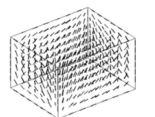
Figure 4: Unwrapped configuration in class $h_{0}$

The lower bound for the infimum energy of Theorem 3.2 is $4\pi L_{z}$. The upper bound of Theorem 5.3 can be improved in this case by explicit evaluation of the Dirichlet energy for a trial configuration, yielding

$$E_{R}^{\text{inf}}(h_{0}) <8\frac{L_{y}L_{z}}{L_{x}^{2}}F_{2}\left(1,{\textstyle\frac{1}{2}},{\textstyle\frac{1}{2}},{\textstyle\frac{1}{2}},{\textstyle\frac{1}{2}},-\frac{L_{y}^{2}}{L_{x}^{2}},-\frac{L_{z}^{2}}{L_{x}^{2}}\right)$$

$$\ \ +(x\rightarrow y\rightarrow z)+(x\rightarrow z\rightarrow y),$$ (44)

where $F_{2}(\alpha,\beta,\beta^{\prime},\gamma,\gamma^{\prime};s,t)$ is the Appell hypergeometric function [5]. For a unit cube, we get the bounds

$$12.5\lesssim E_{R}^{\text{inf}}(h_{0})\lesssim 15.3$$ (45)

We computed minimisers numerically using two methods, namely solution of the Euler-Lagrange equation (using FEMLAB, a commercial PDE solver) and gradient descent. The converged energies from both methods agree, giving approximately $14.8$. The converged unit-vector field is indistinguishable from Fig. 4 at the resolution shown, and appears to be regular away from the vertices.

The homotopy class $h_{1}$ is the next simplest among the reflection-symmetric conformal classes. There are three nonzero wrapping numbers equal to $-1$ in contiguous octants, so that ${\bf n}$ takes values in three-quarters of a hemisphere. The restriction of ${\bf n}$ to a spherical cleaved surface corresponds to the conformal map

$$f_{1}(w)=w\frac{w^{2}+s^{2}}{s^{2}w^{2}+1}.$$ (46)

Such a configuration is shown in Fig. 5. On the $xy$-faces of the prism, ${\bf n}$ executes a three-quarter turn about each vertex, corresponding to kink numbers of $\pm 1$; the kink numbers on the other faces all vanish. As the parameter $s$ approaches $1$ from below, half-turns becomes concentrated along the $y$-edges, while $f_{1}$ approaches $f_{0}$ away from the $y$-edges. The corresponding family of configurations ${\bf n}_{s}$ is weakly but not strongly continuous with respect to $s$ (an example of the fact that $h_{1}$ is not weakly closed).

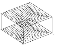
Figure 5: A configuration ${\bf n}$ in $h_{1}$, generated by the conformal map $f(w)=w(w^{2}+s^{2})/(s^{2}w^{2}+1)$ for $s=.5$. ${\bf n}$ describes a 3/4-turn about each vertex in the top and bottom face.

Both numerical methods indicate that $h_{1}$ supports a smooth local minimiser for sufficiently thin slabs ($L_{x}/L_{y},L_{x}/L_{z}\lesssim 1/10$), while for aspect ratios closer to unity, the numerical solution converges to the minimiser in $h_{0}$. Some insight into this behaviour is provided by computing the Dirichlet energy of trial configurations characterised by the one-parameter family (46), as shown in Fig. 6. For a cube (dashed curve), the energy approaches a minimum as $s$ approaches 1, corresponding to a configuration in which half-turns concentrate along the $y$-edges. For $L_{x}=20$, $L_{y}=10$, $L_{z}=1$ (solid curve), the energy has a minimum for $s$ between $0$ and $1$, corresponding to a smooth configuration. Note that concentration along the shortest ($L_{z}$)-edges (which support the minimal connection) is not compatible with the topology, as the nonzero kink numbers lie in the $xy$-faces. Analogous arguments suggest that reflection-symmetric homotopy classes with two or more nonzero kink numbers do not contain smooth minimisers (for these classes, concentration along the shortest edge is compatible with the topology). However, it is conceivable that more non-reflection-symmetric homotopy classes (for which minimal connections do not necessarily pair vertices along edges) support smooth local minimisers.

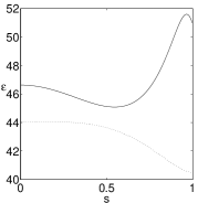
Figure 6: Scaled energy $\epsilon=E/(L_{x}L_{y}L_{z})^{1/3}$ of the conformal configuration $w(w^{2}+s^{2})/(s^{2}w^{2}+1)$. Solid curve: $L_{x}=20$, $L_{y}=10$, $L_{z}=1$. Dashed curve: $L_{x}=L_{y}=L_{z}=1$.

The last numerical example is an idealised model of the PABN device. Details are given in [12]. In fact, the model lies outside the class of problems we have considered so far; the domain is not a polyhedron, and the boundary conditions are not purely tangent. We take the PABN to consist of a rectangular post of square cross-section centred on the bottom surface of a rectangular cell of square cross-section, as in Fig. 7. In keeping with the device dimensions, the cell height is taken to be three times the cell width, and the cell width to be twice the post width. The height of the post is variable. Boundary conditions are dictated by material characteristics of the substrates. Tangent boundary conditions apply on the bottom substrate and on the post, while normal boundary conditions are appropriate for the top substrate. Periodic boundary conditions are imposed on the vertical sides of the cell, simulating a two-dimensional array of cells supporting the same nematic configuration (at a given time) and comprising a single pixel.

We consider four simple homotopy classes, in which the kink numbers are zero and the trapped areas taken to have their minimal allowed values. The orientation of ${\bf n}$ on the horizontal edges of the post are fixed, as in Fig 7(a). The classes are distinguished by the relative orientations of ${\bf n}$ on the vertical edges of the post. Up to symmetry, there are four distinct possibilities. For the tilted class $T$, the orientation on all four vertical edges is the same. The other three classes, called planar, are obtained by taking the orientation to be opposite on, respectively, one of the vertical edges (the $P_{1}$ class), two adjacent vertical edges ($P_{2}$), and two opposing vertical edges ($P_{3}$). Configurations in $T$ exihibit a large vertical component $n_{z}$ in the region around the post. In configurations in $P_{1}$ – $P_{3}$, $n_{z}$ is suppressed by the change in orientation between the vertical edges.

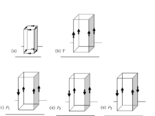
Figure 7: Edge orientations for the four PABN configurations. (a) Orientations on the horizontal edges are the same for all. (b) Tilted profile $T$. ${\bf n}$ points up on all vertical edges. (c) Planar profile $P_{1}$. ${\bf n}$ points down on a single vertical edge (d) Planar profile $P_{2}$. ${\bf n}$ points down on a pair of adjacent vertical edges (e) Planar profile $P_{3}$. ${\bf n}$ points down on a pair of opposite vertical edges.

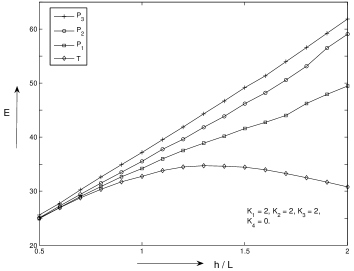
Figure 8: Energies in the PABN cell as a function of post height

Local minimisers for each of these homotopy classes were computed using FEMLAB for a range of post heights. The converged configurations appear to be smooth away from the vertices of the post. In Figure 8 we plot the converged energies of the local minimisers as a function of post height. The tilted class has the lowest energy, which is consistent with experimental observations which show that the liquid crystal always relaxes into the high-tilt state when cooled from the isotropic state [8]. The computations support the hypothesis that the bistable states of the PABN are topologically distinct.

Acknowledgments. We thank CJP Newton, our co-author on [12], for many helpful discussions and, along with A Geisow, for stimulating our interest in these problems. AM was partially supported by an EPSRC/Hewlett-Packard Industrial CASE Studentship. AM and MZ were partially supported by EPSRC grant EP/C519620/1.

References

- [1] G. Birkhoff. Tres observaciones sobre el algebra lineal. Univ. Nac. Tacumán Rev, Ser. A, (5):147–151, 1946.
- [2] H. Brezis, J.-M. Coron, and E.H. Lieb. Harmonic maps with defects. Comm. Math. Phys., 107:649–705, 1986.
- [3] P.-G. de Gennes and J. Prost. The physics of liquid crystals. Oxford University Press, 2nd edition, 1995.
- [4] F. Duzaar and G. Mingione. The p-harmonic approximation and the regularity of p-harmonic maps. Calc. Var., 20:235–256, 2004.
- [5] I.S. Gradshteyn and I.M. Ryzhik. Tables of Integrals, Series and Products. Academic Press, 1980.
- [6] R. Hardt and F.H. Lin. Stability of singularities of minimizing harmonic maps. Journal of Differential Geometry, 29:113–123, 1989.
- [7] J.C. Jones, J.R. Hughes, A. Graham, P. Brett, G.P. Bryan-Brown, and E.L. Wood. Zenithal bistable devices: Towards the electronic book with a simple LCD. In Proc IDW, pages 301–304, 2000.
- [8] S. Kitson and A. Geisow. Controllable alignment of nematic liquid crystals around microscopic posts: Stabilization of multiple states. Appl. Phys. Lett., 80:3635 – 3637, 2002.
- [9] M. Kleman and O.D. Lavrentovich. Soft Condensed Matter. Springer, 2002.
- [10] W. Magnus, A. Karras, and D. Solitar. Combinatorial group theory. Dover, 1976.
- [11] A. Majumdar. Liquid crystals and tangent unit-vector fields in polyhedral geometries. PhD thesis, University of Bristol, 2006.
- [12] A. Majumdar, C.J.P. Newton, J.M. Robbins, and M. Zyskin. Topology and bistability in liquid crystal devices. Phys. Rev. E, 75:051703 (11 pages), 2007.
- [13] A. Majumdar, J.M. Robbins, and M. Zyskin. Elastic energy of liquid crystals in convex polyhedra. J. Phys. A, 37:L573–L580, 2004. ; J. Phys. A 38 (2005) 7595-7595.
- [14] A. Majumdar, J.M. Robbins, and M. Zyskin. Lower bound for energies of harmonic tangent unit-vector fields on convex polyhedra. Lett. Math. Phys., 70:169–183, 2004.
- [15] A. Majumdar, J.M. Robbins, and M. Zyskin. 2008. in preparation.
- [16] A. Majumdar, J.M. Robbins, and M. Zyskin. Energies of -valued harmonic maps on polyhedra with tangent boundary conditions. Annales de l’Institut Henri Poincare (C) Non Linear Analysis, 25:77–103, 2008.
- [17] R. Moser. Partial regularity for harmonic maps and related problems. World Scientific, 2005.
- [18] J.M. Robbins and M. Zyskin. Classification of unit-vector fields in convex polyhedra with tangent boundary conditions. J. Phys. A, 37:10609–10623, 2004.
- [19] R. Schoen and K. Uhlenbeck. A regularity theory for harmonic maps. J. Diff. Geom., 17:307–335, 1982.
- [20] R. Schoen and K. Uhlenbeck. Boundary regularity and the Dirichlet problem for harmonic maps. J. Diff. Geom., 18:253–268, 1983.
- [21] Iain W. Stewart. The Static and Dynamic Continuum Theory of Liquid Crystals. Taylor and Francis, London, 2004.
- [22] C. Tsakonas, A.J. Davidson, C.V. Brown, and N.J. Mottram. Multistable alignment states in nematic liquid crystal filled wells. App. Phys. Lett., 90:111913 (3 pages), 2007.
- [23] E.G. Virga. Variational Theories for Liquid Crystals. Chapman and Hall, 1994.