Spitzer Quasar and ULIRG Evolution Study (QUEST). IV.
Comparison of 1-Jy Ultraluminous Infrared Galaxies with Palomar-Green Quasars

Abstract

We report the results from a comprehensive study of 74 ultraluminous infrared galaxies (ULIRGs) and 34 Palomar-Green (PG) quasars within $z\sim 0.3$ observed with the Spitzer Infrared Spectrograph (IRS). The contribution of nuclear activity to the bolometric luminosity in these systems is quantified using six independent methods that span a range in wavelength and give consistent results within $\sim$ $\pm$10$-$15% on average. This agreement suggests that deeply buried AGN invisible to Spitzer IRS but bright in the far-infrared are not common in this sample. The average derived AGN contribution in ULIRGs is $\sim$35$-$40%, ranging from $\sim 15-35$% among “cool” ($f_{25}/f_{60}\leq 0.2$) optically classified HII-like and LINER ULIRGs to $\sim$50 and $\sim$75% among warm Seyfert 2 and Seyfert 1 ULIRGs, respectively. This number exceeds $\sim$80% in PG QSOs. ULIRGs fall in one of three distinct AGN classes: (1) objects with small extinctions and large PAH equivalent widths are highly starburst-dominated; (2) systems with large extinctions and modest PAH equivalent widths have larger AGN contributions, but still tend to be starburst-dominated; and (3) ULIRGs with both small extinctions and small PAH equivalent widths host AGN that are at least as powerful as the starbursts. The AGN contributions in class 2 ULIRGs are more uncertain than in the other objects, and we cannot formally rule out the possibility that these objects represent a physically distinct type of ULIRGs. A morphological trend is seen along the sequence $(1)-(2)-(3)$, in general agreement with the standard ULIRG $-$ QSO evolution scenario and suggestive of a broad peak in extinction during the intermediate stages of merger evolution. However, the scatter in this sequence, including the presence of a significant number of AGN-dominated systems prior to coalesence and starburst-dominated but fully merged systems, implies that black hole accretion, in addition to depending on the merger phase, also has a strong chaotic/random component, as in local AGN.

1. Introduction

More than twenty years ago, Sanders et al. (1988a, 1988b) proposed the existence of an evolutionary connection between ultraluminous infrared galaxies (ULIRGs; log[$L$(IR)$/L_{\odot}$] $\geq$ 12) and quasars. Their imaging and spectrophotometric data on ten local ULIRGs were interpreted to imply that ULIRGs are dust-enshrouded quasars formed through the strong interaction or merger of two gas-rich spirals. This merging process had long been suspected to lead to the formation of an elliptical galaxy (e.g., Toomre & Toomre 1972) and subsequent numerical simulations have lent support to this idea (e.g., Barnes 1989; Kormendy & Sanders 1992; Springel et al. 2005; Bournaud et al. 2005; Naab et al. 2006). ULIRGs have been found since then to be an important population in the distant universe, a major contributor to the cosmic star formation at $z\gtrsim 1-2$ (see, e.g., reviews by Sanders & Mirabel 1996; Blain et al. 2002; Lonsdale et al. 2006). The evidence is growing that the majority of the high-z ULIRGs are fed by continuous gas accretion, and only about one third are gas-rich (“wet”) mergers (Daddi et al. 2007; Shapiro et al. 2008; Genzel et al. 2006, 2008; Förster Schreiber et al. 2006, 2009; Genel et al. 2008; Dekel & Birnboim 2008; Dekel et al. 2009). However, the fraction of ULIRGs involved in mergers appears to increase steeply at higher infrared luminosity (e.g., submillimeter-selected galaxies; Tacconi et al. 2006, 2008).

Considerable effort has been devoted in the past decade to understand ULIRGs and quasars in the local universe, where galaxy merging and its relation to starbursts and AGN can be studied in greater detail than in the distant universe. Our group is conducting a comprehensive, multiwavelength imaging and spectroscopic survey of local ULIRG and QSO mergers called QUEST – Quasar and ULIRG Evolution STudy. QUEST has already provided crucial new insights into merger morphology, kinematics, and evolution: we now know that ULIRGs are advanced mergers of gas-rich, disk galaxies sampling the Toomre merger sequence beyond the first peri-passage (Veilleux et al. 2002). The near-infrared (NIR) light distributions in many ULIRGs, particularly those with AGN-like optical and infrared characteristics, show prominent early-type morphology ($R^{1/4}$ law; Wright et al. 1990; Scoville et al. 2000; Veilleux et al. 2002, 2006). The hosts of ULIRGs lie close to the locations of intermediate-size ($\sim$ 1 – 2 $L^{*}$) spheroids in the photometric projection of the fundamental plane of ellipticals, although there is a tendency for the ULIRGs with small hosts to be brighter than normal spheroids. Excess emission from a merger-triggered burst of star formation in the ULIRG hosts may be at the origin of this difference.

NIR stellar absorption spectroscopy with the VLT and Keck has also been carried out by our group to constrain the host dynamical mass for many of these ULIRGs. The analysis of these data (Dasyra et al. 2006a, 2006b) built on the analyses of Genzel et al. (2001) and Tacconi et al. (2002) and revealed that the majority of ULIRGs are triggered by almost equal-mass major mergers of 1.5:1 average ratio, in general agreement with Veilleux et al. (2002). In Dasyra et al.  we also found that coalesced ULIRGs resemble intermediate mass ellipticals/lenticulars with moderate rotation, in their velocity dispersion distribution, their location in the fundamental plane and their distribution of the ratio of rotation/velocity dispersion [v_rot sin(i)/$\sigma$]. These results therefore suggest that ULIRGs form moderate mass ($m^{\ast}\sim 10^{11}$ M_⊙), but not giant (5 – 10 $\times$ 10¹¹ M_⊙) ellipticals. Converting the host dispersion into black hole mass with the aid of the M_BH – $\sigma_{*}$ relation (e.g., Gebhardt et al. 2000, Ferrarese & Merritt 2000) yields black hole mass estimates ranging from 10^7.0 $M_{\odot}$ to 10^8.7 $M_{\odot}$, with slightly larger values in coalesced ULIRGs than in binaries. BH masses derived from similar data on a dozen PG QSOs agree with those of coalesced ULIRGs (Dasyra et al. 2007). A recent analysis of HST/NICMOS data on several of these PG QSOs appears to support this conclusion (Veilleux et al. 2009; see also Surace et al. 2001; Guyon et al. 2006).

QUEST has also provided new quantitative information on the importance of gas flows in and out of ULIRGs. Direct evidence for powerful galaxy-scale winds has been found in most ULIRGs (e.g., Rupke et al. 2002, 2005a, 2005b, 2005c; see also Martin 2005 and Veilleux et al. 2005), and the metal underabundance and smaller yield measured in the cores of these objects (Rupke et al. 2008) point to strong merger-induced gas inflows in the recent past as predicted by numerical simulations (e.g., Barnes & Hernquist 1996; Mihos & Hernquist 1996; Iono et al. 2004; Naab et al. 2006).

The last two crucial issues addressed by QUEST are the nature of the energy production mechanism – starburst or AGN – in ULIRGs and QSOs and the importance of dust extinction along the merger sequence. Early optical and NIR spectroscopy has revealed trends of increasing AGN dominance among ULIRGs with the largest infrared luminosity, warmest 25-to-60 $\mu$m color, and latest merger phase (e.g., Veilleux et al. 2006 and references therein), but these results are potentially biased by dust obscuration. Mid-infrared (MIR) spectroscopy with the Infrared Space Observatory (ISO) (e.g., Genzel et al. 1998; Lutz et al. 1998b; Lutz et al. 1999; Rigopoulou et al. 1999; Tran et al. 2001) has provided crucial new information on the energy source in ULIRGs, less affected by the effects of dust, although the number of objects in the sample was limited by the relatively modest sensitivity of ISO.

The most recent progress in this area of research occurred with the advent of the Spitzer Space Telescope. The Infrared Spectrograph (IRS) Guaranteed-Time and General Observation (GTO and GO) programs have provided a wealth of new information on the physical properties of local ULIRGs (e.g., Armus et al. 2004, 2007; Farrah et al. 2007; Desai et al. 2007; Hao et al. 2007; Higdon et al. 2006; Imanishi et al. 2007; Lahuis et al. 2007; Spoon et al. 2007; CAo et al. 2008). In the present paper, we revisit a carefully selected subset of these data and combine them with GO-1 IRS data acquired by our QUEST program, to calculate AGN contributions to the total bolometric luminosities, quantify the issue of ULIRG evolution along the merger sequence, and to determine where, if at all, quasars fit in this picture.

Our earlier papers in this series have focussed exclusively on the QSOs. In Schweitzer et al. (2006; Paper I), we showed that starbursts are responsible for at least $\sim$30%, but likely most, of the FIR luminosity of PG QSOs. We argued in Netzer et al. (2007; Paper II) that both strong- and weak-FIR emitting sources have the same, or very similar, intrinsic AGN spectral energy distributions (SEDs). In Schweitzer et al. (2008; Paper III), we found that emission from dust in the innermost part of the narrow-line region is needed in addition to the traditional obscuring torus in order to explain the silicate emission in these QSOs. The present paper reports the results from our analysis of the continuum, emission line, and absorption line properties of 74 ULIRGs and 34 QSOs. In Section 2, we describe the sample. Next, we discuss the observational strategy of our program and the methods we used to obtain, reduce, and analyze the IRS spectra, including the archived data (Section 3, Section 4, and Section 5, respectively). The results are presented in Section 6 and tested against the evolution scenario of Sanders et al. (1988a, 1988b) in Section 7. The main results and conclusions are summarized in Section 8. Throughout this paper, we adopt $H_{0}$ = 70 km s^-1 Mpc^-1, $\Omega_{M}$ = 0.3, and $\Omega_{\Lambda}$ = 0.7.

2. Sample

The basic properties of the ULIRGs and quasars in our sample are listed individually in Table 8. For a summary of the properties of the ULIRGs by spectral types, infrared colors and luminosities, and morphology, see Table 11. The ULIRG component of our program focuses on the 1-Jy sample, a complete flux-limited sample of 118 ULIRGs selected at 60 $\mu$m from a redshift survey of the IRAS faint source catalog (Kim & Sanders 1998). All 1-Jy ULIRGs have $z<0.3$. Twenty-nine objects were observed under our own Cycle 1 medium-size program (#3187; PI Veilleux; Note that the 1-Jy ULIRG Mrk 1014 is also PG 0157+001). These objects were selected to be representative of the 1-Jy sample as a whole in terms of redshift, luminosity, and IRAS 25-to-60 $\mu$m colors. These data were supplemented by archival IRS spectra of 39 other galaxies from the 1-Jy sample, and 5 archival IRS spectra of infrared-luminous galaxies from the Revised Bright Galaxy Sample (RBGS, Sanders et al. 2003; these objects are UGC 05101, F10565+2448, F15250+3609, NGC 6240, and F17208$-$0014). Most of the archival spectra are from GTO program #105 (PI Houck), and three are from GO program #20375 (PI Armus). These spectra cover bright sources in the 1 Jy sample, while ours are deeper exposures of fainter ones. Together, they represent almost 2/3 of the 1 Jy sample. The 5 RBGS spectra represent well-studied benchmarks from the local universe. Figure 1 shows the distributions of redshifts, infrared luminosities, and 25-to-60 $\mu$m IRAS colors for the combined set of ULIRGs compared with that of the entire 1-Jy sample. We confirm that the ULIRGs in our study are representative of the range of properties of the 1-Jy sample. Optical spectral types, which are referred to extensively in this paper, are taken from Veilleux et al. 1999a and Rupke et al. 2005a for the 1 Jy sample, and Veilleux et al. 1995 for the 5 RBGS objects.

The original QUEST sample of quasars has already been discussed in detail in Papers I and II and this discussion will not be repeated here. Suffice it to say that the original QUEST sample contains 25 $z\lesssim 0.3$ quasars, including 24 Palomar-Green (PG) quasars from the Bright Quasar Sample (Schmidt & Green 1983) and another one (B2 2201+31A = 4C 31.63) with a $B$ magnitude that actually satisfies the PG QSO completeness criterion of Schmidt & Green (1983). Nine other PG QSOs (PG 0050+124 = I Zw 1, PG 0804+761, PG 1119+120 = Mrk 734, PG 1211+143 = Mrk 841, PG 1244+026 [NLS1], PG 1351+640, PG 1448+273 [NLS1], and PG 1501+106) observed under different Spitzer programs were later added to the quasar sample. Figure 2 emphasizes the fact that the quasars in our study cover the low redshift and low B-band luminosity ends of the PG QSO sample, while Figure 3 shows that the ULIRGs and quasars in our study are well matched in redshift. Finally, note that two ULIRGs, Mrk 1014 and 3C 273, are also PG QSOs; we treat them as ULIRGs for the purposes of this study.

High-quality optical and NIR images obtained from the ground and with HST are available for all ULIRGs and quasars in the present sample (e.g, Surace & Sanders 1999; Scoville et al. 2000; Surace et al. 1998, 2001; Guyon et al. 2006; Veilleux et al. 2002, 2006, 2009). In addition, high-quality optical spectra exist for all 1-Jy ULIRGs (e.g., Veilleux et al. 1999a; Farrah et al. 2005; Rupke et al. 2005a, 2005b, 2005c) and PG QSOs (Boroson & Green 1992), and a large subset of these objects also have been the targets of NIR JHK-band spectroscopy by our group over the years (e.g., Veilleux et al. 1997, 1999b; Dasyra et al. 2006a, 2006b, 2007) as well as some L-band spectroscopy (e.g., Imanishi et al. 2006a; Risaliti et al. 2006; Imanishi et al. 2008; Sani et al. 2008). These ancillary data will be used for our interpretation of the Spitzer data in Section 6 and Section 7.

3. Observations

Galaxies from our own program (#3187; PI Veilleux) were observed in the IRS modules SL, SH, and LH, using staring mode (Houck et al. 2004). Together, these modules cover observed wavelengths of $5-35$ µm. The high resolution data at observed wavelengths of $10-35$ µm (SH and LH modules, with resolution $R\sim 600$) allow sensitive measurements of important atomic and molecular emission lines.

For targeting, moderate-accuracy IRS blue peak-ups were performed on the targets themselves rather than offsetting from 2MASS stars. This peak-up method is justified given the compact MIR continua in these systems (e.g., Soifer et al. 2000; Surace et al. 2006).

For the four binary ULIRGs with nuclear separations exceeding 3″ (F01166$-$0844, F10190$+$1322, F13454$-$2956, and F21208$-$0519), a unique observation was made of each nucleus. However, in 3 of these cases (F10190$+$1322 being the exception), aperture effects due to the larger slit sizes of the long-wavelength modules allowed accurate measurements of only one of the two nuclei.

The observational setup used for the archival IRS spectra is described in detail in Armus et al. (2007) and references therein. It is essentially the same as the one we used for our own program so direct comparison between the two data sets is permissible.

Some objects in our sample have full low-resolution spectra (i.e., including both the SL and LL modules, covering $5-35$ µm). We have used only the high-resolution data for spectral line measurements (except for the [Ne VI] line, which falls in the SL module). The LL data was used primarily for checking flux calibration. However, when only SL$+$LL data was available, or when the high-resolution data was of low S/N, the full low-resolution spectrum was used in the continuum fitting.

Spitzer proposal ID numbers and exposure times for each IRS module are listed for all galaxies in Table 2.

4. Data Reduction

For the majority of QUEST sources, we started with BCD data processed by version S12.0 of the IRS pipeline. For the non-QUEST 1 Jy ULIRGs that were reduced at a later date, data from pipelines S12, S13, or S15 were used. Comparisons among these pipelines show only minor differences that do not impact our measurements.

The data were first corrected for rogue pixels using an automatic search-and-interpolate algorithm (which was supplemented by visual examination). For the SL module, background light was then subtracted by differencing the two nod positions. For the SL and LL modules, the data was extracted prior to coadding. For SH and LH, we coadded exposures for a given nod position prior to extraction.

The one-dimensional spectra were extracted using the Spectroscopic Modeling Analysis and Reduction Tool (SMART; Higdon et al. 2004). The extraction apertures were tapered with wavelength to match the point-spread function for SL and LL data and encompassed the entire slit for SH and LH data. The correction/extraction process was iterated until we were assured that the majority of hot pixels had been removed.

For SL, we combined the two one-dimensional nod spectra for the orders SL1 and SL2 separately and then stitched the orders by trimming a few pixels from one or the other order. (We discarded SL3 because of flux discrepancies.) For SH and LH, we combined the two nods and then stitched the orders together by applying multiplicative offsets for each order that were linear in flux density vs. wavelength (effectively removing a tilt artifact from certain orders where necessary).

We subtracted zodiacal light from the high-resolution data using a blackbody fit to the Spitzer Planning Observations Tool (SPOT) zodiacal estimates at 10, 20, and 35$\micron$.

Finally, we matched modules in flux to form complete $5-35$ µm spectra. Because ULIRGs are compact mid-IR sources, different modules in general agree well in flux at wavelengths where they overlap. Where there was disagreement, we used available low-resolution spectra (SL $+$ LL) to improve the zodiacal subtraction, since these spectra were sky-subtracted using simultaneous sky observations. Where this was not possible, we used small additive offsets.

To check the flux calibration, we computed synthetic IRAS flux densities at 12 and 25 µm using the Spitzer data by averaging the flux densities over the IRAS bandpasses. At 25 µm, the agreement with IRAS is excellent (Figure 4). The median IRAS-to-Spitzer flux density ratio is 1.04, with a standard deviation of 0.3. At 12 µm, most of the IRAS fluxes are upper limits, but the agreement is still decent ($f_{12}^{IRAS}/f_{12}^{Spitzer}\sim 1.25$ on average for sources with $f_{12}>0.1$ Jy). The cause of the small discrepancy at 12µm is unclear, but may result from Eddington-Malmquist bias.

In this paper, we adopt the Spitzer-derived 12 and 25 $\mu$m fluxes to avoid the use of IRAS upper limits, a particularly severe problem for the LINER and HII-like ULIRGs of our sample.

5. Data Analysis

5.1. Emission Lines

In Tables 3 and 4, we list atomic and molecular emission-line fluxes measured from our spectra. Measurements were made with the IDEA tool in SMART; we fitted Gaussian profiles atop a linear continuum. Upper limits were determined by assuming an unresolved line. The available resolution allowed us to decompose close line blends, including the important [Ne V] $14.32$ µm / [Cl II] $14.36$ µm and [O IV] $25.89$ µm / [Fe II] $25.99$ µm blends.

5.2. Continuum and Dust Features

A vitally important task was to properly model the sum of the blackbody continuum emission, which is punctuated by deep extinction and absorption features, and the full-featured small dust grain continuum. The primary goal of this modelling was to accurately extract the fluxes of absorbed PAH features, but we also gained useful information about the continuum. Because we are not concerned with detailed physics, we have chosen a simple, but robust and empirically-motivated, method.

Before fitting, we measured narrow-band flux densities (of width 3.3% of the central wavelength) at regularly-spaced intervals across the continuum, avoiding deep absorption features. These are listed in Table 5.

To fit the MIR spectra, we used the IDL package developed to model the blackbody and silicate emission of QUEST quasars (Paper III). We refer to this paper for the basic fitting details. Here we describe some unique features necessary for fitting the spectra of PAH-strong and sometimes deeply-absorbed ULIRGs. Typical fits are shown in Figure 5.

1. A modified version of the Chiar & Tielens (2006) Galactic Center extinction curve was used. To the basic extinction profile, we added extinction from the water ice plus hydrocarbon feature at $5.7-7.8$ µm. The profile is taken from observations of F00183$-$7111 (Spoon et al. 2004). In place of the broad silicate features at 9.7 and 18 µm  we substituted features that were empirically derived from the deeply absorbed and almost completely PAH-free ULIRG, F08572$+$3915. The silicate profile of this galaxy provides a universally good fit to the ULIRGs in our sample. However, using the original Chiar & Tielens silicate profile, or one from a less deeply-absorbed system, yields poor fits at high optical depths in a number of deeply absorbed systems. The strengths of the water ice $+$ hydrocarbon feature and silicate absorption $+$ overall extinction curve were allowed to vary independently. Foreground and mixed dust screens were both tried, and we found that foreground screens fit better.

2. We fit three blackbodies to almost all spectra. These blackbodies represent a convenient parameterization of the MIR continuum. Due to the absence of wavelengths probing the hottest and coldest dust, the temperatures of these blackbodies do not represent actual dust components. Nonetheless, their values provide useful guidance in understanding the shape of the continuum. For most sources, three is the minimum number of blackbodies that produce an acceptable fit. However, the use of two or four blackbodies significantly improved the fit in six cases.

3. The temperatures, water ice $+$ hydrocarbon absorption, and extinctions of the blackbodies were in general allowed to freely vary (see results in Table 6). However, in some cases the water ice plus hydrocarbon absorption and/or the extinction had to be fixed to zero in a particular component, when it was apparent that the fitted value was unphysical. In a handful of cases, the temperature of the hottest component was also poorly constrained by the fit. Experimentation and by-eye examination suggests that these unconstrained temperatures are not much larger than 1000 K, to which we fixed them. The actual temperatures are probably in the range $\sim 700-2000$ K.

4. PAH emission was modeled using the average MIR spectra derived from the SINGS program galaxies (Smith et al. 2007). Pure PAH templates were created by running the PAHFIT program (Smith et al. 2007) to extract the PAH emission features from the four average SINGS spectra (including the 17 $\mu$m emission band; van Kerckhoven et al. 2000; Peeters et al. 2004). The PAH model underlying PAHFIT is a series of Drude profiles; the 6.2 and 7.7 µm features, which we discuss in §6.3, consist of 1 and 3 Drude components, respectively. Note that the templates output by PAHFIT consist only of PAH emission, without an associated continuum from star formation regions; this continuum is fit by the blackbodies mentioned above. We chose two of these templates (from Smith’s 3rd and 4th average SINGS spectra) that provided the largest range in the ratio of the 7.7 µm and 11.2 µm PAH features. The overall strengths of these two pure PAH templates were allowed to vary in the fit.

   The fit results, listed in Table 7, were not sensitive to the choice of pure PAH template. Only a small range ($\sim$ 0.13 dex) in PAH 6.2/7.7 µm and 7.7/11.2 µm ratios was allowed by the two PAH templates and most galaxies are dominated by one or the other template. We found that using templates produced from SINGS spectra of galaxies with very low values of the 7.7/11.2 µm ratio (J. D. Smith 2007, pvt. comm.) yielded poor fits. Thus, the strong suppression of the 6.2 or 7.7 µm complex observed in galaxies that host low-luminosity AGN (Sturm et al. 2006; Smith et al. 2007) and in some star-forming regions (Hony et al. 2001) does not occur in ULIRGs.

   We found that allowing PAH extinction below the level of $A_{V}\sim 10$ did not significantly affect the fits (i.e., the results were basically indistinguishable from the $A_{V}=0$ case). We thus left the PAHs unextincted in most cases. Adding larger amounts of extinction had the effect of raising the 7.7/11.2 µm ratio and almost always made the fits worse. However, in four cases we allowed the PAH features to be extincted at or above the $A_{V}\sim 10$ level because the fit was significantly improved. These four cases are as follows, with PAH extinction in parentheses (two values indicate two fitted components): F00397$-$1312 ($A_{V}=44$), F01494$-$1845 ($A_{V}=$ 10/14), F20414$-$1651 ($A_{V}=$ 0/22), F21208$-$0519:N ($A_{V}=11$). These values correspond well with the effective continuum extinction (Section 6.2) in these sources: $A_{V}\sim$ 50, 18, 18, and 15, respectively. We discuss PAH extinction further in Section 6.3.

5. For four galaxies (Mrk 1014, F07598$+$6508, 3C 273, and F21219$-$1757) we included silicate emission components, as described in Paper III.

6. Due to the absence of pipeline error spectra, the mixing of data over a significant flux range, and the different dispersion among different IRS modules, careful weighting had to be performed during the fits (see Paper III for details). We tried three methods: (1) weighting based on the actual fluxes; (2) weighting based on a power-law fit to the fluxes; and (3) an average of the two. In almost all cases, the third method produced the best fits. However, in isolated cases we used one of the other weighting schemes if it was clearly superior.

Along with the ULIRGs in our sample, we also did three-blackbody fits, with both silicate and PAH emission included, to the three average PG QSO spectra from Paper II. These spectra were divided by FIR strength into FIR-strong QSOs, FIR-weak, and FIR-undetected. These new fits differ from the fits in Papers I and III in that Paper I fit only the PAHs using simple Lorentzian fits to a few individual features, while Paper III presented more formal fits but did not include PAH emission. Here we include all components, and make sure that the PAH fits of the QSOs are done using the same procedures applied here to the ULIRGs.

6. Results

The IRS spectra of all ULIRGs in the current study are presented in Figure 6, with archival photometry overplotted: $J$, $H$, and $K$, and flux densities at 12, 25, 60, and 100 µm. The NIR photometry is from 2MASS and Sanders et al. (1988a). The far-infrared photometry is mostly from the IRAS Faint Source Catalog, but also includes some data from Sanders et al. (2003) and a few $ISO$ 12 µm points from Klaas et al. (2001). The IRS spectra of the QSOs were presented in Paper II, so they are not shown here again. The basic results from our analysis are listed in Tables $\ref{tab:eml1}-\ref{tab:pahs}$.

In this section, we first describe the results from our analysis of the broadband continuum emission in Section 6.1 before discussing the absorption and emission-line features in Section 6.2 and Sections $6.3-6.6$, respectively.

6.1. Broadband Continuum Emission

6.1.1 Average Spectra

We divided the sample into various categories, and produced average spectra by normalizing individual spectra to the same rest-frame, 15 µm flux density.

First, we show average spectra of “cool” ($f_{25}/f_{60}<0.1$) ULIRGs, “warm” ($f_{25}/f_{60}\geq 0.1$) ULIRGs, and all PG QSOs (Figure 7). The average spectrum of cool ULIRGs shows a steep 5-30 $\mu$m SED with strong PAH features, H₂ lines, and low-ionization fine structure lines typical of starburst-dominated systems, while PG QSOs have a shallow 5-30 $\mu$m SED with silicate features in emission and relatively strong high-ionization lines and weak PAH features typical of AGN-dominated systems. The properties of the average spectrum of warm ULIRGs are intermediate between those of cool ULIRGs and PG QSOs.

A similar exercise is carried out using the infrared luminosity: log[$L$(IR)$/L_{\odot}$] $<$ 12.3 and $\geq$ 12.3 (this threshold was selected to get roughly equal number of objects in each luminosity bin). Figure 8 shows that the contrast between low- and high-luminosity ULIRGs is nowhere near as large as between cool and warm ULIRGs. High-luminosity ULIRGs tend to be slightly warmer than low-luminosity ULIRGs so the differences we see in Figure 8 are readily explained by the correlation between Spitzer spectral characteristics and $f_{25}/f_{60}$ discussed in the previous paragraph.

In Figure 9, we divide the 1-Jy ULIRGs according to their optical spectral type. The overall 5-30 $\mu$m SED clearly steepens and the silicate absorption feature and H₂ and low-ionization fine structure emission lines clearly become stronger as one goes from the QSOs, to the Seyfert 1s, the Seyfert 2s, and finally to the LINER and H II-like ULIRGs. The averaged spectra of these last two classes of ULIRGs are hardly distinguishable from each other with the possible exception of the silicate absorption through, where we are S/N-limited (this is consistent with the ISO-based results of Lutz et al. 1999).

Finally, in Figures 10 and 11, we divide the ULIRG sample based on the equivalent width of the PAH 7.7 $\mu$m feature and the effective optical depth of the silicate absorption trough, and compare the results once again to the average spectrum of PG quasars. The strength of the PAH feature and effective optical depth of the silicate feature are derived from the SED decomposition described in Section 6.2 and Section 6.3. Strong absorption features of water ice + hydrocarbons (5.7-7.8 $\mu$m), silicate (8.5 – 12 $\mu$m), C₂H₂ 13.7 $\mu$m, and HCN 14 $\mu$m are detected in the absorption-dominated ULIRGs, similar in depth to the features seen in the heavily absorbed spectra of NGC 4418 and other galaxies including some ULIRGs (e.g., Spoon et al. 2001, 2002, 2004, 2006). Silicate absorption is visible in both PAH-dominated and PAH-weak systems. Similarly, PAH emission is detected regardless of the depth of the silicate absorption feature. As we discuss quantitatively in Section 6.3, Section 7.1, and Section 7.3, this lack of a clear trend between PAH strength and silicate absorption is largely due to the strong-AGN ULIRGs, which have weak PAHs and weak silicate absorption (see also Desai et al. 2007 and Spoon et al. 2007).

6.1.2 Continuum Diagnostics

In Figure 12, we compare the continuum flux ratios $f_{15}/f_{6}$, $f_{30}/f_{6}$, $f_{30}/f_{15}$, and $f_{25}/f_{60}$ of all ULIRGs and quasars in the sample. The “reddening” of the SED as one goes from the QSOs to the ULIRGs is evident in all panels of this figure. The best segregation by optical spectral type is seen when using $f_{25}/f_{60}$ and $f_{30}/f_{15}$. QSOs, Seyfert 1 ULIRGs, Seyfert 2 ULIRGs, and H II-like + LINER ULIRGs form a sequence of increasing 60-to-25 and 30-to-15 $\mu$m flux ratios, the H II-like ULIRGs being indistinguishable from the LINER ULIRGs. Interestingly, the optically-selected starbursts observed with ISO (Verma et al. 2003) have 25-to-60 $\mu$m and 30-to-15 $\mu$m flux ratios (Brandl et al. 2006) that are intermediate between those of H II-like/LINER ULIRGs and Seyfert 2 ULIRGs. We return to the $f_{30}/f_{15}$ ratio in Section 6.1.3 and in Section 7.1, where we discuss MIR spectral classification.

Figure 13 shows that PG QSOs and optically classified Seyfert 1, Seyfert 2, and LINER + H II-like ULIRGs progressively have weaker MIR emission relative to their FIR emission (see also Figure 7 in Paper I). The solid line represents $L$(MIR) $=L$(FIR). QSOs are well fit, on average, by the dotted line above it: $L$(MIR) $\approx 2L$(FIR). This line traces AGN-dominated systems and may be used in principle to estimate the AGN contribution to the ULIRG power. We return to this point in Section 6.1.3 and Section 7.1 of this paper. Here we simply note that the extrapolation of this line to higher MIR luminosities is a good fit to the measurements of some, but not all, Seyfert 1 ULIRGs. These latter objects are more MIR-luminous than QSOs but they have only slightly cooler SEDs than QSOs (e.g., Figures 9 and 12).

6.1.3 Results from SED Decomposition

The results from the SED decomposition analysis described in Section 5.2 are presented in Figures $\ref{fig:bbtemp}-\ref{fig:mirfir_v}$. Figure 14 shows the distributions of temperatures for the cold, warm, and hot blackbody components used in the fits. Note that, as mentioned in Section 5.2, the temperatures of hot components with $T\gtrsim 1000$ K are not well constrained in the fits. However, it is clear that Seyfert ULIRGs, particularly Seyfert 1 ULIRGs, show a tendency to have a warmer hot component than H II-like and LINER ULIRGs. This separation is not seen in the warm and cold components.

Figure 15 presents the distributions of observed monochromatic 8-, 15-, and 30-$\mu$m blackbody to total infrared luminosity ratios for all ULIRGs in the sample according to their optical spectral types. These blackbody luminosities represent the sum of all blackbody components fitted to the IRS spectra of these objects, uncorrected for extinction. K-S and Kuiper tests on these figures confirm the stronger MIR (8 and 15 $\mu$m but not 30 $\mu$m) continuum emission in Seyfert ULIRGs, particularly Seyfert 1s, than in H II-like or LINER ULIRGs. A similar result is found in Figure 16$a$, where the 5.4 - 25 $\mu$m “pure” (PAH-free and silicate-free) blackbody emission is compared to the FIR emission. This ratio is very strongly correlated with $f_{30}/f_{15}$ (Figure 16$d$). Table 5 lists for each ULIRG the observed PAH- and silicate-free 5 – 25 $\mu$m luminosities as a (logarithmic) fraction of the FIR luminosity.

One can safely assume that the continuum emission from the atmospheres of the young stars in ULIRGs, and the very hot (10³ K) small grain NIR dust emission component inferred in ISOPHOT spectra of normal galaxies (Lu et al. 2003) and presumed to also exist in these objects, do not contribute significantly to the observed continuum above $\sim$ 5 $\mu$m. Consequently, the results in Figures $\ref{fig:bbtemp}-\ref{fig:mirfir_v}$ most likely reflect an elevated AGN contribution to the MIR emission of Seyfert 1 and 2 ULIRGs relative to that of H II-like or LINER ULIRGs. This is discussed more quantitatively in Section 7.1.

6.2. Absorption Features

Table 6 lists the effective 9.7 $\mu$m silicate optical depth, $\tau^{\rm eff}_{9.7}$, defined as

$$I^{\rm eff}{\rm exp}(-\tau^{\rm eff}_{9.7})=\sum I_{i}{\rm exp}[-\tau^{i}_{9.7}],$$ (1)

where $I_{\rm eff}=\sum I_{i}$ and the sum is over the blackbody components $i$. Note that the silicate feature is in emission in four Seyfert 1 ULIRGs (Mrk 1014, F07598$+$6508, 3C 273, and 21219$-$1757) and all QSOs (Paper III). Also note that our fits were kept simple and neglected possible variations in the 18/10 $\mu$m absorption ratios in ULIRGs, so we cannot constrain the geometry of the dust distribution in these objects in detail (e.g., Sirocky et al. 2008; Li et al. 2008). For the same reason, we do not attempt to constrain the fraction of silicate absorption that is from crystalline silicates rather than amorphous silicates (e.g., Spoon et al. 2006). Finally, it is important to point out that the effective silicate optical depth discussed here is a true optical depth, defined with respect to the unextincted blackbody flux level derived from our fits. It is therefore different from those published in earlier studies (e.g., Brandl et al. 2006; Spoon et al. 2007; Armus et al. 2007; Imanishi et al. 2007), where the depth of this feature is measured empirically with respect to the observed (extincted) continuum. It would be the same if the continuum and silicates were equally extincted but unfortunately that is not generally the case. A comparison between our measurements and those published in Armus et al. (10 objects) indicate that $\tau^{\rm eff}_{9.7}\sim(2.5\pm 0.8)\tau_{9.7}({\rm Armus})$ with a median ratio of 2.8.

Figure 17 shows the distribution of $\tau^{\rm eff}_{9.7}$ vs. the optical spectral types of ULIRGs. The broad distribution of silicate strength in ULIRGs is well known from previous studies (e.g., Hao et al. 2007; Spoon et al. 2007). K-S and Kuiper tests indicate that LINER and H II-like ULIRGs have significantly larger $\tau^{\rm eff}_{9.7}$ than Seyfert ULIRGs on average, in general agreement with Spoon et al. (2007) and Sirocky et al. (2008). H II-like ULIRGs are statistically indistinguishable from LINER ULIRGs and the same is true between Seyfert 1 and Seyfert 2 ULIRGs. Combining these results with those in Section 6.1, we find that all of the Seyfert 1 ULIRGs and most of the Seyfert 2 ULIRGs cluster in the lower-left portion of the $\tau^{\rm eff}_{9.7}$ vs. $L$(8 $\mu$m)/$L$(IR), $L$(15 $\mu$m)/$L$(IR), $f_{30}/f_{6}$, and $f_{30}/f_{15}$ diagrams (Figure 18). No clear trend is seen between $\tau^{\rm eff}_{9.7}$ and $f_{30}/f_{15}$ among HII-like and LINER ULIRGs, contrary to the optically-selected starburst galaxies of Brandl et al. (2006), where objects with strong silicate absorption tend to have a steeper MIR continuum.

Also listed in Table 6 are the equivalent widths of the sum of the H₂0 ice (5.7-7.8 $\mu$m) and aliphatic hydrocarbons (6.85 + 7.25 $\mu$m) features, and individual equivalent widths for C₂H₂ 13.7 $\mu$m and HCN 14 $\mu$m. [The HCO⁺ 12.1 $\mu$m and HNC 21.7 $\mu$m features, whose millimetric transitions are important diagnostics of radiative pumping and possibly the presence of AGN (e.g., Imanishi et al. 2006b; Guélin et al. 2007), were not detected in any individual object. Upper limits of 5 $\times$ 10^-5 $\mu$m and 2 $\times$ 10^-3 $\mu$m were measured for the equivalent widths of HCO⁺ 12.1 $\mu$m and HNC 21.7 $\mu$m, respectively, in the average spectrum of ULIRGs with $\tau^{\rm eff}_{9.7}$ $>$ 3.86, the median $\tau^{\rm eff}_{9.7}$]. The equivalent widths of C₂H₂ and HCN were measured directly, using SMART, only in objects with obvious detections (26 and 20 objects, respectively, or 35% and 27% of all ULIRGs). In contrast, the equivalent width of the H₂0 ice + hydrocarbons feature was derived from the SED fit of each object. This equivalent width is calculated with respect to the blackbody continuum only (+ silicate continuum in four Seyfert 1 ULIRGs) i.e., PAH emission is not counted as continuum. Upper limits were set as follows. Each spectrum was inspected visually to determine whether or not the H₂O absorption fit was robust. For those judged questionable, the measured equivalent width was set as an upper limit. For those objects with no H₂O absorption (often because we fixed it that way) and that have a significant PAH contribution (which turn out to be HII galaxies, LINERs, or Seyfert 2s), EW(H₂O + HC) was assigned a limit of $<$ 0.1 $\mu$m. This is obviously uncertain, but implies a somewhat reasonable 5% sensitivity to absorption if the PAH contributes half the emission at these wavelengths. For the Seyfert 1s with limits only, the upper limit was set equal to that of the lowest Seyfert 1 measurement. Firm measurements exist for 46 objects (62% of all ULIRGs) and upper limits on all the others.

Interestingly, objects with the strongest C₂H₂ 13.7 $\mu$m and HCN 14 $\mu$m absorption features are not necessarily those with the strongest silicate and H₂O ice features. Indeed, Figure 19 shows that the equivalent widths of H₂O ice + hydrocarbons, C₂H₂, and HCN correlate only loosely with $\tau^{\rm eff}_{9.7}$ and between each other. This implies significant variations in composition of the dense absorbing material from one ULIRG to the next. The strongest correlation is found between C₂H₂ and HCN, which a posteriori is not surprising since both features are believed to be tracers of high-density ($>$ 10⁸ cm^-3), high-temperature chemistry (e.g., in Young Stellar Objects; Lahuis & van Dishoeck 2000; Lahuis et al. 2006, 2007).

6.3. PAHs

The PAH 6.2 and 7.7 $\mu$m equivalent widths and the total PAH to infrared and FIR luminosity ratios are listed in Table 7. The PAH luminosities are taken from our fits, and are corrected for extinction in the four sources with fitted PAH extinction (see Section 5.2 for more details). The equivalent widths are computed by dividing the PAH luminosity by the observed (extincted) continuum fluxes at 6.22 and 7.9µm. Without proper fits, the PAH 7.7$\mu$m equivalent width measurements are subject to errors in the silicate 9.7$\mu$m absorption correction. However, our fits to the entire 5-30$\mu$m IRS spectra take this effect into account in a robust manner. In what follows, we use the 7.7µm feature exclusively, though the 6.2µm feature gives identical results.

The results of our fits (Section 5.2) suggest that the detected PAHs in our sources are lightly extincted ($A_{V}<10$). This means that the extinction towards the observable PAH-emitting regions in ULIRGs is small compared to the sometimes heavily extincted blackbody-emitting regions. This is consistent with the detection of spatially extended PAH emission in compact U/LIRGs by Soifer et al. (2002).

That said, we cannot rule out heavily extincted PAHs in the cores of ULIRGs. We can set limits on the contribution of such heavily extincted components to the total, unextincted PAH emission. First we assume that any heavily obscured PAH emission is extincted to the same degree as the continuum. Then, for the median $\tau_{9.7}^{eff}$ in our sample (3.9), any heavily obscured PAH emission must constitute less than about a third of the total unextincted PAH emission for it to not significantly alter the fit. This obscured component could rise to half of the total unextincted emission if $\tau_{9.7}^{eff}$ was about twice the median ($6-7$). The four sources where PAH extinction is detected (Section 5.2) may be cases where obscured PAH emission starts to dominate.

Both PAH (e.g., Förster-Schreiber et al. 2004; Peeters et al. 2004; Calzetti et al. 2007) and FIR emission (e.g., Kennicutt 1998) are tracers of star formation in quiescent and actively star forming galaxies. We also argue in Papers I and II that PAH and FIR emission in PG QSOs are produced by star formation. We find a fairly tight distribution of $L$(PAH)/$L$(FIR) in ULIRGs (Figure 20$a$ and $b$), consistent with previous studies (Peeters et al. 2004) as well as the notion that both trace star formation. [$L$(PAH) is the total PAH flux in the $5-30$µm range.] K-S and Kuiper tests indicate no significant trend with optical spectral type. The mean and standard deviation are log $L$(PAH)/$L$(FIR) $\simeq-1.71\pm 0.3$. The same conclusions apply if $L$(IR) is substituted for $L$(FIR), and we measure log $L$(PAH)/$L$(IR) $\simeq-1.96\pm 0.3$. If the 7.7µm PAH luminosity is substituted for the total luminosity, these PAH ratios are lower by 0.4 dex. Thus, our results are consistent with $L$(PAH, 7.7µm)/$L$(FIR) for PG QSOs ($-2.0\pm 0.3$; Paper I).

However, we do find that galaxies with stronger than average silicate absorption have smaller $L$(PAH)/$L$(FIR) ratios by a factor of 2 than galaxies with weaker than average absorption, as verified with K-S and Kuiper tests (Figure 20$c$). In fact, the PAH-to-FIR ratio anticorrelates with effective silicate optical depth, such that larger extinction corresponds to smaller $L$(PAH)/$L$(FIR) (Figure 20$d$). This effect is most pronounced in the HII and LINER ULIRGs. As we note above, $\sim$ half of the intrinsic PAH emission may be completely buried in the most heavily obscured sources. A factor-of-two correction could close at least some of the discrepancy between PAH-to-FIR ratios in heavily obscured and lightly obscured ULIRGs, and further tighten the distribution of $L$(PAH)/$L$(FIR). However, we argue below that the differences we observe are more likely due to a real suppression of PAH emission.

In Figure 21$a$, we show the distribution of 7.7µm equivalent widths, which is quite broad and shows significant optical spectral type dependence. Seyfert 1 ULIRGs have much smaller PAH equivalent widths on average than H II ULIRGs (–0.78 vs 0.13), while the PAH equivalent widths of Seyfert 2 (–0.29) and LINER (–0.05) ULIRGs fall in between these values, confirming earlier ISO results (e.g., Genzel et al. 1998; Lutz et al. 1999) as well as recent Spitzer results (e.g., Desai et al. 2007; Spoon et al. 2007). PG QSOs overlap with Seyferts.

A weak luminosity dependence is also present. ULIRGs with log[$L$(IR)$/L_{\odot}$] $\geq$ 12.4 have slightly smaller 7.7µm PAH equivalent widths than lower luminosity objects (–0.36 $\pm$ 0.09 vs. 0.04 $\pm$ 0.08; Figure 21$b$), in agreement with earlier ISO results (e.g., Lutz et al. 1998b; Tran et al. 2001). The PAH equivalent widths of PG QSOs are similar to those of Seyfert 1 ULIRGs, but they do not follow the trend with infrared luminosity of the ULIRGs (this is not surprising since PG QSOs were not selected through infrared methods like the ULIRGs). The slight IR luminosity dependence of EW(PAH) among ULIRGs coincides with the excess of Seyfert 1 ULIRGs (7 out of 9) and deficit of HII ULIRGs (2 out of 18) in the high-luminosity bin of our sample. In other words, it parallels the well-known infrared luminosity dependence of the optical spectral types of ULIRGs (Veilleux et al. 1995, 1999a).

Given the trend with optical spectral type, it is not surprising to find that ULIRGs with warmer quasar-like MIR continua exhibit smaller PAH equivalent widths than cooler systems (Figure 21$c$). The $f_{30}/f_{15}$ ratio is particularly efficient at separating objects, including PG QSOs, according to their PAH equivalent widths. Arguably it is even better at it than the optical spectra type, since there is a correlation between $f_{30}/f_{15}$ and EW(PAH) among galaxies of a given spectral type. Our results also indicate that $f_{30}/f_{15}$ is a better proxy for EW(PAH) than $f_{30}/f_{6}$ and even $f_{15}/f_{6}$, the continuum color diagnostic used by Laurent et al. (2000). We return to this point in Section 7.1.

As with the PAH-to-FIR ratios (Figure 21$d$), the 7.7µm equivalent width correlates strongly with extinction in HII/LINER ULIRGs (Figure 21$d$). What is the origin of these dependences? For the PAH-to-FIR ratio, we cannot rule out extinction effects. We can for EW(PAH), as long as the continuum and any unobserved, heavily obscured PAHs are extincted to roughly the same degree. The equivalent width is, however, affected by a strongly varying amount of warm continuum. We observe a broad distribution of 8µm-to-IR ratios (Figure 15$a$), suggesting that the 8µm continuum plays an important role in regulating EW(PAH). The anticorrelation of both PAH-to-FIR ratio and EW(PAH) with extinction also points to the presence of PAH suppression at high extinction / low EW(PAH). This supression may be due to effects of high density in the cores of ULIRGs, or to destruction of PAHs in the harsh radiation field of AGN (whose importance increases with increasing optical depth in HII/LINER ULIRGs; §7.3). In our recipe for computing AGN contribution from EW(PAH), we assume that (a) PAH emission is due to star formtion and that (b) an AGN causes both an increase in the 8µm continuum and PAH suppression (§7.1).

A qualitatively similar result was found by Desai et al. (2007) and Spoon et al. (2007) using large samples of starbursts, AGN, and ULIRGs (some of these are also part of our sample). The HII and LINER ULIRGs in our sample populate a diagonal sequence joining the highly absorbed, weak-PAH ULIRGs with the unabsorbed, PAH-dominated systems; this sequence coincides with the “diagonal branch” of Spoon et al. On the other hand, all Seyfert 1 ULIRGs and many, but not all, Seyfert 2 ULIRGs in our sample have both weak silicate absorption and weak PAHs; they populate what Spoon et al. call the “horizontal branch”. The existence of these two branches may reflect true intrinsic differences in the power source and/or nuclear dust distribution between galaxies on the two branches (e.g., Levenson et al. 2007; Spoon et al. 2007; Sirocky et al. 2008). We return to this point in Section 7.1 and Section 7.3.

6.4. Fine Structure Lines

In this section we use the strengths of the fine structure lines to constrain the properties of the warm ionized gas near the central energy source of our sample galaxies. We first discuss the low-excitation features that are commonly detected in star-forming galaxies before discussing the high-excitation lines, direct probes of the AGN phenomenon.

Figure 22$a$ compares the luminosity of the [Ne II] 12.8 $\mu$m line in the ULIRGs and QSOs of our sample with the FIR luminosity. The average and median values of the [Ne II]/FIR luminosity ratios are remarkably similar regardless of the optical spectral type, including the Seyfert 1 ULIRGs and the QSOs: log $L$([Ne II])/$L$(FIR) = –3.35 $\pm$ 0.10. The similarity of this ratio for ULIRGs and QSOs was first pointed out in Paper I, where this result in combination with the similar PAH-to-FIR luminosity ratio (§6.3) was used to argue that the bulk of the FIR luminosity in QSOs is produced via obscured star formation rather than the AGN. Not surprisingly, the less obscured optically-selected ISO starbursts (Verma et al. 2003) and Seyfert galaxies (Sturm et al. 2002) plotted in Figure 22$a$ have noticeably larger [Ne II]/FIR ratios (by a factor of $\sim$ 2 and 4, respectively).

The ([Ne III] 15.5 $\mu$m)/([Ne II] 12.8 $\mu$m) line ratio is commonly used to diagnose the excitation properties of star-forming galaxies (e.g., Thornley et al. 2000; Verma et al. 2003; Brandl et al. 2006). Since the ionization potentials needed to produce Ne⁺ and Ne⁺⁺ are 21.6 and 41.0 eV, respectively, the [Ne III]/[Ne II] ratio is sensitive to the hardness of the ionizing radiation and therefore to the (effective temperature of the) most massive stars in a starburst or to the presence of an AGN, if applicable. Figure 23 shows this ratio as a function of the infrared and FIR luminosities and the MIR continuum colors, $f_{25}/f_{60}$ and $f_{30}/f_{15}$. No obvious trend with the F/IR luminosities is seen among ULIRGs. However, a clear dependence is seen with optical spectral type and MIR continuum colors, confirming earlier studies (e.g., Dale et al. 2006; Farrah et al. 2007). Larger [Ne III]/[Ne II] ratios go hand-in-hand with warmer MIR continuum. QSOs have larger [Ne III]/[Ne II] ratios on average than Seyfert ULIRGs, and Seyfert ULIRGs have larger ratios on average than HII-like and LINER ULIRGs. K-S and Kuiper tests indicate that the [Ne III]/[Ne II] ratios of LINER ULIRGs are statistically indistinguishable from those of HII-like ULIRGs, and the same statement also applies when comparing Seyfert 1 ULIRGs with Seyfert 2 ULIRGs. The two Seyfert 1 ULIRGs with [Ne III] upper limits are F07598+6508 and F13218+0552. Both of them have unusually small optical narrow-line [OIII] $\lambda$5007/H$\beta$ ratios, consistent with low-luminosity high-excitation regions (e.g., Kim et al. 1998). The dependence of [Ne III]/[Ne II] on spectral type and MIR colors induces a slight trend between this ratio and EW(PAH 7.7) (Figure 23$e$). No obvious trend between [Ne III]/[Ne II] and EW(PAH 7.7) is seen within HII-like and LINER ULIRGs, a result that is consistent with that found for optically-selected starburst galaxies (Brandl et al. 2006). Given the relatively high metallicity of ULIRGs (Section 6.6 in this paper and Rupke et al. 2008), the large [Ne III]/[Ne II] ratios seen in Seyfert ULIRGs cannot be explained by star formation alone as in the case of low-metallicity dwarf galaxies.

Other low ionization fine structure lines such as [Fe II] 25.99 $\mu$m, [S III] 33.48 $\mu$m, and [Si II] 34.82 $\mu$m have been found to be useful diagnostics of activity in galactic nuclei (e.g., Lutz et al. 2003; Sturm et al. 2005; Dale et al. 2006). Unfortunately, these lines are often redshifted out of the wavelength range of our data so they cannot be used for any kind of statistical analysis. We do not discuss these lines any further in this paper.

The ionizing spectra of all but the hottest O stars cut off near the He II edge (54.4 eV), so the detection of [O IV] 25.9 $\mu$m from three-times ionized oxygen with ionization energy $\chi$ $\sim$ 55 eV is potentially a good indicator of AGN activity. This line is detected in 30/34 QSOs, 3/9 Seyfert 1 ULIRGs, 8/13 Seyfert 2 ULIRGs, 6/28 LINER ULIRGs, and only one of the 18 HII-like ULIRGs (F21208$-$0519:N) with high-resolution spectra. In Figure 22$b$, we plot the (upper limits on the) [O IV] 25.9 $\mu$m luminosity versus the FIR luminosity of ULIRGs and QSOs. The solid line is a fit to the data of HII ULIRGs, so it is formally only an upper limit, as indicated by the arrows. This upper limit is above, therefore consistent with, the measured values in ISO starbursts. The PG QSOs and the few Seyfert 1 ULIRGs with [O IV] detections lie on average $\sim$1.2 dex above that line. All Seyfert 2 ULIRGs with [O IV] detections lie $\sim$ 0.8 dex above that line, while the upper limits on [O IV] derived for the other Seyfert ULIRGs are consistent with those for the HII ULIRGs and reflect the flux detection threshold across the sample. Interestingly, the optically-selected ISO Seyfert galaxies have [O IV]/FIR luminosity ratios that are similar to those of the PG QSOs.

As in the case of [Ne III]/[Ne II], there is no strong trend between the [O IV]/[Ne II] ratios and M/IR luminosities of ULIRGs, but a strong dependence with optical spectral type and MIR continuum colors is detected (Figure 24). These results are similar to those found by Farrah et al. (2007) on a different but overlapping sample of ULIRGs. The lack of an obvious luminosity dependence among ULIRGs may be surprising in the light of the optical and ISO results which suggest a larger AGN contribution to the bolometric luminosity among the more luminous ULIRGs (e.g., Veilleux et al. 1995, 1999a; Lutz et al. 1998b; Tran et al. 2001). Possible explanations for this apparent discrepancy include: (1) the optical spectral classification is affected by dust obscuration so it is not reliable; (2) [O IV] 25.9 $\mu$m is not as good an AGN indicator as the PAH equivalent width (e.g., contaminating [O IV] emission from WR stars and ionizing shocks, Lutz et al. 1998a; Abel & Satyapal 2008); (3) given typical ULIRG redshifts and actual IRS sensitivity at $\gtrsim$ 30 $\mu$m, detecting [O IV] is difficult. The number of ULIRGs with actual [O IV] detection is small, especially among HII-like and LINER ULIRGs, so small number statistics mask the correlation. We favor this last possibility. Explanation #1 can be rejected outright since we detect in the present paper (as in Lutz et al. 1999) clear correlations of the MIR parameters with optical spectral types. If the optical classification were unreliable, these relations would be erased. Scenario #2 seems unlikely since starbursts with large [O IV]/[Ne II] are (low metallicity) dwarfs; at the relatively high metallicity of ULIRGs, this ratio is expected to be small. Note, however, that several Seyfert 1 ULIRGs have no detected [O IV] emission. This is not purely a sensitivity effect. As pointed out in our discussion of the [Ne III]/[Ne II] ratios in Seyfert 1 ULIRGs, there is strong corraborating evidence at optical wavelengths that many of these objects have high-excitation regions of unexpectedly low luminosity. The exact cause of this effect is unclear. With these caveats in mind, we will use the [O IV]/[Ne II] ratio in Section 7.1 as a diagnostic of nuclear activity in ULIRGs.

Despite the fact that [Ne V] 14.3µm is fainter in these sources than [O IV], the better S/N ratio of the IRS data at shorter wavelengths has allowed us to put similar constraints on the [Ne V] and [O IV] lines. ([Ne V] 24.3µm was also detected in many sources with [Ne V] 14.3µm emission, but at a lower rate than [Ne V] 14.3 µm). [Ne V] 14.3µm was detected in 25/34 QSOs, 4/9 Seyfert 1 ULIRGs, 9/13 Seyfert 2 ULIRGs, 4/28 LINER ULIRGs (F04103$-$2838, UGC 5101, F13335$-$2612, NGC 6240), and even one of the 18 HII ULIRGs with high-resolution spectra (F20414$-$1651). The relatively small redshifts of three of the five detected HII/LINER ULIRGs makes it apparent that sensitivity plays a role in the detectability of these lines in sources where they are intrinsically weak. Once again, the relatively modest number of detections in Seyfert 1 ULIRGs point to intrinsically weak high-excitation regions in some of these objects.

The very high ionization potential of Ne⁴⁺, $\chi$ = 97.1 eV, makes this line an unambiguous signature of nuclear activity. Indeed the separation with spectral type and MIR continuum colors previously seen in [O IV]/(F/IR) and [O IV]/[Ne II] is clearer when [Ne V] is substituted for [O IV] (Figure 22$c$ and 25). This separation is further emphasized in Figure 26, where we compare the values of [Ne V]/[Ne II] with [O IV]/[Ne II] measured in our sample of QSOs and ULIRGs. The solid diagonal line in these diagrams is a line of constant [Ne V]/[O IV] and changing [Ne II]. This line may be interpreted as a mixing line if [Ne V] and [O IV] are only produced by an AGN and [Ne II] by starburst activity. The tickmarks along the line indicate the percentage contribution of the starburst to [Ne II] (from 0 to 99%). Optically-selected ISO Seyfert galaxies lie in the same region as the PG QSOs in all these diagrams (Figures 22, 25, and 26). We will return to this last figure in our discussion of the energy source in ULIRGs and QSOs (Section 7.1).

In the ULIRGs and PG QSOs with high-S/N SL spectra, we also searched for redshifted [Ne VI] 7.65 $\mu$m ($\chi$ = 126 eV), another powerful AGN indicator. This line was unambiguously detected in 6 QSOs, 2 Seyfert 1 ULIRGs, and 5 Seyfert 2 ULIRGs, but in none of the LINER and HII-like ULIRGs. Confusion between [Ne VI] and PAH substructure can mask weak [Ne VI] emission in the latter objects. By and large, [Ne VI] follows the same trends with spectral type and MIR continuum colors as [Ne V] (Figures 22$d$ and 27).

The [Ne VI]/[O IV] vs. [Ne VI]/[Ne II] diagram from Sturm et al. (2002) is reproduced in Figure 28$a$. Both axes scale with the AGN excitation, but [Ne VI]/[Ne II] can also be influenced by contributions from star forming regions to the [Ne II] line. As shown by the grid of AGN models from Groves et al. (2004), pure AGN are expected to lie roughly along a diagonal line in this diagram (both ratios increase with increasing hardness of the radiation). Composite sources, however, have stronger [Ne II] lines than pure AGN, so they are expected to lie to the left of the pure AGN sources. Because Seyfert ULIRGs are composite sources, with significant starburst contribution to [Ne II] (Figure 26), they lie leftward of most of the comparison Seyferts and PG QSOs. The comparison Seyferts are in decent agreement with the models, though some may suffer minor starburst contamination to [Ne II]. The [Ne VI]/[Ne II] ratios of most of the PG QSOs are too high by factors of $2-3$. There is some disagreement in [Ne VI]/[O IV], as well, which may be due to incorrect Ne/O abundance ratios in the models (§6.6).

A much better match with the models is found when considering the [Ne VI]/[Ne III] vs. [Ne VI]/[Ne V] diagnostic diagram (Figure 28$b$), which is independent of relative metal abundance effects. This suggests that the bulk of the [Ne VI], [Ne V], and possibly even [Ne III] emission in PG QSOs, Seyfert ULIRGs, and ISO Seyferts is produced by the AGN.

6.5. Molecular Hydrogen Lines

Three lines from rotational transitions of warm H₂ were regularly detected in the spectra of ULIRGs and QSOs: $v=0$ $J=3-1$ S(1) 17.04 $\mu$m, $v=0$ $J=4-2$ S(2) 12.28 $\mu$m, and $v=0$ $J=5-3$ S(3) 9.67 $\mu$m. The $v=0$ $J=2-0$ S(0) 28.22 $\mu$m transition was detected in 10 objects (F09039+0503, UGC 5101, F12112+0305, F13335$-$2612, Mrk 273, F14248$-$1447, F21208$-$0519:N, PG 1211+143, PG 1440+356, and B2 2201+31A). Higher-level transitions were also detected in a few objects [S(4), S(5), S(6), and S(7) in F09039+0503 and F15130$-$1958, and S(5) in UGC 5101, F12112+0305, F17208$-$0014, and PG 1700+518].

To first order, the strengths of the H₂ lines scale linearly with the star formation rate indicators of ULIRGs: F/IR, [Ne II], and PAH luminosities (Figure 29). This is true in detail for the HII-like ULIRGs, but strong departures from the linear relation are seen among the other ULIRGs and the QSOs. The H₂ line emission in these latter objects tends to be overluminous for a given F/IR or PAH luminosity. Similar departures from the linear relation were seen among the SINGS LINER/Seyfert targets (Roussel et al. 2007) and attributed to shock heating. The fact that the departures are strongest among the QSOs of our sample suggests that heating by the AGN is important in these objects. Rigopoulou et al. (2002) came to a similar conclusion based on the H₂/PAH ratio of a sample of 9 optically-selected Seyfert galaxies.

The temperature-sensitive H₂ S(2)/S(1), S(3)/S(1), and S(3)/S(2) ratios may be used to shed some light on the possible role of the AGN. Their distributions are shown in Figure 30. Warm Seyfert ULIRGs tend to have larger [smaller] S(3)/S(2) [S(2)/S(1)] ratios than cool HII-like/LINER ULIRGs, while no statistically significant trend is seen in the S(3)/S(1) ratio distribution. The K-S and Kuiper probabilities that the distributions of S(3)/S(2) and S(2)/S(1) ratios, when put in two bins above and below the median $f_{25}/f_{60}$, arise from the same parent distribution are $<$2%, confirming the apparent trends. The number of QSOs with reliable H₂ line ratios is too small to be able to detect statistically significant trends.

We used these ratios, when available, to construct an excitation diagram for each object, assuming LTE, an ortho-to-para ratio of 3, and no extinction. Figure 31 shows a few examples. A straight line in these diagrams indicates that a single temperature applies to all transitions, with the excitation temperature ($T_{ex}$) being the reciprocal of the slope. For an ortho-to-para ratio of 3, temperatures derived from adjacent lines should increase with J. This is illustrated in Figure 32, where we compare $T_{ex}$(J = 4 - 3) and $T_{ex}$(J = 5 - 4), the excitation temperatures derived from the S(2)/S(1) and S(3)/S(2) ratios, respectively, as a function of $f_{25}/f_{60}$ and the effective silicate optical depth, $\tau_{9.7}^{\rm effective}$. A temperature difference that is negative implies that extinction and/or ortho-para effects are at play, as illustrated by the downward arrows on the right in each diagram (see caption to this figure for an explanation of the arrows).

The small number of Seyfert 1s and QSOs for which both $T_{ex}$(J = 4-3) and $T_{ex}$(J = 5 - 4) are available prevents us from detecting any obvious dependence on optical spectral type. A visual inspection of Figure 32$a$ suggests a possible trend of increasing $T_{ex}$(J = 5 - 4) - $T_{ex}$(J = 4-3) with increasing $f_{25}/f_{60}$, which would support the role of AGN in heating the molecular gas in these objects. In fact, the K-S and Kuiper probabilities that the distributions of temperature differences binned according to $f_{25}/f_{60}$ (above and below the median $f_{25}/f_{60}$) arise from the same parent distribution are 0.6% and 6%, respectively, so there is a statistically significant trend. However, much of this trend may be due primarily to extinction, as shown in Figure 32$b$. The K-S and Kuiper probabilities that the distributions of temperature differences binned according to $\tau_{9.7}^{\rm effective}$ (above and below the median $\tau_{9.7}^{\rm effective}$) arise from the same parent distribution are only 0.8% and 7%, respectively. Thus, an important conclusion of this discussion is that any trends with $f_{25}/f_{60}$ could be masked by extinction and ortho-para effects (c.f. Higdon et al. 2006).

Table 8 lists the warm H₂ masses derived from the strength of the S(1) line and the average $T_{ex}$ for each object. Values range from 0.5 to 20 $\times$ 10⁸ M_⊙ with an average (median) of $\sim$ 3.8 (3.3) and 3.6 (3.2) $\times$ 10⁸ M_⊙ for the ULIRGs and QSOs, respectively. These values are slightly larger on average than those of Higdon et al. (2006) and imply that the warm gas mass is typically a few percent of the cold gas mass derived from ¹²CO observations (0.4 – 1.5 $\times$ 10¹⁰ M_⊙; e.g., Solomon et al. 1997; Downes & Solomon 1998; Evans et al. 2001, 2002, 2006; Scoville et al. 2003).

6.6. Metal Abundance

In principle, one can use the strengths of the fine structure lines relative to the hydrogen recombination lines in our data to derive the metallicity of the gas producing these emission features. In practice, the only hydrogen line within the wavelength range of our data is the very faint Hu$\alpha$ 12.4 $\mu$m (H 7-6), so the S/N of our data only allow us to marginally detect or put upper limits on the strength of this line in individual objects. However, Hu$\alpha$ is detected at S/N$\sim 6$ in the average spectrum of 27 PAH-dominated ULIRGs (Figure 36$a$), so we can use the strength of this line to derive an average metallicity in these systems. We follow the methods of Verma et al. (2003), using the ratios [Ne II] 12.8 $\mu$m/Hu$\alpha$ = 62 and [Ne III] 15.5 $\mu$m/Hu$\alpha$ = 18 measured from the average spectrum to derive the abundance of neon in these systems (Figure 36$b$). The recombination line Hu$\alpha$, [Ne II] 12.8 $\mu$m which is tracing the dominant singly ionized state of neon, and [Ne III] 15.5 $\mu$m tracing doubly ionized neon are found at similar MIR wavelengths. They can be used to reach optically obscured regions and obtain a metallicity measurement that is much less sensitive to extinction effects than results obtained in combination of MIR lines with NIR recombination lines. We did not apply an extinction correction to the observed MIR line ratios. Adopting an electron temperature of 5000 K appropriate for dusty starbursts (e.g. Puxley et al. 1989), Hu$\alpha$ emissivity from Storey & Hummer (1995) and neon collision strengths from Saraph & Tully (1994) and Butler & Zeippen (1994), we find a neon abundance 12+log(Ne/H) = 8.30. As discussed in the last paragraph of the present section, the value of the solar neon abundance is currently the subject of a heated debate. If we adopt the revised solar photospheric neon abundance of Asplund et al. (2004), our neon abundance is $\sim$ 2.9 $\times$ solar.

An underabundance compared to local luminosity-metallicity and mass-metallicity relations of galaxies was recently reported in the optical study of 100 star-forming LIRGs and ULIRGs by Rupke et al. (2008), who attributed it to a combination of two effects: a decrease of abundance with increasing radius in the progenitor galaxies and strong, interaction- or merger-induced gas inflow into the galaxy nucleus. Thirteen objects from the sample of Rupke et al. (2008) are in common with the current Spitzer sample. The oxygen abundance, 12 + log(O/H), of the ULIRGs in common with both samples ranges from 8.43 to 9.04. Using the value from Asplund et al. (2004) for the solar oxygen abundance, 12 + log(O/H)_⊙ = 8.66, these numbers translate into 0.6 – 2.4 $\times$ solar. Given this relatively narrow range of abundance and small number of objects, it is perhaps not surprising that no trend was found in our sample between the oxygen abundances of Rupke et al. (2008) and any Spitzer-derived continuum or line ratios. In particular, we note that the oxygen abundance of these ULIRGs is well above the threshold abundance, 12 + log(O/H) = 8.1 or $\sim$ 0.3 solar, below which PAH emission is apparently suppressed (e.g., Engelbracht et al. 2005; O’Halloran et al. 2006; Smith et al. 2007).

Supersolar neon abundance derived from the MIR spectra (if the Asplund et al. 2004 value of the solar neon abundance is correct) and close to solar oxygen abundance derived from the optical spectra may trace different layers of the ULIRGs, in both extinction and abundance. In the picture outlined by Rupke et al. (2008), it is plausible that less obscured regions are dominated by lower metallicity gas transported in from the outskirts of the galaxies. In contrast, the dusty inner regions may be dominated by more pre-enriched gas from the inner regions of the progenitor galaxies, compressed to the immediate circumnuclear region during the merger process and enriched further by the intense circumnuclear star formation. However, the excellent overall agreement reported in Section 7.1 between optical and MIR diagnostics of nuclear activity do not seem to favor this picture. These results imply that the optical line spectrum in most cases traces gas that “knows” what the true power source is and therefore should also trace gas that fairly samples the metallicity. An alternative explanation for the higher neon abundance – and the one we favor – is that it reflects in-situ enrichment in the most heavily obscured (densest) star-forming regions, but these regions are distributed throughout the ULIRG rather than preferentially near the center.

An important caveat in comparing the optical and MIR metallicity measurements is the assumed solar Ne/O ratio. The exact value of this ratio has been the subject of a heated debate in recent years, some groups arguing that it is considerably higher than the standard value (e.g., Drake & Testa 2005; Wang & Liu 2008, although see Schmelz et al. 2005 for a counterexample). A larger solar Ne/O ratio would bring our Spitzer measurements in closer agreement with the optical results.

7. Discussion

7.1. Energy Source: Starburst vs. AGN

In this section, we use the data presented in Section 6 to estimate the fractional contribution of nuclear activity to the bolometric luminosity of the ULIRGs and PG QSOs in our sample (herafter called the “AGN contribution” for short). We use six different methods based on (1) the [O IV] 25.9 $\mu$m/[Ne II] 12.8 $\mu$m ratio, (2) the [Ne V] 14.3 $\mu$m/[Ne II] 12.8 $\mu$m ratio, (3) the equivalent width of PAH 7.7 $\mu$m, (4) the PAH (5.9 - 6.8 $\mu$m) to continuum (5.1 – 6.8 $\mu$m) flux ratio combined with the continuum (14 – 15 $\mu$m) / (5.1 – 5.8 $\mu$m) flux ratio (see Figure 34), (5) the MIR blackbody to FIR flux ratio, and (6) the $f_{30}/f_{15}$ continuum flux ratio. These methods are described in detail in Appendix A. The zero points, bolometric corrections, and basic results from each method are listed in Tables $\ref{tab:agnfrac_zp}-\ref{tab:agnfrac_indiv}$. We compare the results from the various methods and look for trends with optical and infrared parameters in Section 7.1.1 and Section 7.1.2, respectively.

7.1.1 Comparisons of Results from Different Methods

Tables $\ref{tab:agnfrac_avg}-\ref{tab:agnfrac_indiv}$ and Figure 35 indicate a remarkably good agreement between the AGN fractional contributions to the bolometric luminosities of ULIRGs and PG QSOs derived from the various methods. The mean ULIRG AGN contribution is $\sim$ 38.8 $\pm$ 21.1% averaged over all ULIRGs and all methods (in Table 11, the average-of-averages and standard errors are calculated by first averaging over all methods for individual objects, then averaging over objects). This mean ULIRG AGN contribution is in agreement with, and refines the results of, Genzel et al. (1998): ULIRGs are composite objects, but on average powered mostly by star formation. The various methods give average AGN contributions that are within $\sim$ $\pm$10$-$15% of each other, taking into account the range of AGN fractional contributions derived from the fine structure line ratios measured from average spectra (see discussion in Appendix A). These small differences between the various methods can easily be explained by uncertainties on the pure-starburst zero points (see discussion in Appendix A; the pure-AGN zero points are considered more robust since they are based on the FIR-undetected PG QSOs) and modest differential extinction ($A_{V}$ $\lesssim$ 10 mags) between the inner line-emitting region (where the bulk of the [O IV] and [Ne V] emission is produced on average) and outer line-emitting region (where the bulk of the [Ne II] and PAH emission is produced on average). The good agreement between the various methods is not in contradiction with the results of Armus et al. (2007) since here we compare AGN fractional contributions to the bolometric luminosities, while Armus et al. did not apply bolometric corrections to their numbers so they were comparing AGN fractional contributions to the [Ne II] and MIR luminosities and found them to be different.

Note that there is systematic uncertainty associated with the choice of what defines an AGN or starburst (or HII region / PDR in the case of the Laurent method; see Appendix A for detailed discussion on the choices of zero points and bolometric correction factors for each method). For instance, there may be a range of possible emission-line ratios or continua that define a “pure” AGN or starburst. Experiments show that reasonable changes in zero-point values do not significantly change the results for a given method. Nonetheless, this uncertainty may contribute to the scatter observed when comparing differing diagnostics. To smooth over these possible systematics, in what follows we compute the average AGN contribution over all methods for each object. This minimizes the chance that a stronger systematic effect in any one method will affect the results.

Furthermore, we cannot rule out the possibility of a third class of physically distinct systems. In other words, a pure starburst or pure AGN may not describe all of parameter space. For instance, one possibility is that heavily obscured systems host unique physical conditions in high-density cores that do not replicate starbursting or AGN ULIRG environments. To examine this possibility, we highlight systems with effective silicate optical depths above the median in Figure 35. It is evident from this figure that HII and LINER ULIRGs with higher obscuration tend to have higher AGN contribution. Whether this is due to fundamentally different physics, or simply an obscured AGN, is unclear from this diagram. We return to this issue in Section 7.1.2 and Section 7.3, where we uncover smooth trends between AGN contribution, obscuration, and merger phase which are difficult to explain if fundamentally different physics were at play.

Finally, we cannot formally rule out the possibility of deeply buried AGN invisible at MIR wavelengths but contributing significantly to the FIR emission in some of these objects. However, it is now considered a highly contrived scenario given the good agreement between the variety of methods used to evaluate the AGN contribution to the bolometric luminosity. As described in Appendix A, these methods use the full gamut of diagnostic tools available at 6 – 30 um. The diagnostic features are produced under different conditions (density, dust content) and over a range of distances from the center. They also cover a broad range in wavelength and therefore dust optical depth. If obscured AGN are contributing significantly to the FIR emission of several of these sources, one would expect diagnostics that use long-wavelength emission and probe deep into the cores (e.g., $f_{30}/f_{15}$ ratio) to give systematically different results than the others. This is not seen in our data.

7.1.2 Trends with Optical Spectral Types, $f_{25}/f_{60}$ ratios, Infrared Luminosities, and Extinctions

We detect strong correlations between Spitzer-derived AGN contributions on the one hand and optical spectral types and $f_{25}/f_{60}$ ratios on the other (Figure 36$a$ and $c$). These results confirm and expand on earlier results. The AGN contribution ranges from $\sim$$15-35$% among HII and LINER ULIRGs (taking into account the range of AGN fractional contributions derived from the fine structure line ratios measured from average spectra [see discussion in Appendix A]) to $\sim$ 50 and 75% among Seyfert 2 and Seyfert 1 ULIRGs, respectively. The presence of a dominant AGN in Seyfert 1 ULIRGs was first deduced from the strengths of the optical/NIR broad lines in a few objects (Figures 4 and 5 of Veilleux et al. 1997 and 1999b, respectively); the new Spitzer results now show that this statement applies to Seyfert 1 ULIRGs in general. The excellent correlation between optical spectral types and 7.7 $\mu$m PAH-derived AGN contribution was first pointed out by Taniguchi et al. (1999) and Lutz et al. (1999) using ISO data, but we have now quantified this correlation and detected similar ones when using the fine-structure line and continuum slope methods. The correlation between AGN contributions and $f_{25}/f_{60}$ ratios is equally strong and quantitatively confirms the qualitative statement made more than twenty years ago by de Grijp et al. (1985) that this ratio is an excellent indicator of AGN activity. The AGN contribution among cool ULIRGs ($f_{25}/f_{60}$ $<$ 0.2) is $\sim$ 30% on average compared with $\sim$ 60% among warm ULIRGs.

Figure 36 also displays the AGN contributions of the PG QSOs. These fall right along the extrapolation of the spectral type and $f_{25}/f_{60}$ sequences, with AGN contributions typically larger than $\sim$ 80% among the QSOs. (Recall that only 8 PG QSOs – only those that are FIR-undetected – were used to set the pure-AGN zero points so this last statement is not circular.) These results bring support to the concept of an excitation sequence between the cool, HII/LINER ULIRGs, the warm Seyfert-like ULIRGs, and the PG QSOs. They are also consistent with the evolution scenario proposed by Sanders et al. (1988a, 1988b), if the excitation sequence is also a merger sequence. This question is examined in Section 7.3 below.

A weaker correlation is seen between the AGN contributions and infrared luminosities of ULIRGs (Figure 36$b$). We observe average AGN contributions of $\sim$ 34% and $\sim$ 48% for ULIRGs with log[$L$(IR)$/L_{\odot}$] below and above 12.4, respectively. This general trend with infrared luminosity is consistent with the optical results of Veilleux et al. (1995, 1999a) and the ISO results of Lutz et al. (1999) and Tran et al. (2001). The PG QSOs are distinctly less infrared luminous than the ULIRGs, yet they have larger AGN contributions. If the evolution scenario of Sanders et al. (1988a, 1988b) is to apply to PG QSOs, the infrared-luminous starburst in these objects must have subsided from its peak activity during the ULIRG phase.

Another prediction of this evolutionary scenario is that the AGN eventually emerges out of its dusty cocoon. The only diagnostic tool at our disposal to estimate the amount of dust in these systems is the effective silicate optical depth (Section 6.2). We return to Figure 21$d$, this time considering the AGN contribution rather than simply the optical spectral types. The results are shown in Figure 37$a$ and summarized in Table 13. We find a remarkably strong trend in AGN contribution, leading from the lower right through the upper region and ending in the lower left (we have labeled these regions R1, R2, and R3 for convenience). All of the objects in R1 are starburst-dominated. In R2, the objects have larger AGN contributions, but are still mostly starburst-dominated. In R3, the objects are either AGN dominated or show a balance between starburst and AGN. These results are consistent with the evolution scenario if the objects on the Spoon et al. diagonal branch (regions R1 and R2) are in an earlier phase of ULIRG evolution than objects on the left tip of the horizontal branch (region R3). Differences between ULIRGs populating R1 and R2 may also be explained in the context of the evolution scenario if extinction increases during the intermediate stages of merger evolution (from R1 to R2) before dust is destroyed or blown away by the AGN (R3). We explore this possibility in Section 7.3.

7.2. Black Hole Growth Rate

Here we calculate the Eddington ratio, $\eta$, i.e., the ratio of AGN bolometric luminosity to the Eddington luminosity, $L$(Edd) $=3.3\times 10^{4}~{}(M_{\rm BH}/M_{\odot})$ $L_{\odot}$, for each system. The results are shown in Tables $\ref{tab:eddrat_phot_avg}-\ref{tab:eddrat_dyn_avg}$ and Figure 39. Two methods were used to estimate the black hole masses in these systems: (1) “dynamical” black hole masses based on the stellar velocity dispersion of the spheroidal component in these objects from Dasyra et al. (2006a, 2006b, 2007) and the stellar velocity dispersion $-$ black hole mass relation of Tremaine et al. (2002), (2) “photometric” black hole masses based on measurements of the H-band luminosity of the spheroidal component in these systems (free of the central point source) from Veilleux et al. (2002, 2006, 2009) and the H-band spheroid luminosity $-$ black hole mass relation of Marconi & Hunt (2003).

Photometric black hole masses are available for all ULIRGs and PG QSOs in the Spitzer sample, while dynamical estimates are available for only a third of the sample. Note also that the dynamical black hole mass measurements of ULIRGs and PG QSOs are smaller on average than the photometric estimates, hence the Eddington ratios derived from the dynamical black hole masses are larger on average than those based on the photometric method: for the ULIRGs in our sample, log($\eta$) = $-1.08\pm 0.40$ and $-0.35\pm 0.63$ (Tables $\ref{tab:eddrat_phot_avg}-\ref{tab:eddrat_dyn_avg}$; in these tables, the average-of-averages and standard errors are calculated by first averaging over all methods for individual objects, then averaging over objects). A similar discrepancy is found among the PG QSOs when comparing the dynamical estimates with those from reverberation mapping or the virial method. A detailed comparison of the various black mass estimates in ULIRGs and PG QSOs is beyond the scope of the present paper (interested readers should refer to Veilleux et al. 2009 for a more detailed discussion and a table of the black hole masses from the various methods). Suffice it to say that the absolute values of all Eddington ratios are quite uncertain so the present discussion focuses on overall relative trends, which should be much more robust.

Figure 39 shows the distribution of the photometrically-derived Eddington ratios as a function of spectral types, infrared luminosities, $f_{25}/f_{60}$ ratios, nuclear separations, and interaction classes (Table 14 summarizes the results). No obvious correlations exist between the Eddington ratios and any of these parameters. Weak trends may be present with the morphological quantities: Eddington ratio appears to be larger at the smallest nuclear separations and latest interaction classes (see Section 7.3 for description of interaction classes). In both cases, the addition of PG QSOs seems to either extend or enhance these trends. However, a rigorous statistical analysis of these data cannot confirm the trends involving the ULIRGs. Similarly, the number of objects with dynamical Eddington ratios (Table 15) is generally too small to allow us to detect any significant trends involving this quantity.

7.3. Merger Evolution

Virtually all 1-Jy ULIRGs and most PG QSOs show clear signs of strong tidal interaction/merger. ULIRGs are on-going mergers that sample the Toomre merger sequence beyond the first peri-passage (Veilleux et al. 2002, 2006), while many PG QSOs are advanced mergers where the nuclei of the progenitor galaxies have apparently coalesced (e.g., Surace et al. 2001; Guyon et al. 2006; Veilleux et al. 2009). It is therefore natural to ask whether the excitation sequence we see in Figure 36 in fact corresponds to the final stages of the evolution sequence first suggested by Sanders et al. (1988a, 1988b). In this section we examine this question by using a number of morphological indicators of merger phase: apparent (projected) nuclear separation, lengths of tidal tails, compactness of merger remnant, and strength of tidally-induced morphological anamolies in coalesced systems. We also use the interaction classes of 1-Jy ULIRGs and PG QSOs derived by Veilleux et al. (2002, 2006, 2009) and based on the classification scheme of Surace (1998). This scheme combines all morphological indicators of merger phase and compares the results with published numerical simulations of mergers (which we describe in more detail below). In brief, Classes I through V correspond to first approach, first contact, pre-merger [subdivided into $a$ and $b$ for wide ($>$ 10 kpc) and close ($\leq$ 10 kpc) pairs], merger (subdivided into $a$ and $b$ for diffuse and compact systems), and old merger, respectively. The results are summarized in Table 11 and presented in Figure 36$d$ and $e$.

A simple comparison between binary- and single-nucleus ULIRGs reveals a slight difference between their respective AGN fractional contribution to the bolometric luminosity (32% for the binaries versus 46% for the singles; Table 11). A closer look at this result indicates that the increase in AGN contribution generally takes place when the apparent nuclear separation is less than $\sim$1 kpc (Figure 36$d$). This trend with nuclear separation seems driven primarily by the large number of Seyfert 1 ULIRG among merged systems. Projection effects undoubtedly add scatter to the data. This is also illustrated in Figure 36$e$, where we substituted the more physically meaningful interaction class for the apparent nuclear separation. By and large, the results on the ULIRGs are consistent with the evolution scenario of an increasingly more dominant AGN among late mergers, although with considerable scatter. Some of this scatter may be due to multiple episodes of AGN dominance during the merger process. Most wide ($NS>$ 6 kpc) binaries do not have confirmed redshifts for both pair members so the slightly larger AGN contributions among this class of objects may be due to misidentifications. Our results on the PG QSOs bring additional support to the evolution scenario: the high AGN contribution and unresolved morphologies of the PG QSOS falls right along the trends observed among ULIRGs (Figure 36$d$ and $e$).

Figure 39$d$ and $e$ suggest that pre-merger ULIRGs are indeed on average less actively accreting matter onto the black holes than late mergers, based on their Eddington ratios, with the PG QSOs nicely falling along these trends. However, as mentioned in §7.2, these trends are statistically not very significant.

In Section 7.1, we found smaller dust obscuration in AGN-dominated systems and wondered if it was an evolutionary effect. We revisit Figure 21$d$, taking into account the interaction classes and nuclear separations. In Figure 37$b$ and $c$, we do find trends moving from regions R1 thru R2 to R3 (see summary in Table 13): (a) close pairs or singles (separation $<$ 1 kpc) occupy 36/47/63% of the total in R1/R2/R3; (b) middle interaction stages (IIIa/b) decrease from R1-R3, occupying 68/43/29% of the total; and (c) late interaction stages (IVa/b) increase from 26/39/54% of the total in R1/R2/R3. These trends with morphology suggest that the importance of dust extinction generally peaks during the intermediate stages of merger evolution (IIIb/IVab) before dust gets destroyed or blown away during the last phase of the merger. A similar trend was found by Rossa et al. (2007) in the (smaller) sample of galaxies of the Toomre sequence.

Even in the absence of projection effects and misidentifications, there are theoretical grounds for significant scatter in the simple evolutionary picture outlined above. Numerical simulations have been used extensively to study the dynamical evolution of merging galaxies and the associated inflow of gas to the central regions (e.g., Barnes & Hernquist 1996; Mihos & Hernquist 1996; Springel et al. 2005; Cox et al. 2006; Naab et al. 2006). These simulations capture star formation and AGN fueling via “sub-resolution physics”: phenomenological models which tie the star formation and AGN accretion – and their subsequent feedback on the gas – to the physical properties of the gas on $\sim$100 pc scales. Because the physical scales for accretion onto AGN are orders of magnitude smaller, these simulations can only provide a broad brush picture of the evolution of activity in merging galaxies. Nonetheless, even with these limitations they provide a plausible framework for discussing both the trends and the scatter in this evolutionary picture.

The relative strengths of the first and second inflow phases depend on a wide variety of factors, which will lead to significant scatter in the evolutionary paths of mergers. As the early inflow is moderated by dynamical instabilities in the host galaxies’ disks, this phase is very sensitive to the intrinsic properties of the host, such as the presence or absence of central bulges to stabilize the disks (Mihos & Hernquist 1996), the disk surface mass density (Mihos et al. 1997), or the gas fraction of the disk (Springel et al. 2005). Galaxies more susceptible to these disk instabilities are more likely to suffer early inflow and onset of AGN activity, increasing the scatter in AGN properties in the early interaction stage. Other factors playing into the merger evolution include the orbital geometry (e.g., prograde versus retrograde encounters) and mass ratio of the encounter. However, simulations show that these factors are secondary to the structural properties of the galaxies, as long as we consider major mergers like ULIRGs (e.g., Mihos & Hernquist 1996; Springel et al. 2005; Younger et al. 2008).

The strengths of the starburst and AGN activity during different stages may also couple via the induced activity. The early fueling of starbursts and AGN can both deplete and heat the gas, potentially limiting the ability to form powerful starbursts or AGN late in the merging process. Simulations which include both AGN and starburst heating (e.g., Springel et al. 2005) suggest this is a small effect early in the encounter when there is ample fuel supply, but that at later stages the AGN heating is sufficient to cease further starburst activity (DiMatteo et al. 2005). The fact that we see examples of post-mergers with significant starburst activity is somewhat problematic for these models, and may indicate that the AGN feedback models may be overly efficient in these simulations. Weaker feedback could halt accretion near the AGN without terminating star formation in the more extended distribution of gas.

The fact that there are multiple inflow epochs along the merging sequence implies that a scenario in which AGN only turn on at the final stages of coalescence is oversimplified. Indeed, depending on the complex interplay of these factors, multiple bursts of strong starburst or AGN activity throughout the process are not completely unexpected. In a probabilistic sense, the likelihood of strong AGN fueling is highest as the galaxy nuclei coalesce, due to the rapidly varying gravitational potential that drives high inflow rates. However, the potential for AGN fueling exists throughout the interaction process. In a large sample like ours, this trend can be seen in the data, where later interaction classes and single nucleus objects do indeed have higher AGN fractions and larger Eddington ratios on average. However, the large scatter also indicates that AGN activity can in some cases dominate the galaxy’s radiative energy output even at intermediate merger stages.

Numerical simulations plausibly show that the evolution of starburst and AGN activity among mergers can vary significantly from merger to merger, due to variations in the global properties of the encounter and the progenitor galaxies. However, there may be scatter in evolutionary paths that is unresolved by the simulations. Ultimately (and unfortunately) the detailed predictions for star formation and AGN accretion in the models depend critically on the sub-resolution physics. Varying the hydrodynamical equation of state or the prescriptions for star formation or AGN activity can significantly change the detailed results (e.g., Barnes 2004; Cox et al. 2006). Furthermore, the sub-resolution density structure of the gas is critical for driving continued inflow from the $\sim$100 pc resolution limit of the models down to the accretion scale of the central AGN. Given these uncertainties and limitations inherent to the simulations, it is likely that the simulations merely give a time averaged expectation for AGN and starburst activity, averaged over the dynamical timescale for the inner few hundred pc. The instantaneous rate of activity (as measured by our observational data set) may show significant time variation – not seen in simulations – due to stochastic, small scale physical processes. This may also account for a significant amount of the scatter seen in the evolutionary trends shown in Figures 36 and 38. This random component of accretion is known to be important among local AGN (e.g., Davies et al. 2007).

In summary, we see trends in AGN fraction, nuclear obscuration, and possibly Eddington ratio as a function of interaction class and nuclear separation, but with considerable scatter along the merger sequence. As shown in Figure 37$b$ and $c$, roughly half of fully merged ULIRGs have not (yet) succeeded in producing AGN-dominated systems and some pre-merger ULIRGs are already AGN-dominated. Some part of this scatter may be attributed to projection effects and misidentifications (that is, observational effects). However, an equal or greater portion of the scatter is probably due to the physics identified by numerical simulations: the varying initial conditions among interactions and the fact that starburst and AGN activity can peak locally in intensity prior to final coalesence. Further scatter may arise due to small-scale stochastic processes that are presently unresolved by these simulations.

A revision of the evolution scenario of Sanders et al. (1988a, 1988b) is needed to explain all of these results. The “softer” version we propose requires the presence of multiple evolutionary paths in the phase space of AGN contribution, Eddington ratio, and dust obscuration versus merger phase. For AGN contribution and Eddington ratio, this almost certainly includes paths that are not monotonically increasing with time.

8. Summary

We have carried out a detailed Spitzer IRS study of the MIR continuum, absorption, and emission line properties of a carefully selected sample of 74 ULIRGs and 34 PG QSOs within $z\sim 0.3$. For the first time in ULIRGs, the continuum and dust features were modeled using a combination of PAH templates, blackbodies punctuated by deep extinction and absorption features, and silicate emission features, when necessary. The main observational results are the followings:

1. We find that the $f_{30}/f_{15}$ and (PAH-free) MIR/FIR flux ratios are powerful continuum diagnostics of AGN activity among ULIRGs and QSOs.

2. We confirm the broad range of silicate obscuration among ULIRGs, with the optically classified Seyfert ULIRGs being less obscured on average than the HII-like and LINER ULIRGs. The loose correlations seen between silicate, H₂O ice + hydrocarbons, C₂H₂, and HCN absorption features imply significant variations in composition of the dense absorbing material from one ULIRG to the next. The HCO⁺ 12.1 $\mu$m and HNC 21.7 $\mu$m features were not detected in any individual object or the average spectrum of the more obscured ULIRGs.

3. The average PAH-to-FIR flux ratio of ULIRGs is remarkably similar to that of PG QSOs. No obvious trend is seen with optical spectral type, but both $L$(PAH)/$L$(FIR) and the 7.7µm PAH equivalent width decrease with increasing extinction in HII/LINER ULIRGs. We confirm the strong correlation of EW(7.7µm PAH) with optical spectral types and find a similarly strong correlation with the $f_{30}/f_{15}$ ratio.

4. Our analysis of the fine structure lines in ULIRGs and QSOs reveals a continuous excitation sequence with the cool ($f_{25\mu{\rm m}}/f_{60\mu{\rm m}}\lesssim$ 0.1) optically classified HII-like and LINER ULIRGs at the low-excitation end of the sequence, the PG QSOs at the high-excitation end, and the warm optically classified Seyfert ULIRGs in between.

5. Warm H₂ masses range from $\sim$ 0.5 to 20 $\times$ 10⁸ M_⊙ with an average (median) of $\sim$ 3.8 (3.3) and 3.6 (3.2) $\times$ 10⁸ M_⊙ for the ULIRGs and QSOs, respectively. These masses are typically a few percent of the cold gas mass derived from ¹²CO observations. The temperature-sensitive H₂ S(2)/S(1), S(3)/S(1), and S(3)/S(2) flux ratios suggest possible heating by the AGN in Seyfert ULIRGs and PG QSOs and shock excitation in LINER ULIRGs. However, dust extinction and/or variations in the ortho-to-para ratio make the results inconclusive.

6. The average MIR spectrum of PAH-dominated ULIRGs suggests supersolar neon abundance while optical spectra indicate roughly solar oxygen abundance. Uncertainties on the exact value of the solar Ne/O ratio may (partly) erase this discrepancy. However, if confirmed, this discrepancy may imply that these two methods trace different layers or star-forming regions of the ULIRGs, different in both extinction and abundance. No trend is seen in the sample galaxies between optically-derived metallicity and emission-line, absorption-line, and continuum properties. This result is not surprising given the relatively narrow range of optical metallicity (0.6 – 2.4 $\times$ solar) covered by our sample and the small number (13) of objects for which we have reliable metallicity measurements.

7. The contribution of an AGN to the bolometric luminosity in these systems is quantified using six different methods based on (1) the [O IV] 25.9 $\mu$m/[Ne II] 12.8 $\mu$m ratio, (2) the [Ne V] 14.3 $\mu$m/[Ne II] 12.8 $\mu$m ratio, (3) the equivalent width of PAH 7.7 $\mu$m, (4) the PAH (5.9 - 6.8 $\mu$m) to continuum (5.1 – 6.8 $\mu$m) flux ratio combined with the continuum (14 – 15 $\mu$m) / (5.1 – 5.8 $\mu$m) flux ratio, (5) the MIR blackbody to FIR flux ratio, and (6) the $f_{30}/f_{15}$ continuum flux ratio. Good agreement to within $\sim$ $\pm$10$-$15% on average is seen amongst the various methods. This agreement rules out the possibility that a MIR-buried but FIR-bright AGN is present in many of these objects.

From these results we draw the following three main conclusions:

1. The average AGN contribution in ULIRGs is $\sim$ 35$-$40%, in agreement with previous ISO studies. Strong correlations exist between AGN contributions, optical spectral types, and $f_{25}/f_{60}$ ratios. The AGN contributions range from $\sim$$15-35$% among cool HII and LINER ULIRGs to $\sim$50% and 75% among warm Seyfert 2 and Seyfert 1 ULIRGs, respectively. The PG QSOs fall along the extrapolation of these trends, with AGN contributions typically larger than $\sim$ 80%. The largest AGN contributions are also observed at the smallest nuclear separations and latest interaction classes.

2. All ULIRGs in our sample fall in three distinct AGN classes: (1) Objects with small extinctions and large PAH equivalent widths are highly starburst-dominated, (2) Systems with large extinctions and modest PAH equivalent widths have larger AGN contributions, but are still mostly starburst-dominated, (3) ULIRGs with both small extinctions and PAH equivalent widths are either AGN dominated or show a balance between starburst and AGN. The AGN contributions in highly obscured, class 2 ULIRGs are necessarily more uncertain than in the other objects, and we cannot formally rule out the possibility that these objects represent a physically distinct type of ULIRGs. However, a weak trend is seen toward smaller nuclear separations and later merger stages along the sequence (1) – (2) – (3). These results suggest that dust extinction generally peaks during the intermediate stages of merger evolution, before the dust gets destroyed or blown away during the late-merger phase.

3. A “softer” version of the standard ULIRG – QSO evolution scenario is needed to explain the scatter in trends of AGN contribution, Eddington ratio, and dust obscuration with merger stage. With our large sample size we are able to discern the average trends discussed above. However, roughly half of fully merged ULIRGs have not (yet) succeeded in producing AGN-dominated systems or blown away their obscuring dust screen, and some pre-merger ULIRGs are already AGN-dominated. Our revised evolutionary picture permits multiple paths that are not necessarily monotonic in quantities like AGN contribution and Eddington ratio. Such a scenario is consistent with numerical simulations of merger-induced starburst and AGN activity. These simulations show the highest inflow rates when the galaxies coalesce, but allow for significant episodes of inflow and nuclear activity throughout a major galaxy merger. The strength and timing of these episodes will vary depending on the initial conditions of the interaction, and quite possibly on stochastic processes presently unresolved by simulations.

Finally, we point out that the continuum-based methods used here to quantify the power source in these local ULIRGs and QSOs are ideally suited to the study of faint high-$z$ systems. In particular, the calibration of the $f_{30}/f_{15}$ method we derived from our local sample may be used in the future to quantify the AGN contribution in U/LIRGs at $z\sim 1-1.5$ using the MIPS 70/24 $\mu$m flux ratio (e.g., Sajina et al. 2007) and at higher redshifts with Herschel.

APPENDIX A.   SIX METHODS TO DERIVE AGN CONTRIBUTIONS

The six methods used to calculate the contribution of the AGN to the bolometric luminosity of the ULIRG or PG QSO are described briefly in the notes to Table 11. Here we first discuss the assumptions that apply to all of the methods, and then describe each method individually with their respective strengths and weaknesses.

For each of these methods, we compare the observed quantities derived from our data with pure-AGN and pure-starburst zero points [for method #3, we also compare the data with a pure-PDR (photodissociation region) zero point]. The pure-AGN zero point is set to the average value of the FIR-undetected (unobscured) PG QSOs in our sample, while the pure-starburst zero point is set to the average value of the most starburst-like ULIRGs in our sample. The results of these comparisons provide AGN fractional contributions to the [Ne II], 8 $\mu$m continuum, 5.3 – 5.8 $\mu$m continuum, FIR, and 15-$\mu$m luminosities, respectively. Next, we apply correction factors to transform these various luminosities into bolometric luminosities. These correction factors are listed in Table 10 for starburst (average of HII-like ULIRGs) and AGN (average of FIR-undetected PG QSOs). The method used to calculate these correction factors is described in the note to that table. For this and the other methods, we assumed $L(bol)=1.15~{}L$(IR) for all ULIRGs (Kim & Sanders 1998) and $L(bol)=7~{}L$(5100 Å)$+L$(IR) for all PG QSOs. The latter includes both contributions from the ’intrinsic’ AGN luminosity (Paper II), as well as AGN and starburst luminosity reprocessed by dust.

We make no attempts to correct our data for extinction. The impact of dust extinction on the various features (continuum, fine structure lines, PAH features) depends greatly on the distribution of the dust relative to the sources of emission (e.g., dust screen versus mixed distribution) and we have very little information on this issue (except for the fact that it is almost certainly lower for PAHs than for the continuum and that foreground dust screens fit the continuum better than mixed dust screens; Sections 5.2 and 6.3). So, rather than making ad hoc assumptions on the dust geometry and running the risk of producing unphysical results (e.g., absurdly high PAH or MIR luminosities), we did not apply any dust extinction correction to the measured quantities. A comparison of our (extincted) measurements with those of (unobscured) FIR-undetected PG QSOs may therefore underestimate the AGN contribution in our objects.

Dust extinction is not an issue when comparing our data with the pure-starburst zero point since this latter is based on the observed values of the most starburst-like ULIRGs. Starburst galaxies of lower infrared luminosities (lower star formation rates and/or extinction) were not used to set this zero point or for the starburst bolometric corrections. Indeed, as pointed out by a number of studies, the unusual conditions (higher density, more intense radiation field) in ULIRGs produce systematic shifts in the relations between FIR, [Ne II] and PAH emission in such a way that we cannot use the relations derived from normal starburst galaxies to quantify ULIRGs. The competition of the dust with the gas for absorption of the ionizing photons becomes increasingly more effective as the density of the star-forming regions increases, so the [Ne II]/FIR ratio is reduced in ULIRGs (e.g., Rigby & Rieke 2004; Dopita et al. 2006; Calzetti et al. 2007). The more intense radiation field in ULIRGs induces a greater ionization or dehydrogenation of the PAHs, so the PAH/FIR ratio is also reduced (e.g., Tielens et al. 1999; Helou et al. 2001). Pure-starburst zero points and bolometric corrections based on starburst galaxies of lower infrared luminosities would therefore underestimate the true contribution of star formation in ULIRGs.

Method #1 ([O IV]/[Ne II] ratio) and Method #2 ([Ne V]/[Ne II] ratio). The large number of ULIRGs without firm [O IV] and/or [Ne V] detection makes the results based on the individual [O IV]/[Ne II] and [Ne V]/[Ne II] ratios subject to potentially large systematic uncertainties. We treated upper limits as detections in our analysis so the AGN contribution as derived with this method should be considered upper limits as well. To further constrain these numbers, we measured the line ratios from average spectra, produced by normalizing individual spectra in each category listed in Table 11 (e.g, spectral type, $f_{25}/f_{60}$, infrared luminosity, morphological classes) to the same [Ne II] or FIR flux. The resulting average AGN fractional contributions, while affected by systematic uncertainties arising during the averaging procedure, are roughly consistent with the numbers in Table 11. The average spectra suggest that the actual average AGN contributions are generally not lower by more than about 5$-$10% from the limits themselves, although for a few categories (e.g., H II regions), the actual values may be lower by a larger factor (10$-$20%). The pure-AGN zero point of the [O IV]/[Ne II] method is set at log([O IV]/[Ne II]) = 0.6, corresponding to the average value of the FIR-undetected PG QSOs in our sample, while the pure-starburst ratio [O IV]/[Ne II] is set at zero (as described in Table 9, the non-zero ratios actually measured in starbursts are negligible for the purposes of computing AGN contributions). The assumption here is that [Ne II] emission from a pure starburst lowers [O IV]/[Ne II] below the pure AGN value, as shown by the diagonal line in Figure 26. This figure also shows the calibration based on the [Ne V]/[Ne II] ratio. The pure-AGN log([Ne V]/[Ne II]) = 0.10 and is based once again on the average value of FIR-undetected PG QSOs. The correction factors used to transform [Ne II] luminosities into bolometric luminosities are listed in Table 10. Note that Armus et al. (2007) did not apply this last correction to their numbers so their AGN fractional contributions relate to the [Ne II] luminosities, not the bolometric luminosities, and are considerably smaller than the numbers presented here.

Method #3 (PAH 7.7 $\mu$m equivalent width). To facilitate comparisons with most of the published ISO results (e.g., Genzel et al. 1998; Lutz et al. 1999; Rigopoulou et al. 1999; Tran et al. 2001), we used the PAH 7.7 $\mu$m equivalent widths to quantify the role of AGN in the 1-Jy ULIRGs. Recall that our fits allow only a small range ($\sim$ 0.13 dex) in PAH 6.2/7.7 and 11.3/7.7 ratios so the conclusions based on the 7.7 $\mu$m feature also apply to first order to the other PAH features (see description of Method #4 below). The pure-starburst zero point of this method, log[EW(PAH 7.7 $\mu$m)] = 0.75, is near the maximum value observed in our sample. The AGN will reduce this quantity by contributing to the continuum emission at this wavelength and destroying the PAH molecules (e.g., Voit 1992). We assume EW(PAH 7.7 $\mu$m) = 0 for a pure AGN and PAH destruction due to AGN radiation that is proportional to the AGN fractional contribution. The results do not depend sensitively on this last assumption. The correction factors used to transform 8 $\mu$m continuum luminosities into bolometric luminosities are listed in Table 10.

Method #4 (modified Laurent et al. method). This method is inspired by Laurent et al. (2000), but uses the modifications of Armus et al. (2007) to avoid contamination by PAHs in the continuum fluxes (5.3 – 5.8 $\mu$m instead of 5.1 – 6.8 $\mu$m). Figure 34 shows the results for our sample. The zero points for the pure starburst and PDR are from Armus et al. (2007) and the zero point for the pure AGN corresponds to the average value for the FIR-undetected PG QSOs to reduce possible starburst contributions to the continuum emission (Paper II). We have moved the Armus et al. pure PDR point to the right by 0.3 dex to encompass the group of points that would otherwise fall outside the mixing region. Note that there is also uncertainty in the “pure AGN” point, since this is an average spectrum and the PAH luminosity is only an upper limit. The correction factors to transform 5.3 – 5.8 $\mu$m continuum luminosities into bolometric luminosities are listed in Table 10.

Method #5 (PAH-free 5 – 25 $\mu$m to FIR continuum ratio). In Section 6.1.3, we showed that the PAH-free, silicate-free MIR(5 – 25 $\mu$)-to-FIR ratio derived from our fits was an excellent probe of nuclear activity in the 1-Jy ULIRGs (Figure 16). We adopt log[L(MIR)/L(FIR)] = 0.35 and –1.25 as the zero points for pure AGN and starburst, respectively. The AGN contribution is calculated from a linear interpolation between these two extremes. The zero point for the pure AGN corresponds to the average MIR/FIR ratio of FIR-undetected PG QSOs. The zero point for the pure starbursts is calculated from the ten ULIRGs with the lowest MIR/FIR ratios. The correction factors to transform FIR luminosities into bolometric luminosities are listed in Table 10.

Method #6 ($f_{30}/f_{15}$ continuum ratio). The application of method #5 to a large number of ULIRGs is time consuming since it involves detailed template fitting of the MIR SED. A more straightforward method, method #6, is based on the $f_{30}/f_{15}$ continuum ratio, which was found to be more tightly correlated with the PAH-free, silicate-free MIR/FIR ratio than any other MIR continuum ratio at our disposal (Figure 16). This method is roughly equivalent to using the MIPS 70/24 $\mu$m flux ratios to search for AGN activity in $z\sim 1$ U/LIRGs. Here we use $f_{30}/f_{15}$ as a surrogate of the PAH-free, silicate-free MIR/FIR ratio and adopt log($f_{30}/f_{15}$) = 0 and 1.35 as the zero points for pure AGN and starburst, respectively. The AGN contribution is calculated from a linear interpolation between these two extremes. The zero point for the pure AGN corresponds to the average $f_{30}/f_{15}$ ratio of FIR-undetected PG QSOs, while the zero point for the pure starbursts is calculated from the ten ULIRGs with the largest $f_{30}/f_{15}$ ratios. The correction factors to transform 15-$\mu$m luminosities into bolometric luminosities are listed in Table 10.

Table 1Sample

Galaxy	$z$	log($L(bol)/L_{\sun}$)	Type	IC	NS	Ref
(1)	(2)	(3)	(4)	(5)	(6)	(7)
ULIRGs
F00091$-$0738	0.118	12.36	HII	IIIb	2.31	1
F00188$-$0856	0.128	12.43	L	V	$<$ 0.34	2
F00397$-$1312	0.262	12.96	HII	V	$<$ 0.61	2
F00456$-$2904:SW	0.110	12.29	HII	IIIa	22.80	2
F00482$-$2721	0.129	12.09	L	IIIb	7.39	1

References. — 1 = Sakamoto et al. 1999; 2 = Scoville et al. 2000; 3 = Beswick et al. 2001; 4 = Kim et al. 2002; 5 = Veilleux et al. 2006; 6 = Veilleux et al. 2009

Note. — Col.(1): Galaxy name. Coordinate-based names beginning with ”F” are sources in the IRAS Faint Source Catalog. Col.(2): Redshift. Col.(3): Bolometric luminosity. For ULIRGs, we assume $L(bol)=1.15L(IR)$. For PG QSOs, we assume $L(bol)=7L(5100~{}\AA)+L(IR)$ (Netzer et al. 2007). Col.(4): Optical spectral type, from Veilleux et al. (1995, 1999a) and Rupke et al. (2005a). Col.(5): Interaction class, from Veilleux et al. 2009, Veilleux et al. 2006, or Veilleux et al. 2002 (in order of preference). Col.(6): Nuclear separation, in kpc. Col.(7): Reference for nuclear separation.

Table 2Observations

		Exposure Time
Galaxy	PID	SL2	SL1	SH	LH	LL
(1)	(2)	(3)	(4)	(5)	(6)	(7)
ULIRGs
F00091$-$0738	3187	240	240	480	960	$\cdots$
F00188$-$0856	105	240	240	720	480	$\cdots$
F00397$-$1312	105	240	240	720	480	$\cdots$
F00456$-$2904:SW	3187	240	240	960	720	$\cdots$
F00482$-$2721	3187	240	240	720	1440	$\cdots$

Note. — Col.(1): Galaxy name. Col.(2): Spitzer proposal ID(s) under which data was taken. Col.(3-7): Exposure times for each IRS module, in seconds. The LL exposure time is listed only when these data were used in the fit.

Table 3Emission Line Fluxes

Galaxy	[Ne VI]7.65	H2 S(3) 9.66	[S IV]10.51	H2 S(2) 12.28	Hu$\alpha$ 12.37	[Ne II]12.81	[Ne V]14.32	[Ne III]15.55	H2 S(1) 17.03
(1)	(2)	(3)	(4)	(5)	(6)	(7)	(8)	(9)	(10)
ULIRGs
F00091$-$0738	$\cdots$	$<$5.18E-22	$<$3.76E-22	string2.55E-22(59)	$<$3.15E-22	string1.88E-21( 6)	$<$3.92E-22	$<$4.45E-22	$<$7.71E-22
F00188$-$0856	$\cdots$	string7.27E-22( 8)	$<$8.96E-23	string2.99E-22(27)	$<$8.99E-23	string4.27E-21( 1)	$<$1.66E-22	string5.30E-22(10)	string7.71E-22(17)
F00397$-$1312	$\cdots$	string3.89E-22(18)	string2.66E-22(27)	string2.39E-22(38)	$<$1.43E-22	string3.78E-21( 1)	$<$2.56E-22	string2.14E-21( 9)	string7.86E-22(27)
F00456$-$2904:SW	$\cdots$	string6.62E-22( 9)	$<$1.24E-22	string4.14E-22(18)	$<$9.59E-23	string5.88E-21( 0)	$<$1.19E-22	string1.50E-21( 2)	string9.77E-22( 4)
F00482$-$2721	$\cdots$	string4.73E-22(10)	$<$1.90E-22	string2.90E-22(15)	$<$1.34E-22	string2.79E-21( 1)	$<$1.55E-22	string6.04E-22( 6)	string8.03E-22( 9)

Note. — Col.(1): Galaxy name. Col.(2$-$10): Atomic fine structure and H₂ rotational emission line fluxes, in W cm^-2. Percent errors are given in parentheses. Upper limits are 3$\sigma$.

Table 4Emission Line Fluxes

Galaxy	[Fe II]17.94	[S III]18.71	[Ne V]24.32	[O IV]25.89	[Fe II]25.99	H2 S(0) 28.22	[S III33.48]	[Si II]34.81
(1)	(2)	(3)	(4)	(5)	(6)	(7)	(8)	(9)
ULIRGs
F00091$-$0738	$<$7.71E-22	$<$1.03E-21	$<$9.27E-22	$<$7.71E-22	$<$7.71E-22	$<$1.13E-21	$\cdots$	$\cdots$
F00188$-$0856	$<$4.94E-22	$<$3.09E-22	$<$4.68E-22	$<$4.92E-22	$<$4.94E-22	$<$5.76E-22	$\cdots$	$\cdots$
F00397$-$1312	$<$5.89E-22	string1.29E-21(13)	$<$5.52E-22	$<$5.87E-22	$<$5.89E-22	$<$7.58E-22	$\cdots$	$\cdots$
F00456$-$2904:SW	$<$5.82E-22	string3.40E-21( 4)	$<$5.75E-22	$<$5.82E-22	$<$5.82E-22	$<$6.21E-22	$\cdots$	$\cdots$
F00482$-$2721	$<$1.69E-22	string1.05E-21( 7)	$<$2.75E-22	string6.75E-22(10)	$<$1.69E-22	$<$3.87E-22	$\cdots$	$\cdots$

Note. — Col.(1): Galaxy name. Col.(2$-$9): Atomic fine structure and H₂ rotational emission line fluxes, in W cm^-2. Percent errors are given in parentheses. Upper limits are 3$\sigma$.

Table 5Continuum Measurements

Galaxy	6 $\micron$	15 $\micron$	20 $\micron$	25 $\micron$	30 $\micron$	12 $\micron$ (IRAS)	25 $\micron$ (IRAS)	log[$L$(MIR)/$L$(FIR)]
(1)	(2)	(3)	(4)	(5)	(6)	(7)	(8)	(9)
ULIRGs
F00091$-$0738	5.2	117.7	178.2	546.1	1145.5	42.0	325.0	-0.73
F00188$-$0856	12.6	78.3	125.0	327.8	690.8	26.5	203.2	-0.79
F00397$-$1312	78.3	126.9	146.8	422.7	792.8	42.0	157.8	-0.30
F00456$-$2904:SW	8.9	39.7	111.8	324.2	691.9	23.3	210.7	-0.98
F00482$-$2721	2.4	9.3	42.0	129.9	300.5	5.2	73.6	-1.1

Note. — Col.(1): Galaxy name. Col.(2-6): Rest-frame Spitzer flux densities, computed from the IRS spectra using a 3.3% bandpass, in mJy. Col.(7-8): Observed-frame Spitzer flux densities, computed using step function approximations to the IRAS 12 and 25 µm system response functions. The flux given is the average $f_{\nu}$ under the step function. Col.(9): Extincted $5-25$ µm luminosity minus PAH$+$silicate emission (i.e., blackbody only) as a (logarithmic) fraction of the far-infrared ($40-122$ µm) luminosity. For the PG QSOs, this latter quantity is available only for the three average spectra divided by $L$(FIR).

Table 6Fit Results: Absorption Measurements

Galaxy	$\tau_{9.7\micron}^{eff}$	log[$W_{eq}$(H2O+HC)]	log[$W_{eq}$(C2H2)]	log[$W_{eq}$(HCN)]
(1)	(2)	(3)	(4)	(5)
F00091$-$0738	string 9.62	string 0.32	string -2.09	string -2.22
F00188$-$0856	string 4.06	string 0.23	string -2.84	string -2.90
F00397$-$1312	string 5.82	string -0.81	$\cdots$	$\cdots$
F00456$-$2904:SW	string 2.90	$<$ 0.42	$\cdots$	$\cdots$
F00482$-$2721	string 3.86	string -0.21	$\cdots$	$\cdots$

Note. — Col.(1): Galaxy name. Col.(2): Effective peak silicate optical depth, computed using the ratio of the total extincted flux to the total unextincted flux. Col.(3-5): Rest-frame equivalent widths (in microns) of the water ice + hydrocarbon feature at $5-7$ µm; the C₂H₂ 13.7 µm absorption feature; and the HCN 14.0 µm absorption feature, respectively.

Table 7Fit Results: PAH Measurements

Galaxy	log[$W_{eq}$(6$\micron$ PAH)]	log[$W_{eq}$(7$\micron$ PAH)]	log[$L$(PAH)/$L$(IR)]	log[$L$(PAH)/$L$(FIR)]
(1)	(2)	(3)	(4)	(5)
F00091$-$0738	string -0.78	string -0.55	string -2.23	string -1.98
F00188$-$0856	string -1.17	string -0.63	string -2.18	string -1.97
F00397$-$1312	string -0.59	string 0.11	string -0.83	string -0.59
F00456$-$2904:SW	string 0.14	string 0.55	string -1.57	string -1.36
F00482$-$2721	string -0.36	string 0.14	string -2.04	string -1.84

Note. — Col.(1): Galaxy name. Col.(2-3): Logarithmic rest-frame equivalent widths (in microns) of the PAH 6.2 µm and 7.7 µm features. Col.(4-5): Logarithmic ratios of the total PAH luminosity to the total infrared and far-infrared luminosities.

Table 8H₂ Properties

Galaxy	$T_{ex}(4-3)$	$T_{ex}(5-4)$	log[$M$(H2)/$M_{\sun}$]
(1)	(2)	(3)	(4)
ULIRGs
F00091$-$0738	$>$ 284.36	$>$ 391.26	$\cdots$
F00188$-$0856	string 305.07(14)	string 427.87(15)	8.34(31)
F00397$-$1312	string 274.51(19)	string 353.93(18)	9.16(45)
F00456$-$2904:SW	string 317.97( 8)	string 351.26( 8)	8.37(19)
F00482$-$2721	string 295.44( 8)	string 354.25( 8)	8.46(18)

Note. — Col.(1): Galaxy name. Col.($2-3$): Molecular hydrogen excitation temperatures determined from the S(1)/S(2) and S(2)/S(3) fluxes, respectively. Percent errors are given in parentheses. Col.(4): Molecular hydrogen mass computed using the partition function from Herbst et al. (1996), the S(1) flux, and the average of the ($4-3$) and ($5-4$) excitation temperatures. Percent errors are given in parentheses.

Table 9Zero-Point Values for Computing AGN Contribution

Quantity	AGN	SB/H II	PDR
(1)	(2)	(3)	(4)
log($[$O IV]/[Ne II])	0.60	$\cdots$	$\cdots$
log([Ne V]/[Ne II])	0.10	$\cdots$	$\cdots$
log[$W_{eq}$(PAH 7.7µm)]	$\cdots$	0.75	$\cdots$
log[$f$(PAH 6.2µm)/$f$($5.3-5.8$µm)]	-1.82	-0.40	0.62
log[$f$($14-16$µm)/$f$($5.3-5.8$µm)]	0.07	1.54	-0.30
log[$L$(MIR)/$L$(FIR)]	0.35	-1.25	$\cdots$
log[$f_{30}/f_{15}$]	0.20	1.35	$\cdots$

Note. — Col.(1): Physical quantity by which AGN contribution to the bolometric luminosity is computed. Col.($2-4$): Values of this quantity for a ”pure” AGN, starburst / H II region, or photo-dissociation region (PDR). The values for [O IV]/[Ne II] and [Ne V]/[Ne II] are averages among the 8 PG QSOs undetected in the FIR (Netzer et al. 2007). The $W_{eq}$(PAH 7.7µm) value is the maximum value observed in our sample. The $f$(PAH 6.2µm)/$f$($5.3-5.8$µm) and $f$($14-16$µm)/$f$($5.3-5.8$µm) values are taken from Armus et al. 2007 for the H II region and PDR vertices, and from our FIR-undetected PG QSO subsample for the AGN vertex. Finally, the $L$(MIR)/$L$(FIR) and $f_{30}/f_{15}$ values are estimated from our data, using the average of the FIR-undetected PG QSOs as a pure AGN.

Table 10Bolometric Corrections for Computing AGN Contribution

Quantity	AGN	SB
(1)	(2)	(3)
log([Ne II]/$L(bol)$)	-4.66	-3.71
log[$L(5.3-5.8\micron)/L(bol)$]	-1.92	-2.85
log[$L_{\lambda}(8\micron)/L(bol)$]	-1.93	-2.39
log[$L_{\nu}(15\micron)/L(bol)$]	-14.33	-14.56
log[$L$(FIR)/$L(bol)$)	-1.05	-0.29

Note. — Col.($2-3$): Values of the quantity in column 1 for a ”pure” AGN or starburst. Starburst values are averages over H II ULIRGs, and AGN values are averages over the 8 FIR-undetected PG QSOs from Netzer et al. 2007. The bolometric luminosity is computed according to $L(bol)=1.15~{}L(IR)$ for all ULIRGs and $L(bol)=7~{}L$(5100 Å)$+L$(IR) for all PG QSOs.

Table 11Binned AGN Contribution

Bin	No.	[O IV]/[Ne II]	[Ne V]/[Ne II]	$W_{\mathrm{eq}}$(PAH 7.7µm)	Laurent	$L$(MIR)/$L$(FIR)	$f_{30}/f_{15}$	All
(1)	(2)	(3)	(4)	(5)	(6)	(7)	(9)
All ULIRGs	$72-74$	38.5($\pm$22.5)	42.4($\pm$26.3)	40.0($\pm$23.2)	37.4($\pm$26.5)	31.5($\pm$25.9)	43.3($\pm$27.1)	38.8($\pm$21.1)
Spectral Type
H II	$17-18$	$<$26.7($\pm$15.2)	$<$28.8($\pm$19.6)	29.1($\pm$23.1)	20.4($\pm$16.8)	22.5($\pm$19.0)	33.1($\pm$24.9)	27.1($\pm$15.0)
LINER	$31-32$	$<$30.8($\pm$12.9)	$<$31.1($\pm$17.4)	36.9($\pm$21.0)	35.8($\pm$23.8)	20.4($\pm$18.0)	32.2($\pm$19.6)	31.2($\pm$14.6)
Sey2	12	58.5($\pm$22.9)	70.2($\pm$20.5)	48.8($\pm$18.8)	44.8($\pm$18.0)	40.7($\pm$21.3)	55.7($\pm$24.9)	53.1($\pm$16.2)
Sey1	9	63.7($\pm$27.9)	72.2($\pm$23.6)	65.2($\pm$14.1)	75.8($\pm$22.5)	76.0($\pm$17.4)	83.3($\pm$12.3)	72.7($\pm$14.4)
log($f_{25}/f_{60}$)
$X\leq-1.2$	$9-10$	$<$29.4($\pm$14.4)	$<$40.4($\pm$18.2)	32.9($\pm$21.6)	28.3($\pm$17.2)	9.5($\pm$ 8.7)	25.0($\pm$18.5)	27.3($\pm$12.5)
$-1.2<X\leq-1.0$	$29-30$	$<$27.4($\pm$12.5)	$<$27.1($\pm$17.0)	30.4($\pm$19.2)	28.2($\pm$19.3)	16.4($\pm$12.3)	27.7($\pm$17.8)	26.4($\pm$12.1)
$-1.0<X\leq-0.8$	13	43.8($\pm$22.8)	44.8($\pm$24.6)	39.4($\pm$21.6)	37.2($\pm$26.6)	30.1($\pm$15.1)	43.6($\pm$21.8)	39.8($\pm$16.2)
$-0.8<X$	21	54.5($\pm$26.0)	62.7($\pm$28.0)	57.4($\pm$21.1)	55.0($\pm$31.2)	64.2($\pm$18.6)	74.3($\pm$15.5)	61.3($\pm$18.8)
log($L(IR)/L_{\sun}$)
$X\leq 12.2$	27	$<$37.2($\pm$21.4)	$<$37.7($\pm$27.4)	34.7($\pm$25.5)	32.7($\pm$28.7)	27.8($\pm$24.3)	38.5($\pm$22.9)	34.8($\pm$21.9)
$12.2<X\leq 12.4$	$23-24$	$<$31.1($\pm$18.0)	$<$39.5($\pm$24.2)	35.7($\pm$21.9)	30.3($\pm$19.4)	26.9($\pm$21.3)	40.2($\pm$28.8)	34.1($\pm$16.1)
$12.4<X\leq 12.6$	14	43.7($\pm$24.3)	45.3($\pm$24.8)	46.0($\pm$18.4)	44.5($\pm$24.9)	33.3($\pm$25.9)	49.0($\pm$27.4)	43.6($\pm$20.5)
$12.6<X$	$8-9$	55.4($\pm$27.1)	61.0($\pm$27.3)	57.9($\pm$16.6)	58.9($\pm$28.8)	51.7($\pm$34.9)	57.3($\pm$31.8)	55.9($\pm$24.4)
Number of Nuclei
Binary Systems	31	$<$36.5($\pm$19.9)	$<$36.3($\pm$24.5)	35.3($\pm$25.6)	31.2($\pm$25.4)	23.2($\pm$21.3)	30.7($\pm$25.1)	32.2($\pm$20.3)
Single Systems	$34-36$	43.3($\pm$25.0)	51.3($\pm$26.7)	45.3($\pm$21.0)	43.5($\pm$27.7)	40.4($\pm$28.5)	54.6($\pm$25.6)	46.2($\pm$20.9)
Nuclear Separation (kpc)
$X\leq 1$	28	$<$42.1($\pm$25.1)	$<$47.2($\pm$28.1)	44.0($\pm$22.2)	43.8($\pm$29.8)	41.2($\pm$30.2)	51.7($\pm$28.2)	45.0($\pm$23.1)
$1<X\leq 6$	14	$<$34.9($\pm$18.9)	$<$31.1($\pm$22.9)	30.3($\pm$25.8)	28.1($\pm$25.5)	19.6($\pm$20.1)	25.9($\pm$25.3)	28.3($\pm$20.2)
$X>6$	17	$<$36.4($\pm$22.0)	$<$40.1($\pm$26.1)	38.4($\pm$26.3)	33.1($\pm$26.2)	26.9($\pm$21.8)	36.7($\pm$23.8)	35.3($\pm$20.5)
Interaction Class
IIIa	9	$<$35.5($\pm$23.9)	$<$42.7($\pm$26.1)	37.4($\pm$25.1)	37.7($\pm$30.8)	26.1($\pm$17.8)	38.9($\pm$17.1)	36.4($\pm$18.9)
IIIb	22	$<$36.9($\pm$18.7)	$<$33.6($\pm$23.9)	34.4($\pm$26.4)	28.5($\pm$23.1)	22.0($\pm$22.9)	27.4($\pm$27.3)	30.5($\pm$21.0)
IVa	$7-8$	$<$31.5($\pm$14.6)	$<$37.1($\pm$16.0)	36.5($\pm$18.4)	26.5($\pm$15.4)	15.1($\pm$13.1)	33.1($\pm$13.6)	29.7($\pm$ 8.2)
IVb	$18-19$	48.9($\pm$30.2)	58.6($\pm$30.7)	46.4($\pm$22.7)	47.8($\pm$29.4)	48.1($\pm$26.5)	60.4($\pm$26.3)	51.6($\pm$22.1)
V	9	41.5($\pm$17.3)	47.7($\pm$20.6)	50.9($\pm$18.7)	49.5($\pm$29.0)	47.0($\pm$31.5)	61.2($\pm$23.5)	49.6($\pm$20.0)

Note. — Bolometric corrections are computed using the denominator ($N$) in each quantity above, according to the formula AGN%$(L(bol))/100\equiv L(bol)^{agn}/(L(bol)^{agn}+L(bol)^{sb})=1/\{1+[100/AGN\%(N)-1]\times(N/L(bol))_{agn}/(N/L(bol))_{sb}\}$. Col.(1): Range of quantity over which AGN contribution is computed. Col.(2): Number of galaxies in each bin. Col.(3): Average AGN contribution to the bolometric luminosity computed from the [O IV]/[Ne II] line ratio, with standard deviation listed in parentheses. Individual upper limits are included in the average calculation, and those categories where upper limits dominate the average are labeled as upper limits. $\mathrm{AGN}\%/100\equiv$ [Ne II]_agn/([Ne II]${}_{starburst}+[$Ne II]${}_{agn})=$ [O IV]/[Ne II]_observed/([O IV]/[Ne II]${}_{agn}-[$O IV]/[Ne II]${}_{starburst})$. In the latter expression, we assume constant line ratios for a pure AGN or starburst. Col.(4): Same as column 3, but for [Ne V]/[Ne II]. Col.(5): Average AGN contribution computed from the equivalent width of the PAH 7.7µm feature, $W_{eq}$(PAH 7.7µm), with standard deviation listed in parentheses. $\mathrm{AGN}\%\equiv f^{agn}_{8\micron~{}\mathrm{continuum}}/[f^{sb}_{8}+f^{agn}_{8}]=1-\sqrt{W_{eq}^{obs}(\mathrm{PAH}~{}7.7\micron)/W_{eq}^{sb}(\mathrm{PAH}~{}7.7\micron)}$. In this calculation, we assume PAH destruction due to AGN radiation, such that $f_{obs}(\mathrm{PAH}~{}7.7\micron)=f_{sb}(\mathrm{PAH}~{}7.7\micron)\times(1-\mathrm{AGN}\%)$. Col.(6): Average AGN contribution computed from the Laurent et al. 2000 diagram, as modified by Armus et al. 2007, with standard deviation listed in parentheses. For 3-component, 2-ratio mixing between an AGN, H II region, and PDR using quantities $A=f(\mathrm{PAH}~{}6.2\micron)/f(5.3-5.8\micron)$ and $B=f(14-16\micron)/f(5.3-5.8\micron)$, $\mathrm{AGN}\%/100\equiv f_{agn}(5.3-5.8\micron)/[f_{agn}(5.3-5.8\micron)+f_{h2}(5.3-5.8\micron)+f_{pdr}(5.3-5.8\micron)]=(A_{obs}B_{h2}+A_{pdr}B_{obs}+A_{h2}B_{pdr}-A_{obs}B_{pdr}-A_{h2}B_{obs}-A_{pdr}B_{h2})/(A_{agn}B_{h2}+A_{pdr}B_{agn}+A_{h2}B_{pdr}-A_{agn}B_{pdr}-A_{h2}B_{agn}-A_{pdr}B_{h2})$. Col.(7): Average AGN contribution computed from the $L$(MIR)/$L$(FIR) luminosity ratio, with standard deviation listed in parentheses. The PAH and silicate emission have been removed from the measured MIR luminosity; only the blackbody dust emission remains. $\mathrm{AGN}\%/100\equiv L(FIR)_{agn}/[L(FIR)_{sb}+L(FIR)_{agn}]=[L(MIR)/L(FIR)_{obs}-L(MIR)/L(FIR)_{sb}]/[L(MIR)/L(FIR)_{agn}-L(MIR)/L(FIR)_{sb}]$. Col.(8): Average AGN contribution computed from the $f_{30\micron}/f_{15\micron}$ flux density ratio, with standard deviation listed in parentheses. The formula used is the same as for the $L$(MIR)/$L$(FIR) diagnostic. Col.(8) Average-of-averages, with standard deviation listed in parentheses. We first average over the 6 methods for each galaxy, and then average over all galaxies. [See Appendix A for more information on the individual methods.]

Table 12AGN Contributions

	Method
Galaxy	1	2	3	4	5	6	Avg
(1)	(2)	(3)	(4)	(5)	(6)	(7)	(8)
ULIRGs
F00091$-$0738	$<$ 50.6	$<$ 63.9	string 54.6	string 16.6	string 47.8	string 26.1	string 43.3
F00188$-$0856	$<$ 21.0	$<$ 22.1	string 57.4	string 73.1	string 52.5	string 22.4	string 41.4
F00397$-$1312	$<$ 26.6	$<$ 33.6	string 27.6	string 44.1	string 67.1	string 59.0	string 43.0
F00456$-$2904:SW	$<$ 18.5	$<$ 12.7	string 8.1	string 6.6	string 15.6	string 11.2	string 12.1
F00482$-$2721	string 36.6	$<$ 29.2	string 26.1	string 29.4	string 0.0	string 5.0	string 21.0

Note. — Col.(1): Galaxy name. Col.($2-8$): Percent of the bolometric luminosity produced by the AGN, as determined using six different methods, as well as the average percent over all six methods. Methods used: 1 = [O IV]/[Ne II]; 2 = [Ne V]/[Ne II]; 3 = $W_{\mathrm{eq}}$(PAH 7.7µm); 4 = Laurent; 5 = $L$(MIR)/$L$(FIR); and 6 = $f_{30}/f_{15}$. [See Appendix A for more information on the individual methods.]

Table 13Statistics on Regions of $W_{eq}$(PAH 7.7µm) vs. $\tau_{9.7}$ Space

	# of Galaxies			% of Total
Quantity	R1	R2	R3	R1	R2	R3
(1)	(2)	(3)	(4)	(5)	(6)	(7)
Regions Subdivided by AGN %
$<$20%	15	2	0	65%	8%	0%
$20-40$%	8	12	1	35%	48%	4%
$40-60$%	0	11	11	0%	44%	44%
$>$60%	0	0	13	0%	0%	52%
All	23	25	25	100%	100%	100%
Regions Subdivided by Nuclear Separation
$>$6 kpc	8	4	5	36%	24%	26%
$1-6$ kpc	6	5	2	27%	29%	11%
$<$1 kpc	8	8	12	36%	47%	63%
All	22	17	19	100%	100%	100%
Regions Subdivided by Interaction Class
IIIab	13	10	7	68%	43%	29%
IVab	5	9	13	26%	39%	54%
V	1	4	4	5%	17%	17%
All	19	23	24	100%	100%	100%

Note. — Col.(1): Quantity by which regions R1 – R3 in $W_{eq}$(PAH 7.7µm) vs. $\tau_{9.7}$ phase space are subdivided. Col.($2-4$): Number of galaxies in each region. Col.($5-7$): Percentage of galaxies in each region.

Table 14Binned Eddington Ratio, Based on Photometric Black Hole Mass Estimates

Bin	No.	[O IV]/[Ne II]	[Ne V]/[Ne II]	$W_{\mathrm{eq}}$(PAH 7.7µm)	Laurent	$L$(MIR)/$L$(FIR)	$f_{30}/f_{15}$	All
(1)	(2)	(3)	(4)	(5)	(6)	(7)	(9)
All ULIRGs	$58-61$	-1.07($\pm$0.38)	-1.03($\pm$0.41)	-1.04($\pm$0.47)	-1.11($\pm$0.48)	-1.21($\pm$0.48)	-0.97($\pm$0.39)	-1.07($\pm$0.40)
Spectral Type
H II	$11-12$	-1.09($\pm$0.42)	-1.03($\pm$0.50)	-1.01($\pm$0.62)	-1.15($\pm$0.58)	-1.11($\pm$0.60)	-0.83($\pm$0.43)	-1.03($\pm$0.50)
LINER	$24-26$	-1.06($\pm$0.39)	-1.07($\pm$0.42)	-1.00($\pm$0.41)	-1.09($\pm$0.45)	-1.32($\pm$0.46)	-1.02($\pm$0.37)	-1.10($\pm$0.37)
Sey2	11	-0.95($\pm$0.30)	-0.86($\pm$0.29)	-1.05($\pm$0.32)	-1.08($\pm$0.31)	-1.16($\pm$0.30)	-1.01($\pm$0.36)	-1.02($\pm$0.27)
Sey1	$8-9$	-1.12($\pm$0.41)	-1.04($\pm$0.40)	-0.97($\pm$0.39)	-0.91($\pm$0.43)	-1.00($\pm$0.47)	-0.95($\pm$0.46)	-1.03($\pm$0.44)
log($f_{25}/f_{60}$)
$X\leq-1.2$	$7-8$	-1.04($\pm$0.39)	-0.87($\pm$0.34)	-1.05($\pm$0.65)	-1.05($\pm$0.47)	-1.42($\pm$0.42)	-1.07($\pm$0.39)	-1.06($\pm$0.38)
$-1.2<X\leq-1.0$	$21-25$	-1.11($\pm$0.36)	-1.13($\pm$0.42)	-1.04($\pm$0.50)	-1.14($\pm$0.50)	-1.35($\pm$0.49)	-1.00($\pm$0.37)	-1.14($\pm$0.42)
$-1.0<X\leq-0.8$	11	-1.03($\pm$0.30)	-1.00($\pm$0.29)	-1.06($\pm$0.39)	-1.12($\pm$0.48)	-1.22($\pm$0.41)	-1.05($\pm$0.40)	-1.08($\pm$0.31)
$-0.8<X$	$16-18$	-1.05($\pm$0.46)	-0.98($\pm$0.48)	-1.01($\pm$0.42)	-1.11($\pm$0.50)	-0.92($\pm$0.42)	-0.86($\pm$0.41)	-0.99($\pm$0.44)
log($L(IR)/L_{\sun}$)
$X\leq 12.2$	$15-17$	-1.10($\pm$0.42)	-1.10($\pm$0.48)	-1.16($\pm$0.40)	-1.34($\pm$0.55)	-1.28($\pm$0.42)	-1.08($\pm$0.37)	-1.16($\pm$0.42)
$12.2<X\leq 12.4$	$20-23$	-1.12($\pm$0.35)	-1.05($\pm$0.40)	-1.10($\pm$0.58)	-1.14($\pm$0.49)	-1.22($\pm$0.54)	-0.92($\pm$0.42)	-1.09($\pm$0.42)
$12.4<X\leq 12.6$	13	-0.98($\pm$0.30)	-0.96($\pm$0.28)	-0.94($\pm$0.35)	-0.98($\pm$0.32)	-1.17($\pm$0.41)	-0.92($\pm$0.29)	-0.99($\pm$0.28)
$12.6<X$	$8-9$	-0.98($\pm$0.51)	-0.94($\pm$0.51)	-0.79($\pm$0.36)	-0.83($\pm$0.36)	-1.10($\pm$0.57)	-0.98($\pm$0.50)	-0.98($\pm$0.47)
Number of Nuclei
Binary Systems	$21-25$	-1.09($\pm$0.34)	-1.11($\pm$0.39)	-1.14($\pm$0.45)	-1.24($\pm$0.44)	-1.40($\pm$0.49)	-1.11($\pm$0.39)	-1.18($\pm$0.39)
Single Systems	$34-35$	-1.04($\pm$0.41)	-0.96($\pm$0.43)	-0.96($\pm$0.49)	-1.03($\pm$0.51)	-1.07($\pm$0.44)	-0.89($\pm$0.38)	-0.99($\pm$0.40)
Nuclear Separation (kpc)
$X\leq 1$	$21-23$	-0.99($\pm$0.41)	-0.92($\pm$0.45)	-0.91($\pm$0.44)	-0.99($\pm$0.55)	-0.98($\pm$0.45)	-0.85($\pm$0.40)	-0.95($\pm$0.42)
$1<X\leq 6$	$10-12$	-0.95($\pm$0.29)	-1.05($\pm$0.37)	-1.02($\pm$0.38)	-1.20($\pm$0.49)	-1.35($\pm$0.57)	-1.09($\pm$0.51)	-1.11($\pm$0.41)
$X>6$	$11-13$	-1.21($\pm$0.34)	-1.17($\pm$0.42)	-1.22($\pm$0.50)	-1.27($\pm$0.40)	-1.44($\pm$0.42)	-1.14($\pm$0.28)	-1.25($\pm$0.37)
Interaction Class
IIIa	8	-1.18($\pm$0.32)	-1.08($\pm$0.44)	-1.14($\pm$0.42)	-1.17($\pm$0.36)	-1.34($\pm$0.30)	-1.13($\pm$0.28)	-1.17($\pm$0.32)
IIIb	$13-17$	-1.04($\pm$0.35)	-1.13($\pm$0.38)	-1.14($\pm$0.48)	-1.27($\pm$0.48)	-1.43($\pm$0.56)	-1.10($\pm$0.46)	-1.19($\pm$0.42)
IVa	$7-8$	-1.13($\pm$0.46)	-1.07($\pm$0.46)	-1.14($\pm$0.67)	-1.25($\pm$0.59)	-1.44($\pm$0.46)	-1.11($\pm$0.36)	-1.19($\pm$0.42)
IVb	$17-18$	-1.11($\pm$0.39)	-1.03($\pm$0.44)	-1.01($\pm$0.42)	-1.04($\pm$0.45)	-1.06($\pm$0.37)	-0.93($\pm$0.35)	-1.02($\pm$0.38)
V	9	-0.81($\pm$0.36)	-0.76($\pm$0.38)	-0.72($\pm$0.37)	-0.80($\pm$0.50)	-0.81($\pm$0.41)	-0.64($\pm$0.35)	-0.76($\pm$0.37)

Note. — Col.(1): Bin in which Eddington ratio is averaged. Col.(2): Number of galaxies in each bin. Col.(3-9): Average Eddington ratios, computed from the measured AGN luminosity and the photometrically-determined black hole mass. The AGN luminosity is measured as a fraction of the bolometric luminosity; this AGN contribution is estimated from each of 6 different mid-infrared diagnostics. Col.(10): Eddington ratio averaged over the 6 different ways of computing the AGN contribution.

Table 15Binned Eddington Ratio, Based on Dynamical Black Hole Mass Estimates

Bin	No.	[O IV]/[Ne II]	[Ne V]/[Ne II]	$W_{\mathrm{eq}}$(PAH 7.7µm)	Laurent	$L$(MIR)/$L$(FIR)	$f_{30}/f_{15}$	All
(1)	(2)	(3)	(4)	(5)	(6)	(7)	(9)
All ULIRGs	$22-25$	-0.34($\pm$0.61)	-0.33($\pm$0.67)	-0.31($\pm$0.66)	-0.42($\pm$0.69)	-0.33($\pm$0.70)	-0.22($\pm$0.67)	-0.35($\pm$0.63)
Spectral Type
H II	$7-9$	-0.34($\pm$0.63)	-0.36($\pm$0.70)	-0.25($\pm$0.73)	-0.43($\pm$0.76)	-0.18($\pm$0.72)	0.01($\pm$0.67)	-0.34($\pm$0.67)
LINER	$5-6$	-0.54($\pm$0.66)	-0.60($\pm$0.76)	-0.57($\pm$0.66)	-0.70($\pm$0.59)	-0.63($\pm$0.77)	-0.61($\pm$0.64)	-0.61($\pm$0.63)
Sey2	$4-5$	-0.34($\pm$0.63)	-0.23($\pm$0.65)	-0.33($\pm$0.82)	-0.32($\pm$0.81)	-0.58($\pm$0.79)	-0.40($\pm$0.78)	-0.38($\pm$0.70)
Sey1	4	0.02($\pm$0.62)	0.07($\pm$0.58)	0.07($\pm$0.51)	0.09($\pm$0.50)	0.13($\pm$0.47)	0.17($\pm$0.46)	0.09($\pm$0.51)
log($f_{25}/f_{60}$)
$X\leq-1.2$	$1-3$	-0.59($\pm$0.88)	-0.46($\pm$0.96)	-0.25($\pm$1.16)	-0.30($\pm$1.16)	-0.00($\pm$0.00)	0.45($\pm$0.00)	-0.51($\pm$0.83)
$-1.2<X\leq-1.0$	$5-6$	-0.29($\pm$0.68)	-0.37($\pm$0.77)	-0.34($\pm$0.74)	-0.45($\pm$0.81)	-0.34($\pm$0.96)	-0.32($\pm$0.89)	-0.36($\pm$0.78)
$-1.0<X\leq-0.8$	$4-5$	-0.48($\pm$0.50)	-0.53($\pm$0.53)	-0.48($\pm$0.67)	-0.66($\pm$0.50)	-0.71($\pm$0.70)	-0.50($\pm$0.68)	-0.55($\pm$0.54)
$-0.8<X$	$10-11$	-0.23($\pm$0.60)	-0.19($\pm$0.66)	-0.23($\pm$0.63)	-0.33($\pm$0.69)	-0.17($\pm$0.60)	-0.11($\pm$0.56)	-0.22($\pm$0.60)
log($L(IR)/L_{\sun}$)
$X\leq 12.2$	$11-13$	-0.55($\pm$0.48)	-0.60($\pm$0.54)	-0.58($\pm$0.56)	-0.69($\pm$0.60)	-0.65($\pm$0.64)	-0.54($\pm$0.58)	-0.60($\pm$0.52)
$12.2<X\leq 12.4$	$5-6$	-0.37($\pm$0.53)	-0.24($\pm$0.51)	-0.29($\pm$0.54)	-0.47($\pm$0.41)	-0.20($\pm$0.50)	-0.06($\pm$0.48)	-0.33($\pm$0.46)
$12.4<X\leq 12.6$	$1-2$	-0.25($\pm$1.32)	-0.37($\pm$1.46)	-0.18($\pm$1.26)	-0.21($\pm$1.29)	0.65($\pm$0.00)	0.73($\pm$0.00)	-0.25($\pm$1.33)
$12.6<X$	4	0.36($\pm$0.37)	0.42($\pm$0.41)	0.36($\pm$0.46)	0.27($\pm$0.64)	0.26($\pm$0.62)	0.37($\pm$0.64)	0.34($\pm$0.51)
Number of Nuclei
Binary Systems	$4-6$	-0.36($\pm$0.30)	-0.48($\pm$0.43)	-0.43($\pm$0.53)	-0.70($\pm$0.35)	-0.53($\pm$0.29)	-0.53($\pm$0.50)	-0.50($\pm$0.34)
Single Systems	$14-15$	-0.16($\pm$0.64)	-0.07($\pm$0.61)	-0.10($\pm$0.63)	-0.19($\pm$0.69)	-0.13($\pm$0.77)	-0.00($\pm$0.69)	-0.14($\pm$0.65)
Nuclear Separation (kpc)
$X\leq 1$	$16-19$	-0.32($\pm$0.68)	-0.29($\pm$0.74)	-0.28($\pm$0.70)	-0.36($\pm$0.74)	-0.24($\pm$0.80)	-0.18($\pm$0.76)	-0.32($\pm$0.71)
$1<X\leq 6$	1	0.15($\pm$0.00)	0.25($\pm$0.00)	0.18($\pm$0.00)	-0.33($\pm$0.00)	-0.14($\pm$0.00)	0.13($\pm$0.00)	0.04($\pm$0.00)
$X>6$	$3-5$	-0.48($\pm$0.18)	-0.61($\pm$0.24)	-0.65($\pm$0.41)	-0.83($\pm$0.31)	-0.62($\pm$0.20)	-0.43($\pm$0.30)	-0.57($\pm$0.21)
Interaction Class
IIIa	$1-2$	-0.56($\pm$0.23)	-0.80($\pm$0.13)	-1.08($\pm$0.00)	$\cdots$	-0.69($\pm$0.36)	-0.47($\pm$0.47)	-0.68($\pm$0.37)
IIIb	$3-4$	-0.26($\pm$0.30)	-0.33($\pm$0.45)	-0.21($\pm$0.37)	-0.55($\pm$0.20)	-0.43($\pm$0.26)	-0.56($\pm$0.58)	-0.41($\pm$0.34)
IVa	3	-0.43($\pm$0.60)	-0.45($\pm$0.58)	-0.40($\pm$0.57)	-0.76($\pm$0.51)	-0.57($\pm$0.63)	-0.38($\pm$0.39)	-0.50($\pm$0.51)
IVb	$7-8$	-0.33($\pm$0.66)	-0.19($\pm$0.60)	-0.31($\pm$0.62)	-0.31($\pm$0.62)	-0.28($\pm$0.82)	-0.19($\pm$0.74)	-0.31($\pm$0.64)
V	4	0.38($\pm$0.35)	0.47($\pm$0.35)	0.47($\pm$0.31)	0.44($\pm$0.49)	0.45($\pm$0.52)	0.61($\pm$0.43)	0.47($\pm$0.39)

Note. — Col.(1): Bin in which Eddington ratio is averaged. Col.(2): Number of galaxies in each bin. Col.(3-9): Average Eddington ratios, computed from the measured AGN luminosity and the dynamically determined black hole mass. The AGN luminosity is measured as a contribution of the bolometric luminosity; this AGN contribution is estimated from each of 6 different mid-infrared diagnostics. Col.(10): Eddington ratio averaged over the 6 different ways of computing the AGN contribution.

Table 16Eddington Ratios from Photometry and Dynamics

	log($L_{AGN}/L_{Edd})$, photometry							log($L_{AGN}/L_{Edd})$, dynamics
Galaxy	1	2	3	4	5	6	Avg	1	2	3	4	5	6	Avg
(1)	(2)	(3)	(4)	(5)	(6)	(7)	(8)	(9)	(10)	(11)	(12)	(13)	(14)	(15)
ULIRGs
F00091$-$0738	$<$ -0.80	$<$ -0.70	string -0.77	string -1.29	string -0.83	string -1.09	string -0.91	$<$ 0.15	$<$ 0.25	string 0.18	string -0.33	string 0.13	string -0.14	string 0.04
F00188$-$0856	$<$ -1.19	$<$ -1.17	string -0.75	string -0.65	string -0.79	string -1.16	string -0.95	$\cdots$	$\cdots$	$\cdots$	$\cdots$	$\cdots$	$\cdots$	$\cdots$
F00397$-$1312	$<$ -0.63	$<$ -0.53	string -0.61	string -0.41	string -0.23	string -0.29	string -0.45	$<$ 0.85	$<$ 0.95	string 0.86	string 1.07	string 1.25	string 1.19	string 1.03
F00456$-$2904:SW	$<$ -1.41	$<$ -1.57	string -1.76	string -1.85	string -1.48	string -1.62	string -1.62	$<$ -0.73	$<$ -0.89	string -1.08	string -1.17	string -0.80	string -0.94	string -0.94
F00482$-$2721	string -0.89	$<$ -0.99	string -1.04	string -0.98	$\cdots$	string -1.75	string -1.13	$\cdots$	$\cdots$	$\cdots$	$\cdots$	$\cdots$	$\cdots$	$\cdots$

Note. — Col.(1): Galaxy name. Col.($2-8$): log Eddington ratio, using AGN luminosity computed from six different methods and black hole mass from galaxy photometry, as well as the average ratio over all six methods of computing the AGN luminosity. Methods used: 1 = [O IV]/[Ne II]; 2 = [Ne V]/[Ne II]; 3 = $W_{\mathrm{eq}}$(PAH 7.7µm); 4 = Laurent; 5 = $L$(MIR)/$L$(FIR); and 6 = $f_{30}/f_{15}$. Col.($9-15$): log Eddington ratio, using AGN luminosity computed from the same six methods and black hole mass from galaxy dynamics, as well as the average ratio over all six methods of computing the AGN luminosity.

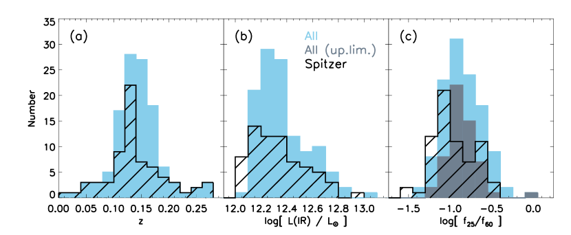
Figure 1.— Distributions of ($a$) redshifts, ($b$) infrared luminosities, and ($c$) 25-to-60µm flux ratios of the Spitzer 1 Jy ULIRGs (black hatched histogram) vs. entire 1 Jy sample (blue histogram). In panels ($b$) and ($c$), IRAS 12 and 25µm fluxes are used for the entire 1 Jy sample. Many of these fluxes are upper limits, which we label explicitly in panel ($c$). IRAS-type Spitzer 12 and 25µm fluxes are used for the Spitzer subsample. The new flux measurements account for the imperfect overlap in panels ($b$) and ($c$). The Spitzer ULIRGs are representative of the 1-Jy sample in both range and distribution of properties.

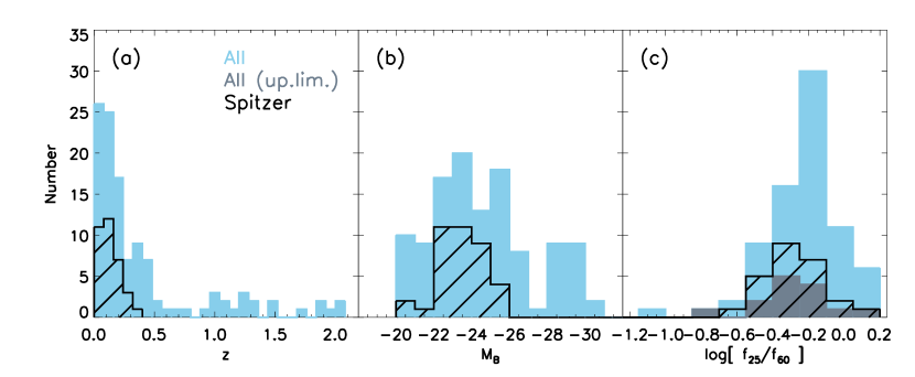
Figure 2.— Distributions of ($a$) redshifts, ($b$) B-band absolute magnitudes, and ($c$) 25-to-60 $\mu$m flux ratios of the Spitzer PG QSOs (black hatched histogram) vs. entire PG QSO sample (blue histogram). As in Figure 1, IRAS 25µm fluxes are used for the entire sample, and IRAS-type Spitzer fluxes for the current subsample. The Spitzer QSOs sample the low redshift and low luminosity ends of the PG QSO sample.

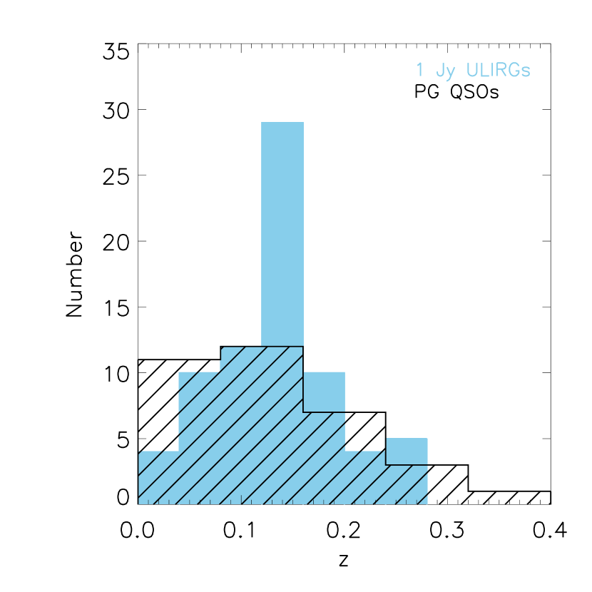
Figure 3.— Redshift distributions of the Spitzer ULIRGs (blue histogram) and PG QSOs (black hatched histogram). The two samples are well matched in redshift.

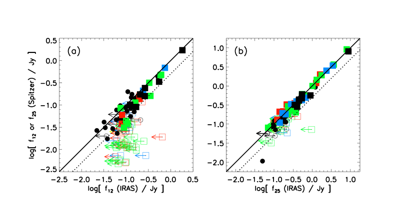
Figure 4.— Comparisons of IRAS ($a$) 12 and ($b$) 25 $\mu$m flux densities with Spitzer-derived quantities. Squares represent ULIRGs and circles are QSOs. Open symbols are upper limits. The colors of the symbols reflect the optical spectral types: red, green, blue, and black squares are HII-like, LINER, Seyfert 2, and Seyfert 1 ULIRGs, respectively. The solid line is perfect agreement, and the dotted line is for $f(IRAS)/f(Spitzer)=2$. Excellent agreement is seen at the 5% level at 25 $\mu$m and at the 25% level at 12 $\mu$m.

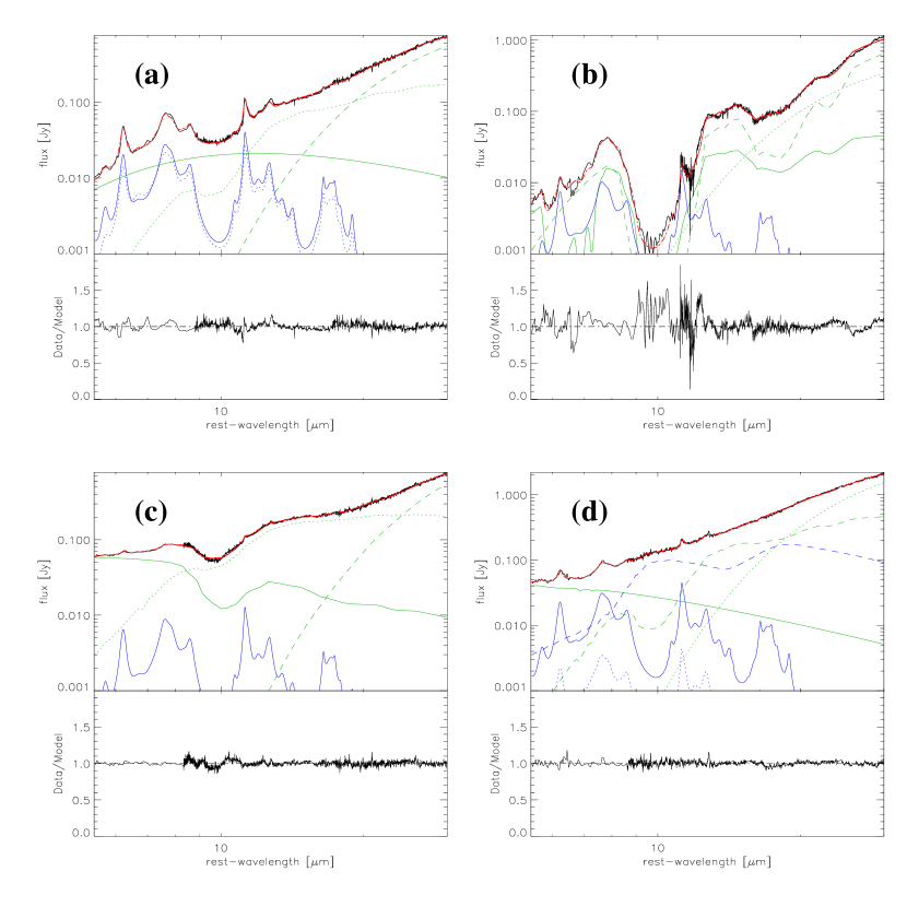
Figure 5.— Four examples of spectral decompositions: ($a$) PAH-dominated ULIRG, F15206+3342, ($b$) Highly obscured ULIRG, F00091$-$0738, ($c$) AGN-dominated ULIRG without silicate emission, F11119+3257, and ($d$) AGN-dominated ULIRG/PG QSO with silicate emission, Mrk 1014 = PG 0157+001. In each case, the top panel shows the fit to the IRS spectrum, while the bottom panel shows the data-to-model flux ratio. The data are in black, the overall fit is in red, the three blackbody components are in green, the two PAH templates are in blue, and the silicate emission component is the long-dash blue line. See Section 5.2 for more detail on the fits.

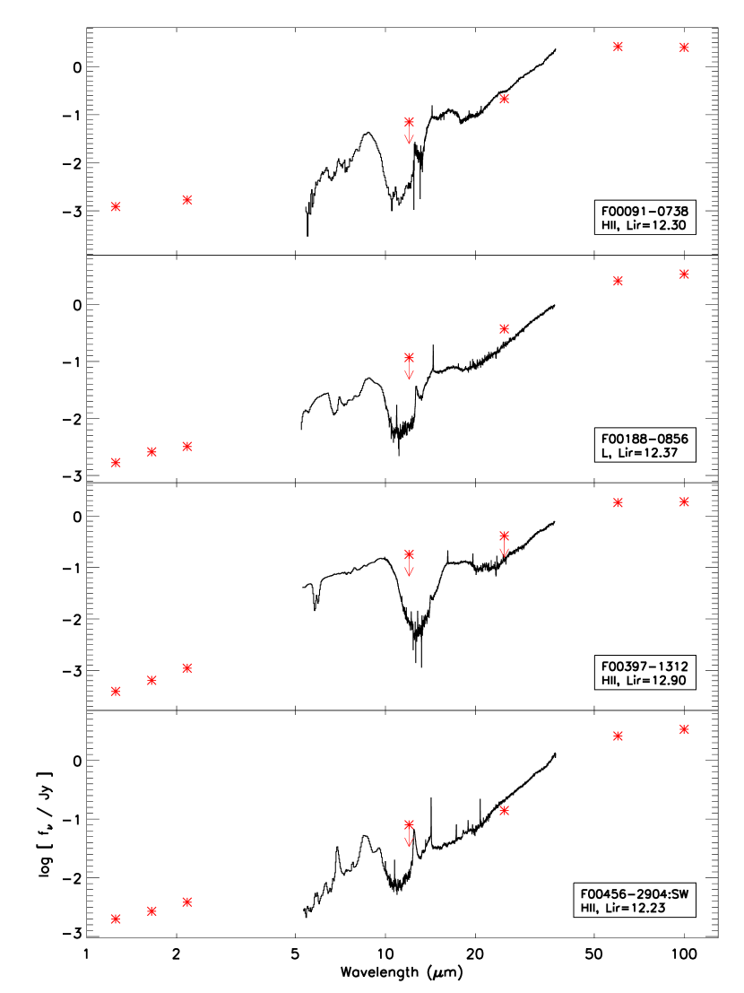
Figure 6.— IRS spectra of all ULIRGs considered in our study, in order of increasing right ascension. The sources of the overlaid photometry, shown as red stars, are discussed in Section 6. F11223$-$1244:W is shown in this figure but was mistakenly omitted from the analysis.

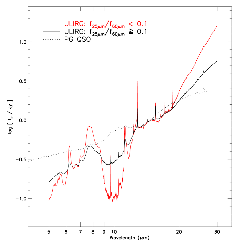
Figure 7.— Average IRS spectra for ULIRGs with 25-to-60 $\mu$m flux ratios, $f_{25}/f_{60}$, above and below 0.1, compared with the QSOs in our sample (Paper II). The individual spectra in each category were normalized to have the same rest-frame 15 $\mu$m flux density. Note the progression from cool ULIRGs to warm ULIRGs, and then to QSOs.

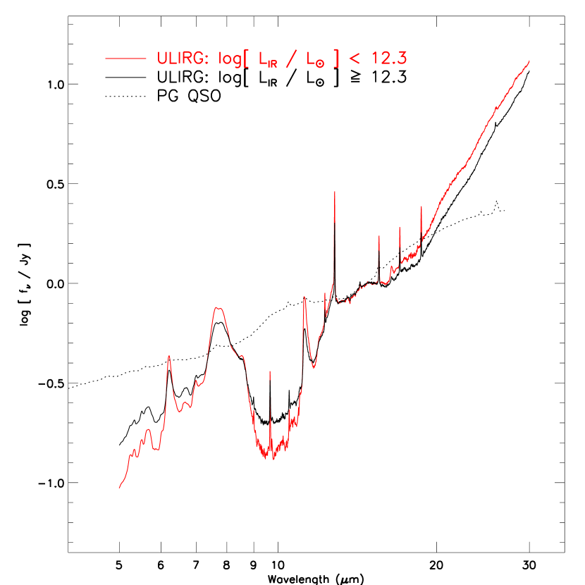
Figure 8.— Average IRS spectra for ULIRGs with infrared luminosities larger or smaller than 10^12.3 $L_{\odot}$, compared with the QSOs in our sample. The individual spectra in each category were normalized to have the same rest-frame 15 $\mu$m flux density.

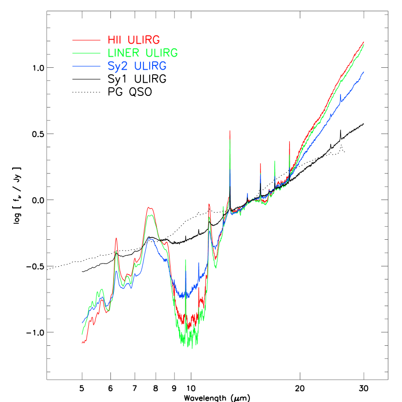
Figure 9.— Average IRS spectra for ULIRGs of various optical spectral types, compared with the QSOs in our sample. The individual spectra in each category were normalized to have the same rest-frame 15 $\mu$m flux density. Note the similarity between the average spectrum of Seyfert 1 ULIRGs and that of QSOs.

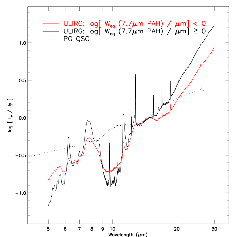
Figure 10.— Average IRS spectra for ULIRGs with PAH 7.7 $\mu$m equivalent widths larger or smaller than 1 µm, compared with the QSOs in our sample. The individual spectra in each category were normalized to have the same rest-frame 15 $\mu$m flux density.

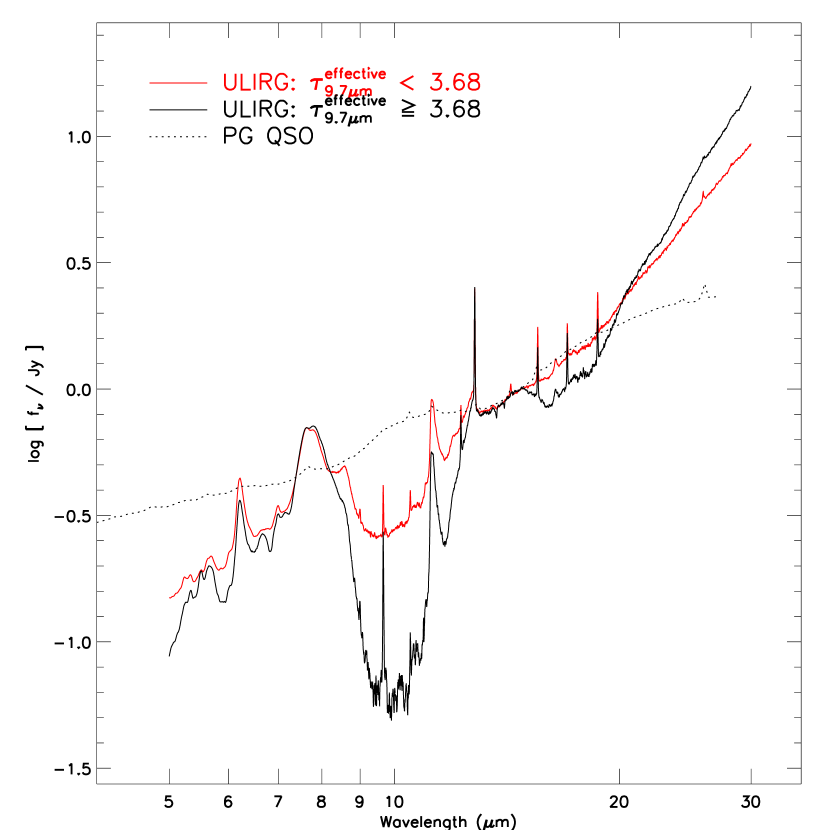
Figure 11.— Average IRS spectra for ULIRGs with effective optical depth of the 9.7 $\mu$m absorption feature larger or smaller than 3.68 (the sample median), compared with the QSOs in our sample. The individual spectra in each category were normalized to have the same rest-frame 15 $\mu$m flux density. Significant PAH emission is detected in both average ULIRG spectra.

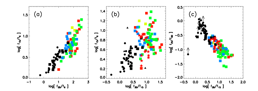
Figure 12.— MIR color-color diagrams: ($a$) 15-to-6 vs. 30-to-6 $\mu$m flux ratios, ($b$) 15-to-6 vs. 30-to-15 $\mu$m flux ratios, ($c$) 25-to-60 vs. 30-to-15 $\mu$m flux ratios. The meaning of the ULIRG and QSO symbols is the same as in Figure 4. In addition, the red stars and black triangles are starburst and Seyfert galaxies observed with $ISO$ (Verma et al. 2003; Sturm et al. 2002; Brandl et al. 2006). The tightest correlation is seen in ($c$).

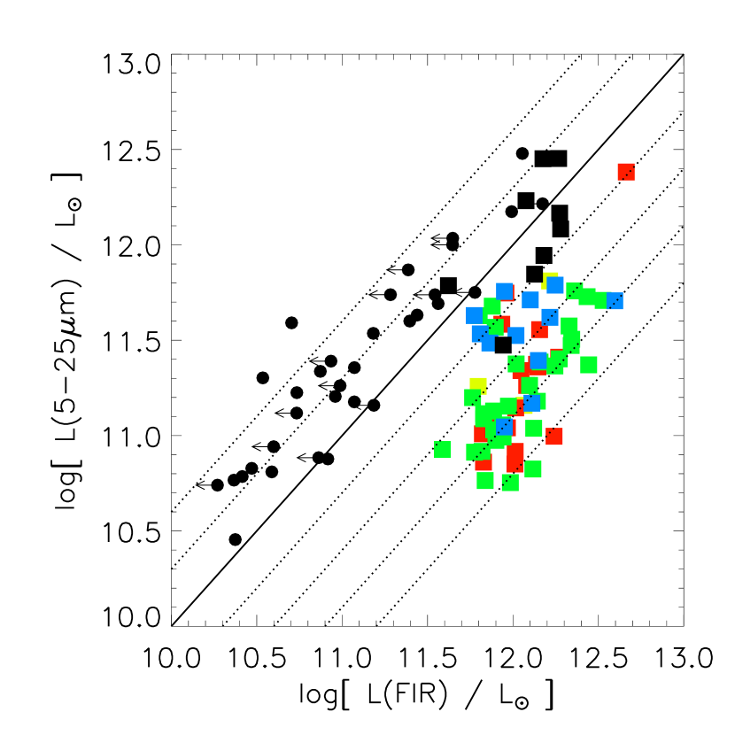
Figure 13.— Spitzer-derived MIR (5 – 25 $\mu$m) luminosities of 1-Jy ULIRGs and PG QSOs vs. FIR luminosities. The meaning of the symbols is the same as in Figure 4. The solid line is the line of equality, while the dashed lines show the locations of objects with FIR luminosities equal to (1/4, 1/2, 2, 4, 8, 16) $\times$ the MIR luminosities. All ULIRGs, except most of those that are optically classified as Seyfert 1s, are MIR underluminous relative to QSOs. Seyfert 2 ULIRGs are intermediate between QSOs/Seyfert 1 ULIRGs and HII-like/LINER ULIRGs. The HII-like ULIRG at very high infrared luminosity is F00397$-$1312, and has heavily extincted PAH emission.

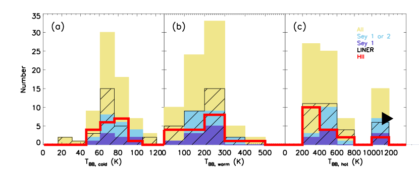
Figure 14.— Distributions of the blackbody temperatures for the ($a$) cold, ($b$) warm, and ($c$) hot components of the template fits to the IRS spectra of the 1-Jy ULIRGs. The arrowhead in panel ($c$) indicates that the somewhat uncertain $\sim$1000 K temperature are possibly lower limits (with an estimated range $\sim 700-2000$ K). The temperatures of the hot components in HII-like / LINER ULIRGs are distinctly lower than in Seyfert ULIRGs.

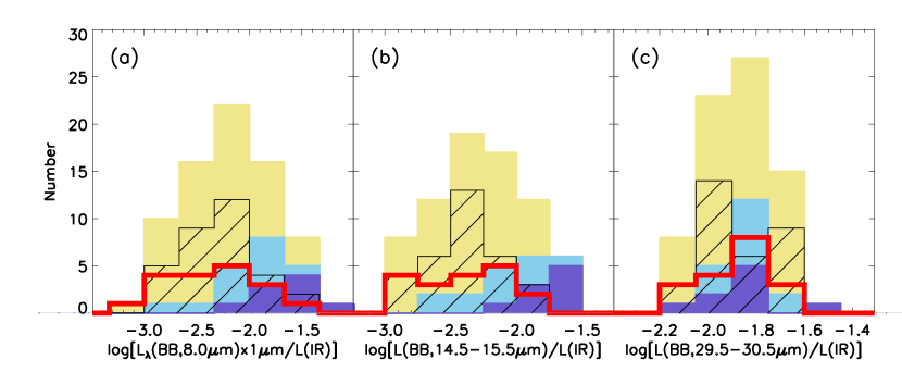
Figure 15.— Distributions of the ratios of the monochromatic blackbody (i.e., excluding PAH emission) ($a$) 8, ($b$) 15, and ($c$) 30 $\mu$m luminosities to the total infrared luminosities for 1-Jy ULIRGs of various optical spectral types (see the legend in Figure 14). The ratios involving the 8 and 15 $\mu$m luminosities are distinctly larger among Seyfert ULIRGs than among HII-like / LINER ULIRGs.

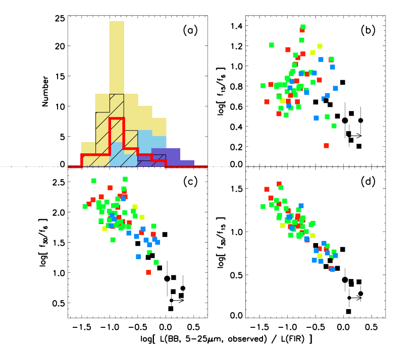
Figure 16.— ($a$) Distributions of the ratios of 5 – 25 $\mu$m blackbody (i.e., excluding PAH emission) luminosities to the FIR luminosities for 1-Jy ULIRGs of various optical spectral types (see the legend in Figure 14). This ratio is distinctly larger among Seyfert ULIRGs than among HII-like / LINER ULIRGs. ($b$, $c$, $d$) Ratios of 5 – 25 $\mu$m blackbody (i.e., excluding PAH emission) luminosities to the FIR luminosities for 1-Jy ULIRGs of various optical spectral types vs. 15-to-6 $\mu$m flux ratios ($b$), 30-to-6 $\mu$m flux ratios ($c$), and 30-to-15 $\mu$m flux ratios ($d$). The meaning of the symbols is the same as Figure 4. In addition, the small, medium-size, and large black circles correspond to the FIR-undetected, FIR-faint, and FIR-bright PG QSOs, respectively, as defined in Paper II. The strongest correlation is seen in ($d$).

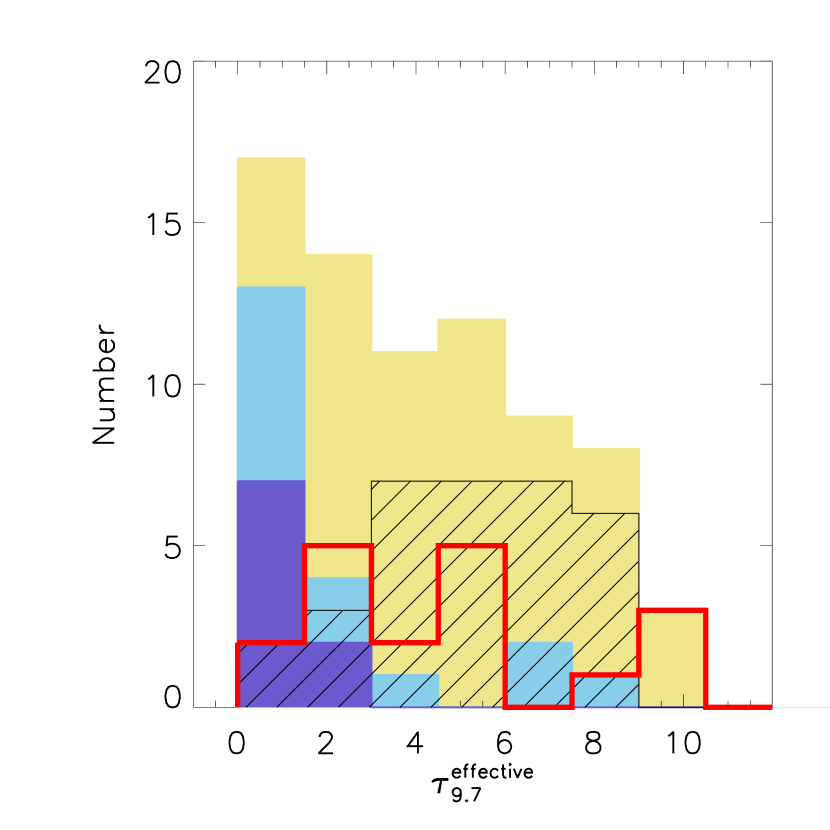
Figure 17.— Distributions of the effective 9.7 $\mu$m silicate optical depth for 1-Jy ULIRGs of various optical spectral types (see the legend in Figure 14). The four Seyfert 1 ULIRGs with silicate in emission are not shown in this figure. Optically classified Seyferts generally have smaller optical depths than HII-like/LINER ULIRGs.

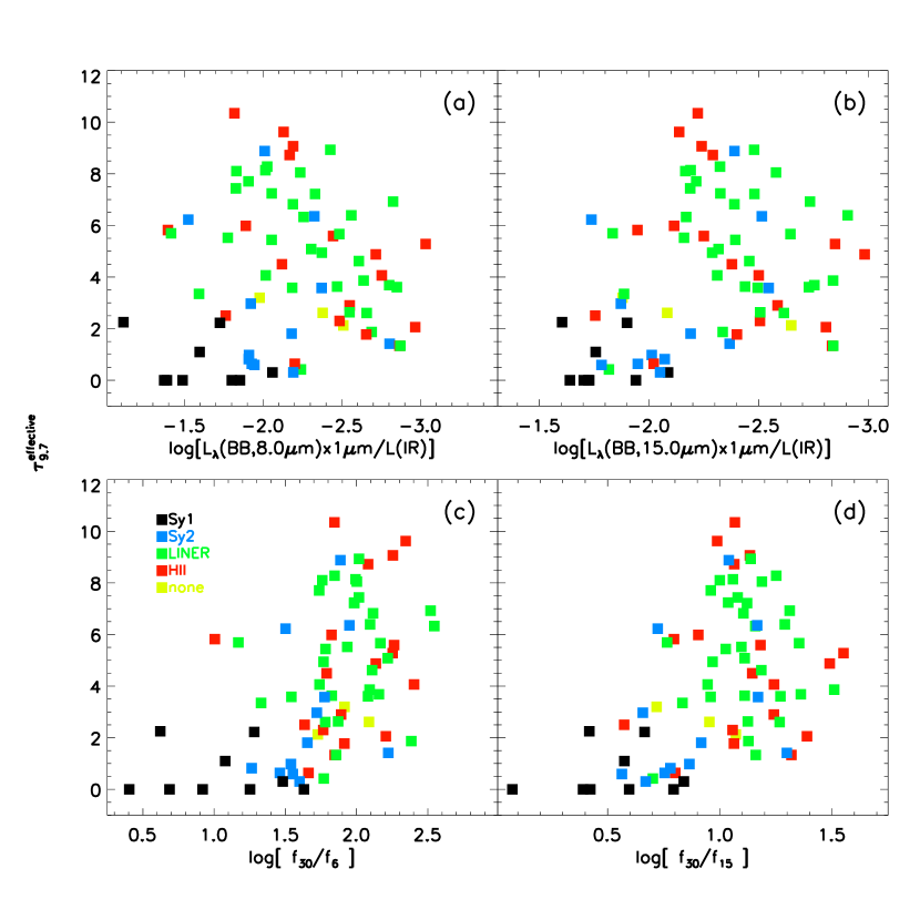
Figure 18.— Effective silicate optical depths vs. ($a$) ratios of monochromatic blackbody 8 $\mu$m luminosities to total infrared luminosities, ($b$) ratios of monochromatic blackbody 15 $\mu$m luminosities to total infrared luminosities, ($c$) 30-to-6 $\mu$m flux ratios, and ($d$) 30-to-15 $\mu$m flux ratios for the 1-Jy ULIRGs of various optical spectral types. The meaning of the symbols is the same as in Figure 4. Seyfert ULIRGs generally populate the lower left portion of these diagrams.

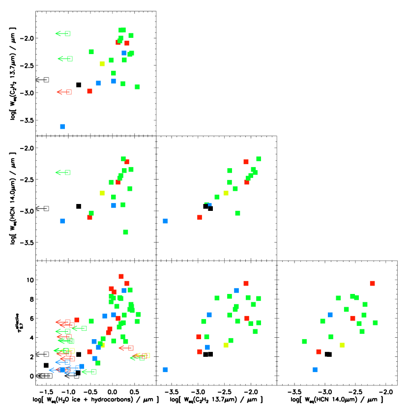
Figure 19.— Comparisons of absorption features: Effective optical depths of 9.7 $\mu$m silicate, equivalent widths of 14 $\mu$m HCN; equivalent widths of H₂O ice + hydrocarbons; equivalent widths of 13.7 $\mu$m C₂H₂, and equivalent widths of 14 $\mu$m HCN. The meaning of the symbols is the same as in Figure 4. The strengths of these features are only loosely correlated, implying significant variations in the composition of the dense absorbing material from one ULIRG to the next.

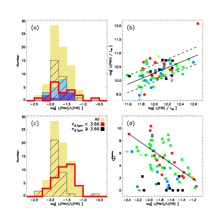
Figure 20.— ($a$),($c$) Distributions of the ratio of the total PAH luminosities to FIR luminosities of the 1-Jy ULIRGS according to optical spectral types (see the legend in Figure 14) and effective silicate optical depth (relative to the median value). There is a tight distribution (standard deviation 0.3 dex), as also illustrated in panel ($b$), where the PAH and FIR luminosities are plotted against each other. The meaning of the symbols is the same as in Figure 4, the solid line is the mean ratio assuming a slope of unity, and the dashed lines show the standard deviation from the mean. (The HII-like ULIRG that lies well above the best linear PAH-FIR fit is F00397$-$1312; the PAHs in this system are corrected for significant extinction.) This ratio is very similar to that of the PG QSOs (Paper I). ($d$) $L$(PAH)/$L$(FIR) vs. effective silicate optical depth. The line is a fit to HII/LINER ULIRGs. (F00397$-$1312, with the highest observed $L$(PAH)/$L$(FIR) value, is not visible in this plot). An anticorrelation exists between PAH/FIR ratio and silicate optical depth.

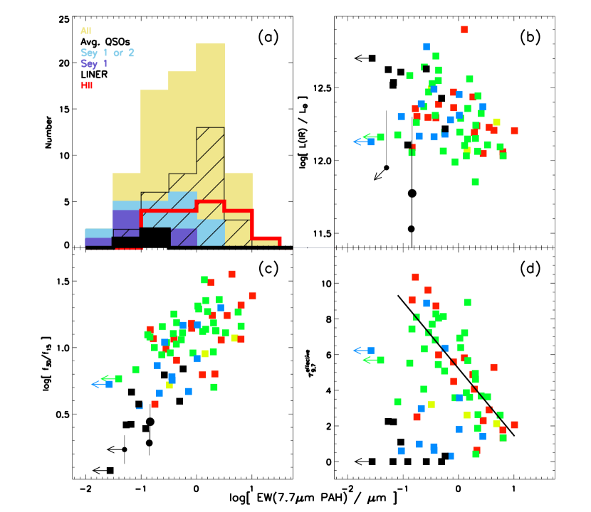
Figure 21.— ($a$) Distribution of equivalent widths of the 7.7 $\mu$m PAH feature for 1-Jy ULIRGs and average FIR-bright, FIR-faint, and FIR-undetected PG QSOs (see the legend in Figure 14). Note the similarity between Seyfert 1 ULIRGs and QSOs, and the higher EW(PAH) values in HII galaxies and LINERs than in Seyferts. In the other panels, the 7.7 $\mu$m PAH equivalent width is plotted as a function of ($b$) the infrared luminosity, ($c$) the 30-to-15 $\mu$m flux ratio, and ($d$) the silicate optical depth. The meaning of the square (circle) symbols is the same as in Figure 4 (16). These figures show that EW(PAH) is weakly correlated with infrared luminosity, strongly correlated with $f_{30}/f_{15}$ (more so than with optical spectral type), and strongly correlated with silicate optical depth for HII/LINER galaxies. The line in ($d$) is a fit to the HII/LINER detections. Seyferts deviate from the HII/LINER correlation and populate the lower left-hand corner of the plot.

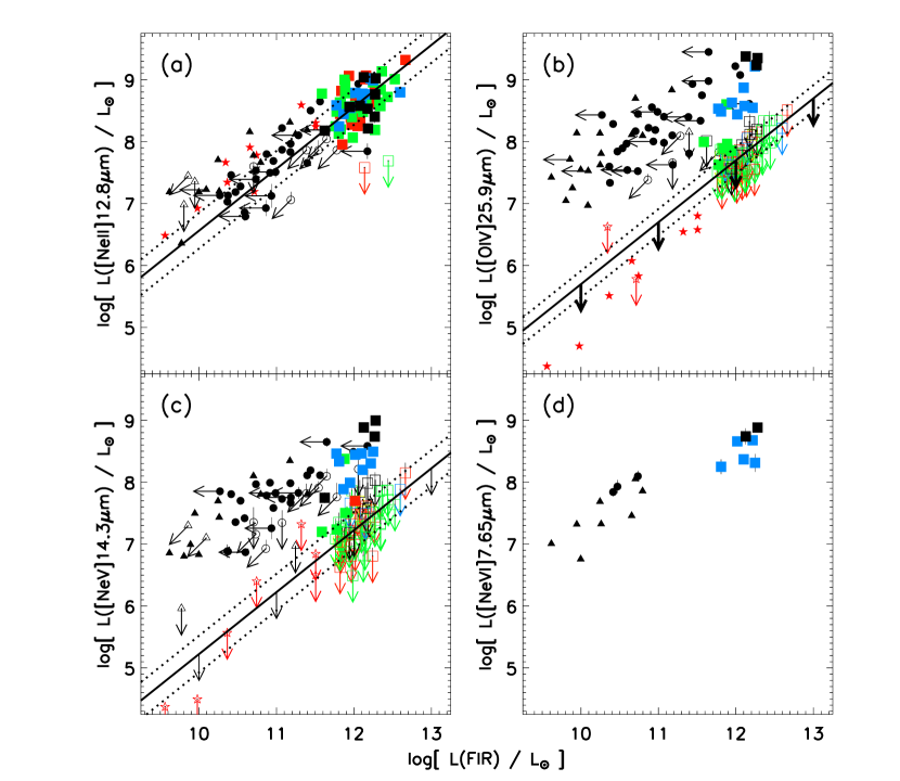
Figure 22.— ($a$) [Ne II] 12.8 $\mu$m luminosity, ($b$) [O IV] 25.9 $\mu$m luminosity, ($c$) [Ne V] 14.3 $\mu$m luminosity, and ($d$) [Ne VI] 7.65 $\mu$m luminosity vs. FIR luminosity of the 1-Jy ULIRGs and PG QSOs in the Spitzer sample as well as some optically-selected starbursts and Seyfert 2 galaxies observed with ISO. The meaning of the square and circle (other) symbols is the same as in Figure 4 (12). The solid (dotted) line represents the mean (standard deviation) of the ratio $L$(emission line)$/L$(FIR) for HII ULIRGs. All ULIRGs lie close to the fitted [Ne II]-to-FIR ratio of $10^{-3.4}$, but QSOs and Seyfert ULIRGs are increasingly above the values of the [O IV]- and [Ne V]-to-FIR luminosity ratios of HII ULIRGs. This result is readily explained if the AGN contributes increasingly to the fine-structure line emission at higher ionization levels.

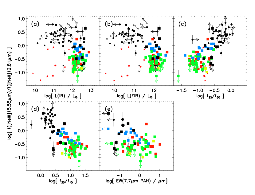
Figure 23.— [Ne III] 15.5 $\mu$m/[Ne II] 12.8 $\mu$m flux ratios vs. ($a$) total infrared luminosity, ($b$) FIR luminosity, ($c$) 25-to-60 $\mu$m flux ratio, ($d$) 30-to-15 $\mu$m flux ratio, and ($e$) 7.7 $\mu$m PAH equivalent width. The meaning of the small square and circle (other) symbols is the same as in Figure 4 (12 and 16). In addition, the small, medium-size, and large black circles in panel ($e$) correspond to the average FIR-undetected, FIR-faint, and FIR-bright PG QSOs from Paper II. No obvious trend is seen with FIR or total infrared luminosity among ULIRGs, but a clear dependence is seen on optical spectral type and IR continuum colors.

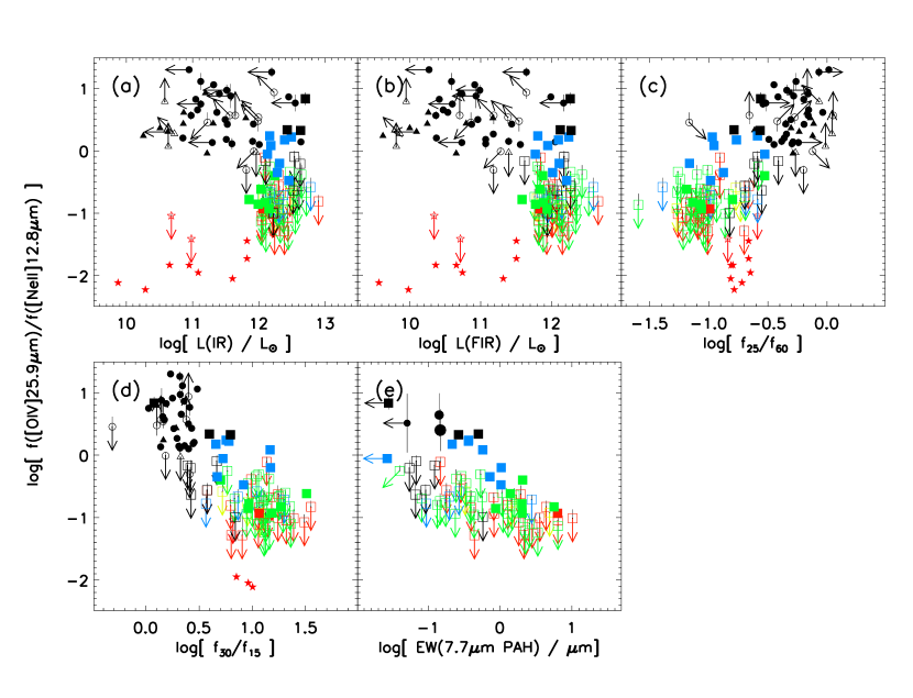
Figure 24.— [O IV] 25.9 $\mu$m/[Ne II] 12.8 $\mu$m flux ratios vs. ($a$) total infrared luminosity, ($b$) FIR luminosity, ($c$) 25-to-60 $\mu$m flux ratio, ($d$) 30-to-15 $\mu$m flux ratio, and ($e$) 7.7 $\mu$m PAH equivalent width. The meaning of the small square and circle (other) symbols is the same as in Figure 4 (12 and 16). This ratio among ULIRGs is slightly larger on average among ULIRGs with larger far- or total infrared luminosity. [O IV]/[Ne II] is more clearly larger among warmer, Seyfert ULIRGs. PG QSOs nicely fit along this excitation sequence.

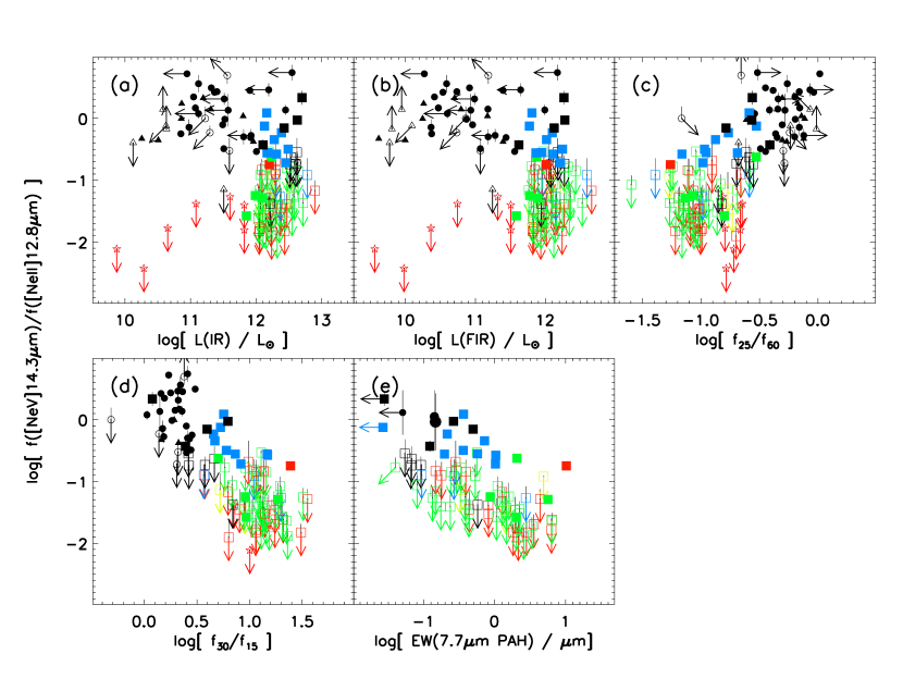
Figure 25.— [Ne V] 14.3 $\mu$m/[Ne II] 12.8 $\mu$m flux ratios vs. ($a$) total infrared luminosity, ($b$) FIR luminosity, ($c$) 25-to-60 $\mu$m flux ratio, ($d$) 30-to-15 $mu$m flux ratio, and ($e$) 7.7 $\mu$m PAH equivalent width. The meaning of the small square and circle (other) symbols is the same as in Figure 4 (12 and 16). This ratio among ULIRGs is slightly larger on average among ULIRGs with larger FIR or total infrared luminosity. [Ne V]/[Ne II] is more clearly larger among warmer, Seyfert ULIRGs. PG QSOs nicely fit along this excitation sequence.

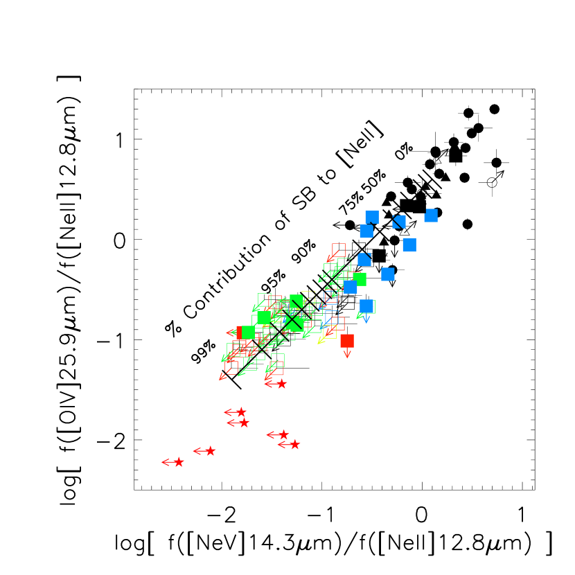
Figure 26.— [Ne V] 14.3 $\mu$m/[Ne II] 12.8 $\mu$m vs. [O IV] 25.9 $\mu$m/[Ne II] 12.8 $\mu$m for ULIRGs and PG QSOs in our sample. The meaning of the square and circle (other) symbols is the same as in Figure 4 (12). A clear positive correlation is observed, representing an excitation sequence anchored with the HII-like/LINER ULIRGs, moving up in excitation level to the Seyfert 2 and Seyfert 1 ULIRGs, and ending with the PG QSOs. The solid diagonal line in these diagrams indicates constant [Ne V]/[O IV] and changing [Ne II]. This line may be interpreted as a mixing line if [Ne V] and [O IV] are only produced by an AGN and [Ne II] by starburst activity. The tickmarks along the line indicate the percent contribution of the starburst to [Ne II]. The anchor point of this line has some systematic uncertainty due to variable AGN physical conditions.

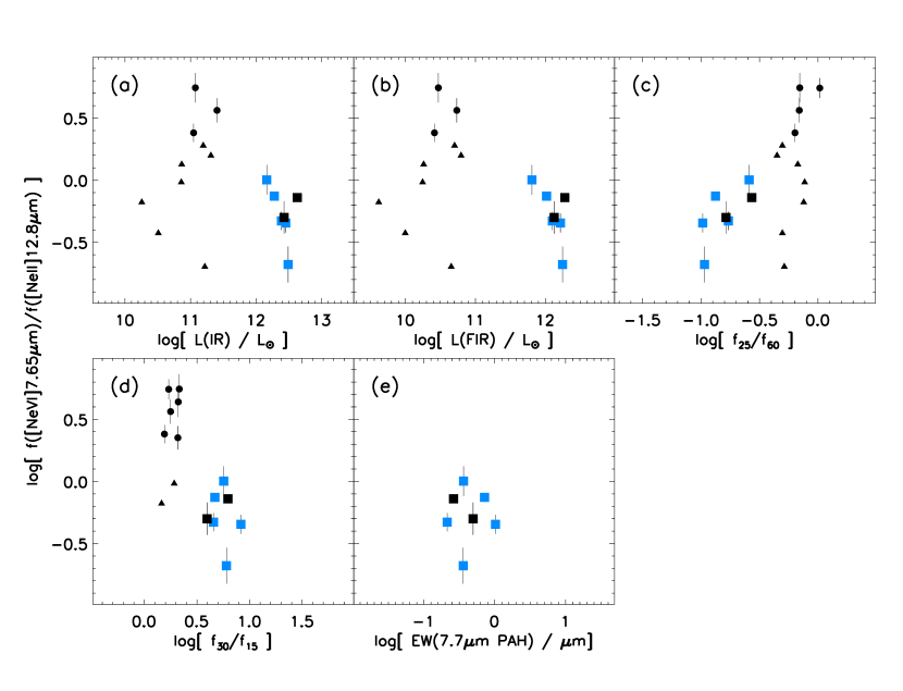
Figure 27.— [Ne VI] 7.65 $\mu$m/[Ne II] 12.8 $\mu$m flux ratios vs. ($a$) total infrared luminosity, ($b$) FIR luminosity, ($c$) 25-to-60 $\mu$m flux ratio, ($d$) 30-to-15 $\mu$m flux ratio, and ($e$) 7.7 $\mu$m PAH equivalent width. The meaning of the square and circle (triangle) symbols is the same as in Figure 4 (12). [Ne VI] is detected only in Seyfert ULIRGs and QSOs. The small number of detections prevent us from looking for statistically significant correlations with infrared or FIR luminosity, optical spectral type, or continuum colors.

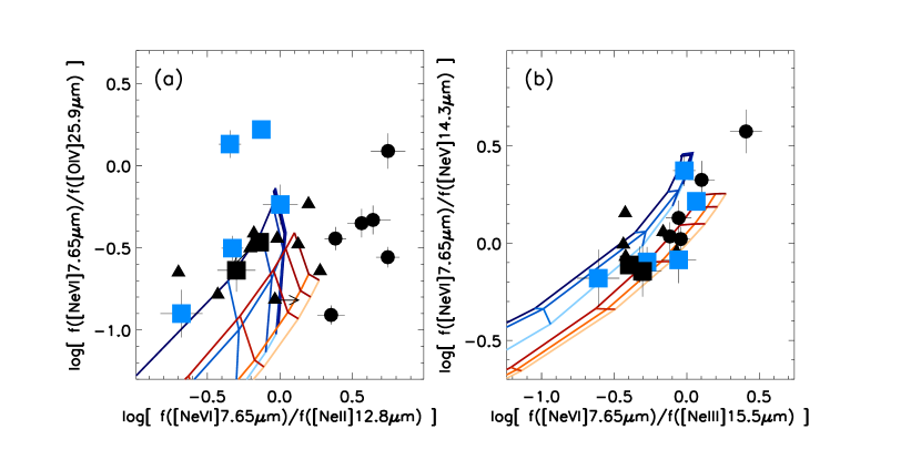
Figure 28.— ($a$) [Ne VI] 7.65 $\mu$m/[Ne II] 12.8 $\mu$m vs. [Ne VI] 7.65 $\mu$m/[O IV] 25.9 $\mu$m and ($b$) [Ne VI] 7.65 $\mu$m/[Ne III] 15.5 $\mu$m vs. [Ne VI] 7.65 $\mu$m/[Ne V] 14.3 $\mu$m for ULIRGs and PG QSOs in our sample. The meaning of the square and circle (triangle) symbols is the same as in Figure 4 (12). The grids show the predictions from the dusty, solar-metallicty, radiation pressure-dominated photoionization models of Groves et al. (2004) for two different power-law slopes [$f_{\nu}\propto\nu^{\alpha}$, $\alpha=-1.2$ (blue) and $\alpha=-2.0$ (red)]. The two parameters that vary across the grids are the ionization parameter (log $U$ = $-$4 – 0) and the hydrogen density (log $n_{H}$ = 2 – 4). The color hues correspond to low values (light color) and high values (dark color); e.g., dark blue means high density or high ionization parameter. Poor agreement is seen in ($a$) due to starburst contamination of [Ne II] or problems with the model (highlighted by disagreements in both axes). Panel ($b$) is more useful, since it uses only high ionization lines of a single element (Ne). The good agreement means that AGN may power not only [Ne VI] and [Ne V], but also [Ne III], in these systems.

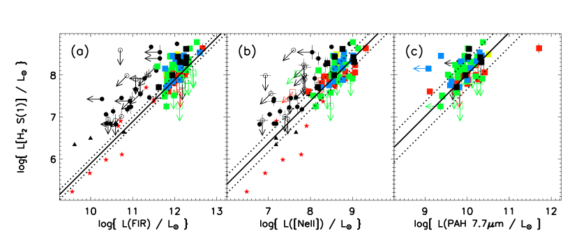
Figure 29.— Luminosity of H₂ S(1) 17.04 $\mu$m vs. various star formation indicators: ($a$) FIR luminosity, ($b$) luminosity of [Ne II] 12.8 $\mu$m, and ($c$) luminosity of PAH 7.7 $\mu$m. The meaning of the square and circle (other) symbols is the same as in Figure 4 (12). The solid and dotted lines show the mean and standard deviation of $L$[H₂ S(1)]/$L$(X) (where X $=$ FIR, etc.) for HII ULIRGs. A positive correlation is seen between these quantities for both ULIRGs and PG QSOs. However, Seyfert ULIRGs and especially PG QSOs have larger H₂-to-FIR, H₂-to-[Ne II], and H₂-to-PAH ratios than HII ULIRGs, suggesting that H₂ emission is influenced by the presence of the AGN in these objects. The LINERs also have significantly larger ratios and dispersions in panels ($b$) and ($c$).

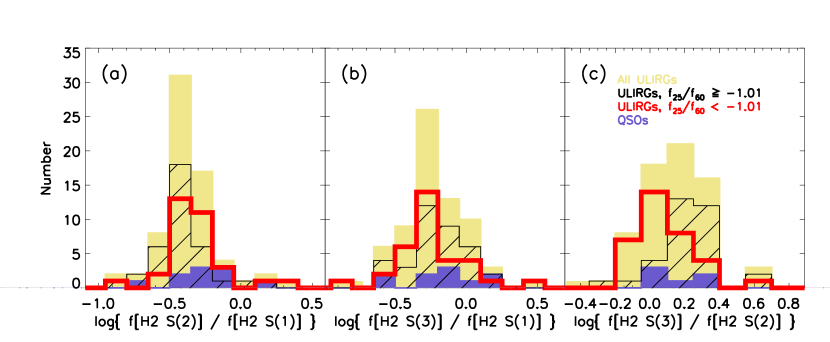
Figure 30.— Histograms of H₂ ($a$) S(2)/S(1), ($b$) S(3)/S(1), and ($c$) S(3)/S(2) flux ratios (uncorrected for extinction) as a function of $f_{25}/f_{60}$ in ULIRGs and QSOs. The ULIRG distributions are divided at the median value of $f_{25}/f_{60}$. These ratios are indicative of the excitation temperature of H₂ gas, but can also be affected by extinction and variable ortho-to-para ratios. Warm ULIRGs have smaller S(2)/S(1) ratios on average than cool ULIRGs by 0.1 dex, with a K-S (Kuiper) probability of arising from the same distribution of $<$0.1% (1%). Warm ULIRGs have larger S(3)/S(2) ratios on average than cool ULIRGs by 0.15 dex, with a K-S (Kuiper) probability of arising from the same distribution of $<$0.1% (2%). Warm and cool ULIRGs are statistically indistinguishable in S(3)/S(1).

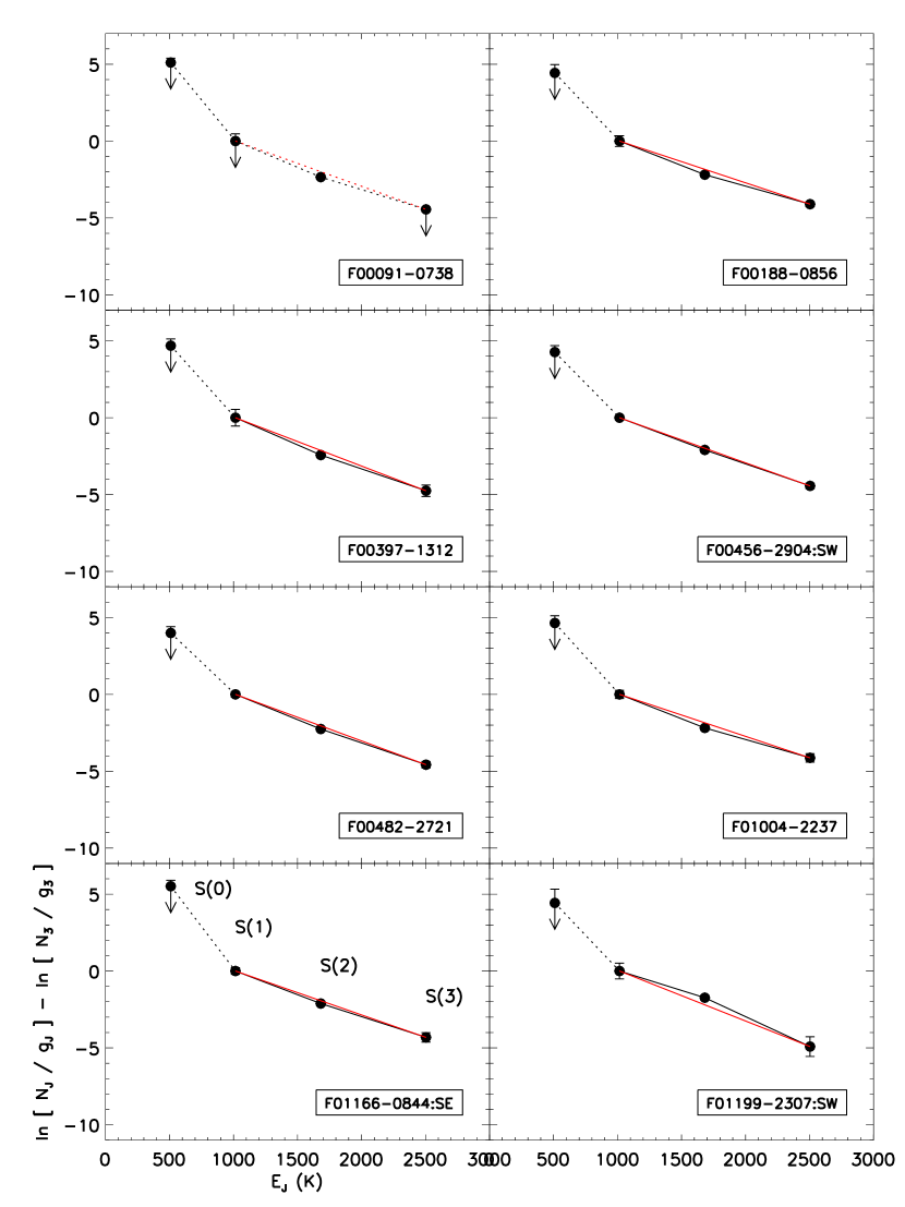
Figure 31.— H₂ excitation diagram for a few ULIRGs in our sample. The excitation temperature ($T_{ex}$) is the reciprocal of the slope between any two data points. Solid lines join points where both lines are detected, and dashed lines join points where at least one line is an upper limit. Black lines join immediately adjacent lines, and red lines join the the S(1) and S(3) transitions. Error bars are 2$\sigma$.

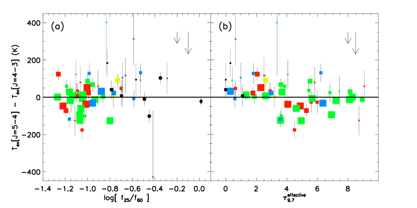
Figure 32.— Difference between the excitation temperatures derived from the H₂ S(3)/S(2) and S(2)/S(1) flux ratios vs. ($a$) $f_{25}/f_{60}$ and ($b$) the 9.7 $\mu$m silicate effective optical depth. The meaning of the symbols is the same as in Figure 4. The size of the symbol reflects the relative uncertainties on each data point, where the quartile of most certain points are the largest and the quartile of least certain points are the smallest. All objects should be above the solid line, unless extinction and/or ortho-para effects are at play. The small downward arrow on the right in each diagram reflects the effect of changing the ortho-to-para ratio from 3 to 2, while the long arrow reflects the effect of an extinction $A_{V}=10$. Significant trends among ULIRGs are seen, with decreasing temperature difference with increasing silicate optical depth and decreasing $f_{25}/f_{60}$. ULIRGs with extinction greater than the median (and $f_{25}/f_{60}$ lower than the median) have a lower temperature difference by $60-70$ K, with a K-S (Kuiper) significance of $<$0.1% (6$-$7%). The trend with extinction implies extinction of the molecular lines. When corrected for this extinction, the trend with $f_{25}/f_{60}$ will lessen or disappear.

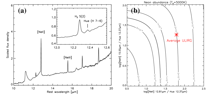
Figure 33.— ($a$) Average IRS spectrum of PAH-dominated ULIRGs from Figure 10, minus one object with high obscuration (F00397$-$1312). The average spectrum is from individual spectra normalized at 15 µm. The zoomed-in insert shows the detection of Hu$\alpha$ 12.4 $\mu$m. ($b$) [Ne III] 15.5 $\mu$m/Hu$\alpha$ and [Ne II] 12.8 $\mu$m/Hu$\alpha$ ratios derived from this average spectrum. The neon abundance relative to hydrogen increases from the lower-left portion of this diagram to the upper-right, as indicated by the solid iso-metallicity curves. The line ratios of the average spectrum suggest a neon abundance $\sim$2.9 $\times$ solar, based on the Asplund et al. (2004) normalization (see text for a discussion of the uncertainties on this value).

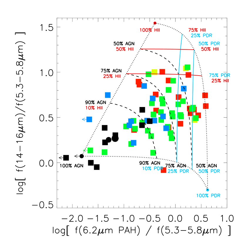
Figure 34.— AGN/HII/PDR mixing diagram based on the Laurent et al. (2000) method, as modified by Armus et al. (2007): PAH (6.2 $\mu$m) to continuum (5.3 – 5.8 $\mu$m) flux ratios vs. the continuum (14 – 16 $\mu$m) / (5.3 – 5.8 $\mu$m) flux ratios. The meaning of the symbols is the same as in Figure 4. The zero points for the pure HII region (upper-right) and PDR (lower-right) are from Armus et al. (2007) and the zero point for the pure AGN (lower-left) corresponds to the average value for the FIR-undetected PG QSOs to reduce possible starburst contributions to the continuum emission (Paper II). Note that the percentages included here are percentages of the $5.3-5.8$ µm continuum; actual AGN fractional contributions to the bolometric luminosities will be lower.

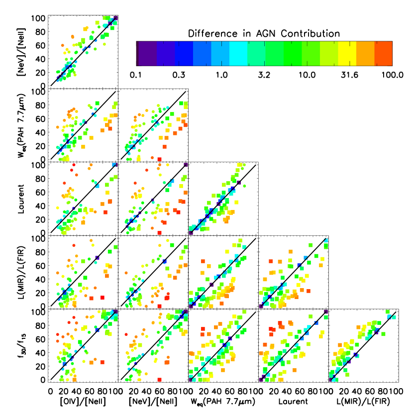
Figure 35.— Comparison of AGN fractional contributions to the bolometric luminosities of ULIRGs and PG QSOs derived from 6 different methods: the ([O IV] 25.9 $\mu$m/[Ne II] 12.8 $\mu$m) ratio, the ([Ne V] 14.3 $\mu$m/[Ne II] 12.8 $\mu$m) ratio, the equivalent width of PAH 7.7 $\mu$m, the PAH (5.9 - 6.8 $\mu$m) to continuum (5.1 – 6.8 $\mu$m) flux ratio combined with the continuum (14 – 15 $\mu$m) / (5.1 – 5.8 $\mu$m) flux ratio, the MIR blackbody to FIR flux ratio, and the $f_{30}/f_{15}$ continuum flux ratio. Squares are actual AGN fractional contributions, while small circles are upper limits on the AGN fractional contributions derived from the fine structure line ratios. The colors represent deviations ($x-y$) from the line of equality, on a logarithmic scale. Good agreement is seen on average between the various methods. See Appendix A, Section 7.1.1, and Tables $\ref{tab:agnfrac_zp}-\ref{tab:agnfrac_indiv}$ for a description of each method and the results of these comparisons.

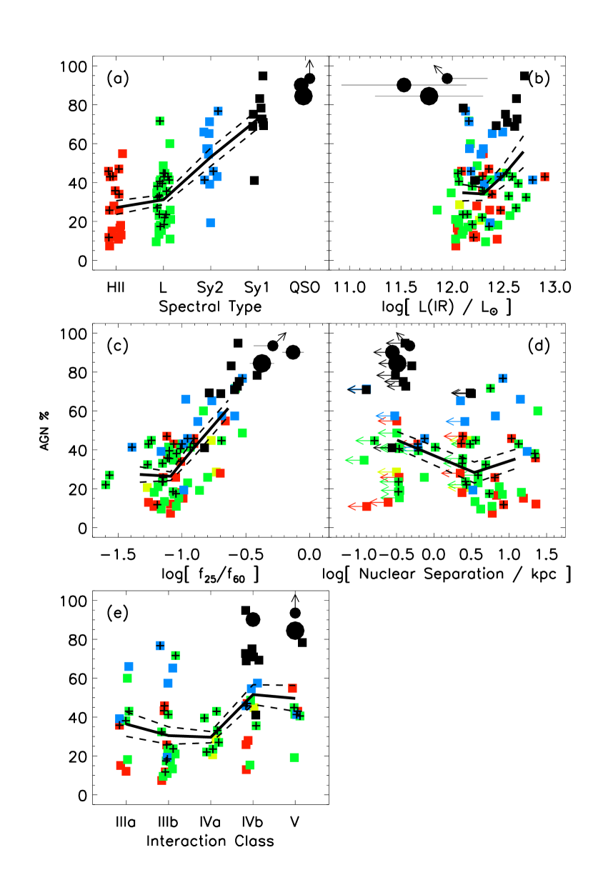
Figure 36.— AGN fractional contributions to the bolometric luminosities of ULIRGs and PG QSOs, averaged over all 6 methods, vs. (a) optical spectral type; (b) infrared luminosity; (c) $f_{25}/f_{60}$; (d) nuclear separation; and (e) interaction class. The meaning of the small square (large circle) symbols is the same as in Figure 4 (16). Overlaid crosses indicate ULIRGs with higher than average MIR extinction. The average ($\pm$1 standard error) AGN contributions in each horizontal bin are connected by the solid (dashed) lines. These binned points include ULIRGs only. The scatter in spectral type and interaction class [panels ($a$) and ($e$)] is added artificially for clarity. Strong positive correlations are detected between AGN contribution and optical spectral type / continuum slope: more Seyfert-like and warmer galaxies are increasingly AGN-dominated. Weaker, though significant, trends are seen for the other 3 independent variables: AGN contribution is highest at the highest infrared luminosities, smallest nuclear separations, and latest interaction classes. In all cases but infrared luminosity, the addition of PG QSOs either extends or enhances these trends.

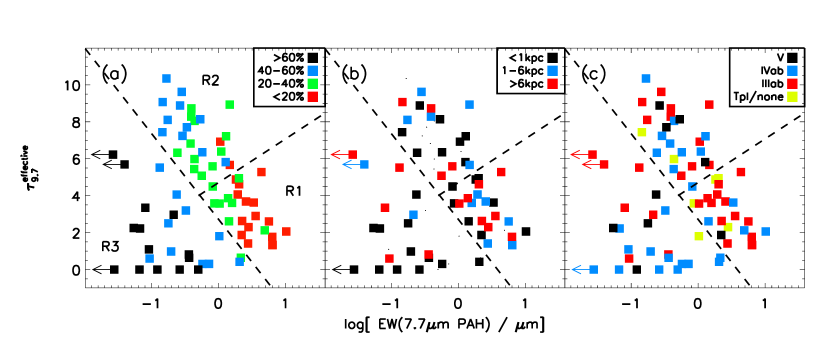
Figure 37.— Effective optical depth of the 9.7 $\mu$m silicate feature vs. equivalent width of the 7.7 $\mu$m PAH feature as a function of (a) AGN fractional contribution to bolometric luminosity, (b) nuclear separation, and (c) interaction class. The meaning of the symbols is the same as in Figure 4. For clarity, we divide this diagram into three regions of roughly equal numbers. AGN contribution increases as one moves from Region 1 through Region 2 and into Region 3. There is also a trend toward smaller nuclear separations and later merger stage along the sequence R1 $-$ R2 $-$ R3, but it is a weak trend with significant scatter (see Table 13).

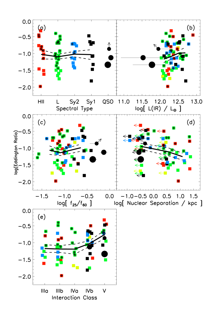
Figure 38.— Eddington ratio from photometry vs. (a) optical spectral type; (b) infrared luminosity; (c) $f_{25}/f_{60}$; (d) nuclear separation; and (e) interaction class. The meaning of the small square (large circle) symbols is the same as in Figure 4 (16). Overlaid crosses indicate ULIRGs with higher than average MIR extinction. The average ($\pm$1 standard error) Eddington ratios in each horizontal bin are connected by the solid (dashed) lines. These binned points include ULIRGs only. The scatter in spectral type and interaction class [panels ($a$) and ($e$)] is added artificially for clarity. There are no obvious correlations between Eddington ratios and any of these paramters. The Eddington ratios appear to be highest at the smallest nuclear separations and latest interaction classes, and the addition of PG QSOs seems to either extend or enhance these trends, but these results cannot be confirmed in a more rigorous statistical analysis.

Figure 39.— Eddington ratio from photometry vs. (a) optical spectral type; (b) infrared luminosity; (c) $f_{25}/f_{60}$; (d) nuclear separation; and (e) interaction class. The meaning of the small square (large circle) symbols is the same as in Figure 4 (16). Overlaid crosses indicate ULIRGs with higher than average MIR extinction. The average ($\pm$1 standard error) Eddington ratios in each horizontal bin are connected by the solid (dashed) lines. These binned points include ULIRGs only. The scatter in spectral type and interaction class [panels ($a$) and ($e$)] is added artificially for clarity. There are no obvious correlations between Eddington ratios and any of these paramters. The Eddington ratios appear to be highest at the smallest nuclear separations and latest interaction classes, and the addition of PG QSOs seems to either extend or enhance these trends, but these results cannot be confirmed in a more rigorous statistical analysis.

References

- (1) Abel, N. P., & Satyapal, S. 2008, ApJ, 678, 686 Armus, L., et al. 2004, ApJS, 154, 178 Armus, L., et al. 2007, ApJ, 656, 148 Asplund, M., Grevesse, N., Sauval, A. J., Allende Prieto, C., & Kiselman, D. 2004, A&A, 417, 751 Barnes, J. E. 1989, Nature, 338, 123 Barnes, J. E. 2004, MNRAS, 350, 798 Barnes, J. E., & Hernquist, L. 1996, ApJ, 471, 115 Beswick, R. J., Pedlar, A., Mundell, C. G., Gallimore, J. F. 2001, MNRAS, 325, 151 Blain, A. W., Smail, I., Ivison, R. J., Kneib, J.-P., & Frayer, D. T. 2002, Phys. Rep., 369, 111 Boroson, T., & Green, R. 1992, ApJS, 80, 109 Bournaud, F., Jog, C. J., & Combes, F. 2005, A&A, 437, 69 Brandl, B. R., et al. 2006, ApJ, 653, 1129 Butler, K., & Zeippen, C. J. 1994, A&AS, 108, 1 Calzetti, D., et al. 2007, ApJ, 666, 870 Cao, C., et al. 2008, MNRAS, 390, 336 Chiar, J. E., & Tielens, A. G. G. M. 2006, ApJ, 637, 774 Cox, T. J., Jonsson, P., Primack, J. R., & Somerville, R. S. 2006, MNRAS, 373, 1013 Daddi, E., et al. 2007, ApJ, 670, 156 Dale, D. A., et al. 2006, ApJ, 646, 161 Dasyra, K. M., et al. 2006a, ApJ, 638, 745 Dasyra, K. M., et al. 2006b, ApJ, 651, 835 Dasyra, K. M., et al. 2007, ApJ, 657, 102 Davies, R. I., et al. 2007, ApJ, 671, 1388 de Grijp, M. H. K., Miley, G. K., Lub, J., & de Jong, T. 1985, Nature, 314, 240 Dekel, A., & Birnboim, Y. 2008, MNRAS, 383, 119 Dekel, A., et al. 2009, Nature, 457, 451 Desai, V., et al. 2007, ApJ, 669, 810 Di Matteo, T., Springel, V., & Hernquist, L. 2005, Nature, 433, 604 Dopita, M. A., et al. 2006, ApJ, 639, 788 Downes, D. & Solomon, P. M. 1998, ApJ, 507, 615 Drake, J. J., & Testa, P. 2005, Nature, 436, 525 Engelbracht, C. W., et al. 2005, ApJ, 628, L29 Evans, A. S., Frayer, D. T., Surace, J. A., & Sanders, D. B. 2001, AJ, 121, 1893 Evans, A. S., Mazzarella, J. M., Surace, J. A., & Sanders, D. B. 2002, ApJ, 580, 749 Evans, A. S., Solomon, P. M., Tacconi, L. J., Vavilkin, T., & Downes, D. 2006, AJ, 132, 2398 Farrah, D., Surace, J. A., Veilleux, S., Sanders, D. B., & Vacca, W. D. 2005, ApJ, 626, 70 Farrah, D., et al. 2007, ApJ, 667, 149 Ferrarese, L., & Merritt, D. 2000, ApJ, 539, L9 Förster Schreiber, N. M., Roussel, H., Sauvage, M., & Charmandaris, V. 2004, A&A, 419, 501 Förster Schreiber et al. 2006, ApJ, 645, 1062 Förster Schreiber et al. 2009, preprint (astro-ph/0903.1872) Gebhardt, K., et al. 2000, ApJ, 539, L13 Genel, S., et al. 2008, ApJ, 688, 789 Genzel, R., et al. 1998, ApJ, 498, 579 Genzel, R., et al. 2001, ApJ, 563, 527 Genzel, R., et al. 2006, Nature, 442, 786 Genzel, R., et al. 2008, ApJ, 687, 59 Groves, B., Dopita, M., & Sutherland, R. 2004, A&A, 458, 405 Guélin, M., et al. 2007, A&A, 462, L45 Guyon, O., Sanders, D. B., & Stockton, A. 2006, ApJS, 166, 89 Hao, L., et al. 2007, ApJ, 655, L77 Helou, G., et al. 2001, ApJ, 548, L73 Herbst, T. M., Beckwith, S. V. W., Glindemann, A., Tacconi-Garman, L. E., Kroker, H., & Krabbe, A. 1996, AJ, 111, 2403 Higdon, S. J. U., Armus, L., Higdon, J. L., Soifer, B. T., & Spoon, H. W. W. 2006, ApJ, 648, 323 Higdon, S. J. U., et al. 2004, PASP, 116, 975 Hony, S., Van Kerckhoven, C., Peeters, E., Tielens, A. G. G. M., Hudgins, D. M., & Allamandola, L. J. 2001, A&A, 370, 1030 Houck, J. R., et al. 2004, ApJS, 154, 19 Imanishi, M., Dudley, C. C., Maloney, P. R. 2006a, ApJ, 637, 114 Imanishi, M., Nakanishi, K., & Kohno, K. 2006b, AJ, 131, 2888 Imanishi, M., et al. 2007, ApJS, 171, 72 Imanishi, ., et al. 2008, PASJ, 60, 489 Iono, D., Yun, M. S., & Mihos, J. C. 2004, ApJ, 616, 199 Kennicutt, R. C. 1998, ARA&A, 36, 189 Kim, D.-C., & Sanders, D. B. 1998, ApJS, 119, 41 Kim, D.-C., Veilleux, S., & Sanders, D. B. 1998, ApJ, 508, 627 Kim, D.-C., Veilleux, S., & Sanders, D. B. 2002, ApJS, 143, 277 Klaas, U., et al. 2001, A&A, 379, 823 Kormendy, J., & Sanders, D. B. 1992, ApJ, 388, L9 Lahuis, F., & van Dishoeck, E. F. 2000, A&A, 355, 699 Lahuis, F., et al. 2006, ApJ, 636, L145 Lahuis, F., et al. 2007, ApJ, 659, 296 Laurent, O., et al. 2000, A&A, 359, 887 Levenson, N. A., et al. 2007, ApJ, 654, L45 Li, M. P., Shi, Q. J., & Li, A. 2008, MNRAS, 391, L49 Lonsdale, C. J., Farrah, D., & Smith, H. E. 2006, Astrophysics Update 2, ed. J. W. Mason, Springer Verlag, Heidelberg, Germany, p. 285 Lu, N., et al. 2003, ApJ, 588, 199 Lutz, D., Kunze, D., Spoon, H. W. W., & Thornley, M. D. 1998a, 333, 75 Lutz, D., Spoon, H. W. W., Rigopoulou, D., Moorwood, A. F. M., & Genzel, R. 1998b, ApJ, 505, L103 Lutz, D., Veilleux, S., & Genzel, R. 1999, ApJ, 517, L13 Lutz, D., et al. 2003, A&A, 409, 867 Marconi, A., & Hunt, L. K. 2003, ApJ, 589, L21 Martin, C. L. 2005, ApJ, 621, 227 Mihos, J. C., & Hernquist, L. 1996, ApJ, 464, 641 Mihos, J. C., McGaugh, S. S., & de Blok, W. J. G. 1997, ApJ, 477, L79 Naab, T., Jesseit, R., & Burkert, A. 2006, MNRAS, 372, 839 Netzer, H., et al. 2007, ApJ, 666, 806 (Paper II) O’Halloran, B., Satyapal, S., & Dudik, R. P. 2006, ApJ, 641, 795 Peeters, E., Spoon, H. W. W., & Tielens, A. G. G. M. 2004, ApJ, 613, 986 Puxley, P. J., Brand, P. W. J. L., Moore, T. J. T., et al. 1989, ApJ, 345, 163 Rigby, J. R., & Rieke, G. H. 2004, ApJ, 606, 237 Rigopoulou, D., et al. 1999, AJ, 118, 2625 Rigopoulou, D., et al. 2002, A&A, 389, 374 Risaliti, G., et al. 2006, MNRAS, 365, 303 Rossa, J., et al. 2007, AJ, 134, 2124 Roussel, H., et al. 2007, ApJ, 669, 959 Rupke, D. S. N., Veilleux, S., & Sanders, D. B. 2002, ApJ, 570, 588 Rupke, D. S. N., Veilleux, S., & Sanders, D. B. 2005a, ApJS, 160, 87 Rupke, D. S. N., Veilleux, S., & Sanders, D. B. 2005b, ApJS, 160, 115 Rupke, D. S. N., Veilleux, S., & Sanders, D. B. 2005c, ApJ, 632, 751 Rupke, D. S. N., Veilleux, S., & Baker, A. J. 2008, ApJ, 674, 172 Sajina, A., et al. 2007, ApJ, 664, 713 Sakamoto, K., Scoville, N. Z., Yun, M. S., Crosas, M., Genzel, R., & Tacconi, L. J. 1999, ApJ, 514, 68 Sanders, D. B., Mazzarella, J. M., Kim, D.-C., Surace, J. A., & Soifer, B. T. 2003, AJ, 126, 1607 Sanders, D. B., & Mirabel, L. F. 1996, ARA&A, 34, 749 Sanders, D. B., Soifer, B. T., Elias, J. H., Neugebauer, G., & Matthews, K. 1988b, ApJ, 328, L35 Sanders, D. B., et al. 1988a, ApJ, 325, 74 Sani, E., et al. 2008, ApJ, 675, 96 Saraph, H. E., & Tully, J. A. 1994, A&AS, 107, 29 Schmelz, J. T., et al. 2005, ApJ, 634, L197 Schmidt, M., & Green, R. F. 1983, ApJ, 269, 352 Schweitzer, M., et al. 2006, ApJ, 649, 79 (Paper I) Schweitzer, M., et al. 2008, ApJ, 679, 101 (Paper III) Scoville, N. Z., et al. 2000, AJ, 119, 991 Scoville, N. Z., Frayer, D. T., Schinnerer, E., & Christopher, M. 2003, ApJ, 585, l105 Shapiro, K., et al. 2008, ApJ, 682, 231 Sirocky, M. M., et al. 2008, ApJ, 678, 729 Smith, J. D. T., et al. 2007, ApJ, 656, 770 Soifer, B. T., et al. 2000, AJ, 119, 509 Soifer, B. T., et al. 2002, AJ, 124, 2980 Solomon, P. M., Downes, D., Radford, S. J. E., & Barrett, J. W. 1997, ApJ, 478, 144 Spoon, H. W. W., et al. 2001, A&A, 365, L353 Spoon, H. W. W., et al. 2002, A&A, 385, 102 Spoon, H. W. W., et al. 2004, ApJS, 154, 184 Spoon, H. W. W., et al. 2006, ApJ, 638, 759 Spoon, H. W. W., et al. 2007, ApJ, 654, L49 Springel, V., Di Matteo, T., & Hernquist L. 2005, ApJ, 620, L79 Storey, P. J., & Hummer, D. G. 1995, MNRAS, 272, 41 Sturm, E., et al. 2002, A&A, 393, 821 Sturm, E., et al. 2005, ApJ, 629, L21 Sturm, E., et al. 2006, ApJ, 653, L13 Surace, J. A. 1998, Ph. D. thesis, University of Hawaii Surace, J. A., & Sanders, D. B. 1999, AJ, 512, 162 Surace, J. A., Sanders, D. B., & Evans, A. S. 2001, AJ, 122, 2791 Surace, J. A., Sanders, D. B., Vacca, W. D., Veilleux, S., & Mazzarella, J. M. 1998, ApJ, 492, 116 Surace, J. A., et al. 2006, Proceedings of the 2005 Lijiang Conference, “The Spitzer Space Telescope”: New Views of the Cosmos”, eds. L. Armus and W. T. Reach, Pub. A. S. P., 357, 223 Tacconi, L. J., et al. 2002, ApJ, 580, 73 Tacconi, L. J., et al. 2006, ApJ, 640, 228 Tacconi, L. J., et al. 2008, ApJ, 680, 246 Taniguchi, Y., Yoshino, A., Ohyama, Y., & Nishiura, S. 1999, ApJ, 514, 660 Thornley, M. D., et al. 2000, ApJ, 539, 641 Tielens, A. G. G. M., Hony, S., van Kerckhoven, C., & Peeters, E. 1999, in The Universe as Seen by ISO, ed. P. Cox & M. F. Kessler (ESA SP-427; Noordwijk: ESA), 579 Toomre, A., & Toomre, J. 1972, ApJ, 178, 623 Tran, Q. D., et al. 2001, ApJ, 552, 527 Tremaine, S., et al. 2002, ApJ, 574, 740 van Kerckhoven, C., et al. 2000, A&A, 357, 1013 Veilleux, S., Cecil, G., & Bland-Hawthorn, J. 2005, ARA&A, 43, 769 Veilleux, S., Kim, D.-C., & Sanders, D. B. 2002, ApJS, 143, 315 Veilleux, S., Kim, D.-C., & Sanders, D. B. 1999a, ApJ, 522, 113 Veilleux, S., Kim, D.-C., Sanders, D. B., Mazzarella, J. M., Soifer, B. T. 1995, ApJS, 98, 171 Veilleux, S., Sanders, D. B., & Kim, D.-C. 1997, ApJ, 477, 631 Veilleux, S., Sanders, D. B., & Kim, D.-C. 1999b, ApJ, 522, 139 Veilleux, S., et al. 2006, ApJ, 643, 707 Veilleux, S., et al. 2009, ApJ, submitted Verma, A., et al. 2003, A&A, 403, 829 Voit, G. M. 1992, MNRAS, 258, 841 Wang, W., & Liu, X.-W. 2008, MNRAS, 389, L33 Wright, G. S., James, P. A., Joseph, R. D., & McLean, I. 1990, Nature, 344, 417 Younger, J. D., Hopkins, P. F., Cox, T. J., & Hernquist, L. 2008, ApJ, 686, 815