Beyond standard Poisson-Boltzmann theory: ion-specific interactions in aqueous solutions

Abstract

The Poisson-Boltzmann mean-field description of ionic solutions has been successfully used in predicting charge distributions and interactions between charged macromolecules. While the electrostatic model of charged fluids, on which the Poisson-Boltzmann description rests, and its statistical mechanical consequences have been scrutinized in great detail, much less is understood about its probable shortcomings when dealing with various aspects of real physical, chemical and biological systems. These shortcomings are not only a consequence of the limitations of the mean-field approximation per se, but perhaps are primarily due to the fact that the purely Coulombic model Hamiltonian does not take into account various additional interactions that are not electrostatic in their origin. We explore several possible non-electrostatic contributions to the free energy of ions in confined aqueous solutions and investigate their ramifications and consequences on ionic profiles and interactions between charged surfaces and macromolecules.

1 Introduction

The traditional approach to ions in solution has been the mean-field Poisson-Boltzmann (PB) formalism. This approach adequately captures the main features of electrostatic interactions at weak surface charges, low ion valency, and high temperature [1, 2]. It stems from a Coulombic model Hamiltonian that includes only purely electrostatic interactions between different charged species. The limitations of the PB approach, which rests on a collective and continuous description of statistical charge distributions become particularly important in highly-charged systems, where counterion-mediated interactions between charged bodies cannot be described by the mean-field approach that completely neglects ion correlations and charge fluctuations [3]. These mean-field limitations have been successfully bypassed and have led to more refined descriptions that capture some of the important non-mean-field aspects of Coulomb fluids [4].

Beside electrostatic interactions that are universal, omnipresent non-electrostatic interactions are specific and dependent on the nature of the ionic species, solvent and confining interfaces. Because it is difficult, perhaps impossible, to devise a universal theory accounting for all non-electrostatic effects, such additional interactions need to be treated separately, describing specific electrolyte features that go beyond regular PB theory. These effects depend on ionic chemical nature, size, charge, polarizability and solvation (preferential ion-solvent interaction [7]).

In this review we describe how adding non-electrostatic terms in the system free energy yields modified PB equations and ionic density profiles and differentiate between the way different ionic species interact with macromolecules. While it has long been recognized that ions can have such different effects on macromolecular interactions [8], only recently have such ionic features been accounted for within electrostatic mean-field theory. Examples include ion effects on surface tension [9] and precipitation of proteins from solutions [10]. The latter led to the so-called Hofmeister ranking of different ions according to their surface activity. Adsorption of ions and/or surfactants to charged interfaces also contains substantial contributions from non-electrostatic degrees of freedom, as was shown within the Ninham-Parsegian theory of charge regulation at surfaces [11].

The outline of this paper is as follow. After reviewing the standard PB theory in section 2, we present in section 3 how addition of steric effects result in saturation of ionic profiles close to charged interfaces. In section 4 we show how non-electrostatic interactions between ions and charged membranes can cause a phase transition between two lamellar systems of different periodicity. Solvation effects are the topic discussed in section 5, where local variation of the dielectric function in solvent mixtures and ion-solvent interactions lead to changes in ionic and solvent profiles close to charged interfaces. Finally, in section 6 possible polarization effects of ions in solution is added to their ionic character, again resulting in different behavior close to charge interfaces.

2 The Poisson-Boltzmann model: summary and main results

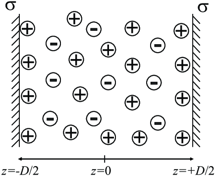
Figure 1: Schematic illustration of the model system. The two plates residing at $z=\pm D/2$ are charged with surface charge density $\sigma$. The electrolyte ions are denoted by $\oplus$ and $\ominus$. Their densities are $n_{+}(z)$ and $n_{-}(z)$.

The PB theory is a useful starting point for many theoretical ramifications because it relies on a simple and analytically tractable model that can be easily extended and amended. Although the theory has its own well-understood limitations, it yields meaningful results in good agreement with many experiments [1].

The model can be cast in many geometries but we shall focus on the simplest planar system, as depicted in figure 1. Two charged planar plates (of infinite extent), located at $z=\pm D/2$, are immersed in an electrolyte bath. Each plate carries a charge density of $\sigma$ (per unit area) and their inter-surface separation $D$ is a tunable system parameter. The ionic solution is denoted as $z_{+}{:}z_{-}$ and is composed of a solvent of dielectric constant $\varepsilon$ and two types of ions: cations of valency $z_{+}$ and local density (number per unit volume) $n_{+}(z)$, and anions of valency $z_{-}$ with local density $n_{-}(z)$. The finite system of thickness $D$ is in contact with an electrolyte bath of bulk densities $n_{\pm}^{b}$ obeying the electroneutrality condition: $z_{+}n^{b}_{+}=z_{-}n^{b}_{-}$. Throughout the paper, we will use the convention that $z_{-}$ (denotes the valency of the anions) is taken as a positive number, hence, their respective charge is written as ${-}ez_{-}$.

The free energy within the PB model $F_{\rm PB}$ can be derived in numerous ways as can be found in the literature [1]. With our notation $F_{\rm PB}$ is a function of the densities $n_{\pm}$ and the local electrostatic potential $\psi$:

$$F_{\rm PB} = \int\mathrm{d}^{3}r\left[-\frac{\varepsilon}{8\pi}(\nabla\psi)^{2}+(z_{+}n_{+}-z_{-}n_{-})e\psi\right]$$ (1)

$$+ k_{\mathrm{B}}T\int\mathrm{d}^{3}r\left[n_{+}\ln(a^{3}n_{+})+n_{-}\ln(a^{3}n_{-})-n_{+}-n_{-}\right]$$

$$- \int\mathrm{d}^{3}r\left[\mu_{+}n_{+}+\mu_{-}n_{-}\right]$$

The above free energy is a functional of three independent fields: $n_{\pm}$ and $\psi$. The first integral in (1) is the electrostatic energy, while the second represents the ideal mixing entropy of a dilute solution of the $\pm$ ions. Note that a microscopic length scale $a$ was introduced in the entropy terms above. Only one such microscopic length scale will be used throughout this paper, defining a reference density associated with close-packing ${n_{0}}=1/a^{3}$.

The last integral in (1) is written in terms of the chemical potentials $\mu_{\pm}$ of the $\pm$ ions. Alternatively, the chemical potential can be regarded as a Lagrange multiplier, setting the bulk densities to be $n_{\pm}^{b}=\exp(\mu_{\pm}/k_{\mathrm{B}}T)/a^{3}$.

The thermodynamic equilibrium state is given by minimizing the above free energy functional. Taking the variation of the free energy (1) with respect to $n_{\pm}$ yields the Boltzmann distribution of the ions in the presence of the local potential $\psi$:

$$\frac{\delta F_{\rm PB}}{\delta n_{\pm}} = \pm ez_{\pm}\psi+k_{\mathrm{B}}T\ln(n_{\pm}a^{3})-\mu_{\pm}=0$$ (2)

wherefrom

$$n_{\pm}=n_{\pm}^{b}\exp\left(\mp ez_{\pm}\psi/k_{\mathrm{B}}T\right)$$ (3)

Similarly, taking the variation with respect to the potential $\psi$ yields the Poisson equation connecting $\psi$ with the $\pm$ densities:

$$\frac{\delta F_{\rm PB}}{\delta\psi} = \frac{\varepsilon}{4\pi}\nabla^{2}\psi+ez_{+}n_{+}-ez_{-}n_{-}=0$$ (4)

Combining the Boltzmann distribution with the Poisson equation yields the familiar Poisson-Boltzmann equation:

$$\nabla^{2}\psi=-\frac{4\pi e}{\varepsilon}\left[z_{+}n_{+}^{b}\rme^{-ez_{+}\psi/k_{\mathrm{B}}T}\,-\,z_{-}n_{-}^{b}\rme^{ez_{-}\psi/k_{\mathrm{B}}T}\,\right]$$ (5)

that serves as a starting point for various extensions presented in the sections to follow.

In addition to the volume contribution (1) of the free energy, we need to include a surface electrostatic energy term $F_{s}$, which couples the surface charge density $\sigma$ with the surface value of the potential $\psi(z{=}\pm D/2)=\psi_{s}$. This surface term has the form

$$F_{s}=\int_{\rm A}\mathrm{d}^{2}r\,\sigma\psi_{s}$$ (6)

and takes into account the fact that we work in an ensemble where the surface charge density is fixed. Variation of $F_{\rm PB}+F_{s}$ with respect to $\psi_{s}$ yields the well-known electrostatic boundary condition

$$\frac{\delta}{\delta\psi_{s}}(F_{\rm PB}+F_{s})=\frac{\varepsilon}{4\pi}\mathbf{\hat{n}}\cdot{\nabla}\psi\,+\,\sigma=0$$ (7)

wherefrom

$$\mathbf{\hat{n}}\cdot{\nabla}\psi=-\frac{4\pi}{\varepsilon}\sigma$$ (8)

where $\mathbf{\hat{n}}$ is a unit vector normal to the surface. This boundary condition can also be interpreted as the electroneutrality condition since the amount of mobile charge should exactly compensate the surface charge.

The above PB equation is valid in any geometry. But if we go back to the planar case with two parallel plates, it is straightforward to calculate the local pressure $P_{\rm PB}$ at any point $z$ between the plates. In chemical equilibrium $P_{\rm PB}$ should be a constant throughout the system. Namely, $P_{\rm PB}$ is independent of the position $z$ and can be calculated by taking the proper variation of the free energy with respect to the inter-plate spacing $D$:

$$P_{\rm PB}=-\frac{\varepsilon}{8\pi}(\psi^{\prime})^{2}+k_{\mathrm{B}}T\left(n_{+}+n_{-}\right)$$ (9)

The pressure is composed of two terms. The first is the electrostatic pressure stemming from the Maxwell stress tensor. This term is negative, meaning an attractive force contribution acting between the plates. The second term originates from the ideal entropy of mixing of the ions and is positive. This term is similar to an “ideal gas” van ’t Hoff osmotic pressure of the $\pm$ species.

A related relation can be obtained from (9) for one charged surface. Comparing the pressure $P_{\rm PB}$ calculated at contact with the charge surface, with the distal pressure ($z\to\infty$) results in the so-called Graham equation used in colloid and interfacial science [12]

$$\sigma^{2}=\frac{\varepsilon k_{\mathrm{B}}T}{2\pi}(n_{+}^{s}+n_{-}^{s}-n_{+}^{b}-n_{-}^{b})$$ (10)

where $n_{\pm}^{s}$ are the values of the counterion and co-ion densities calculated at the surface.

Note that the osmotic pressure as measured in experiments can be written as the difference between the local pressure and the electrolyte bath pressure:

$$\Pi=P_{\rm PB}-k_{\mathrm{B}}T\left(n_{+}^{b}+n_{-}^{b}\right)$$ (11)

We now mention two special cases separately: the counterion only case and the linearized Debye-Hückel theory.

2.1 The counterion only case

In the counterion only case no salt is added to the solution and there are just enough counterions to balance the surface charge. For this case we have chosen arbitrarily the sign of the surface charge to be negative, $\sigma<0$. By setting $n_{+}\equiv 0$, the free energy is written only in terms of the anion density in solution, $n\equiv n_{-}$ and $z_{-}=z$

$$F_{\rm PB}=\int\mathrm{d}^{3}r\left[-\frac{\varepsilon}{8\pi}(\nabla\psi)^{2}-ezn\psi+k_{\mathrm{B}}T(n\ln\frac{n}{n_{0}}-n)\right]$$ (12)

The local pressure $P_{\rm PB}$ also contains only osmotic pressure of one type of ions ($n_{-}$), apart from the Maxwell stress term.

2.2 The linearized Debye-Hückel theory

When the surface charges and potentials are small, $e\psi_{s}\ll k_{\mathrm{B}}T$ ($\psi_{s}\ll 25$ mV at room temperature), the PB equation can be linearized and matches the Debye-Hückel theory. For the simple and symmetric $1{:}1$ monovalent electrolytes the PB equation reduces to:

$$\nabla^{2}\Psi=\lambda_{\mathrm{D}}^{-2}\Psi$$ (13)

where the dimensionless potential is defined as $\Psi=e\psi/k_{\mathrm{B}}T$ and the Debye screening length is $\lambda_{\mathrm{D}}=\sqrt{\varepsilon k_{\mathrm{B}}T/8\pi e^{2}n_{b}}$. The main importance of the Debye length $\lambda_{\mathrm{D}}$ is to indicate a typical length for the exponential decay of the potential around charged objects and boundaries: $\Psi(z)\sim\exp(-z/\lambda_{\mathrm{D}})$. The $\lambda_{\mathrm{D}}$ length is about 3Å for $n_{b}=1$ M of NaCl and about 1$\mu$m for pure water. It is convenient to express the Debye length in term of the Bjerrum length $l_{\mathrm{B}}=e^{2}/\varepsilon k_{\mathrm{B}}T$ as $\lambda_{\mathrm{D}}=\sqrt{1/8\pi l_{\mathrm{B}}n_{b}}$. For water at room temperature $l_{\mathrm{B}}\simeq 7$Å.

Returning now to the general non-linear PB model, its free energy (1) can also be expressed in terms of the dimensionless potential $\Psi$. For a 1:1 symmetric electrolyte we write it as:

$$F_{\rm PB}/k_{\mathrm{B}}T = \int\mathrm{d}^{3}r\left[-\frac{1}{8\pi l_{\mathrm{B}}}(\nabla\Psi)^{2}+(n_{+}-n_{-})\Psi\right]$$ (14)

$$+ \int\mathrm{d}^{3}r\left[n_{+}\ln(n_{+}/n_{b})+n_{-}\ln(n_{-}/n_{b})\right.$$

$$- \left.n_{+}-n_{-}+2n_{b}\right]$$

where the bulk contribution to the free energy is subtracted in the above expression.

In the next sections we will elaborate on several extensions and modifications of the PB treatment. Results in terms of ion profiles and inter-surface pressure will be presented and compared to the bare PB results.

3 Steric effects: finite ion size

At sufficiently high ionic densities steric effects prevent ions from accumulating at charged interfaces to the extent predicted by the standard PB theory. This effect has been noted already in the work of Eigen [13], elaborated later in [14] and developed into a final form by Borukhov et al. [15] and more recently in [16]. Steric constraints lead to saturation of ion density near the interface and, thus, increase their concentration in the rest of the interfacial region. This follows quite generally from the energy-entropy competition: the gain from the electrostatic energy is counteracted by the entropic penalty associated with ion packing. Beyond the mean-field (e.g., integral equation closure approximations), the correlations in local molecular packing clearly lead to ion layering and non-monotonic interactions between interfaces [17, 18].

Steric effects lead to a modified ionic entropy that in turn gives rise to a modified Poisson–Boltzmann (MPB) equation, governing the distribution of ions in the vicinity of charged interfaces. The main features of the steric effect can be derived from a lattice-gas model introduced next [19]. Other possible approaches that were considered include the Stern layer modification of the PB approach, extensive MC simulations or numeric solutions of the integral closures relations [20].

We start with a free energy where the entropy of mixing is taken in its exact lattice-gas form, without taking the dilute solution limit. Instead of point-like particles, the co-ions and counter-ions are now modeled as finite-size particles having the same radius $a$. The free energy for a $z_{+}{:}z_{-}$ electrolyte is now a modification of $F_{\rm PB}$ (1):

$$F_{\rm MPB} = \int\mathrm{d}^{3}r\left[-\frac{\varepsilon}{8\pi}(\nabla\psi)^{2}+(z_{+}n_{+}-z_{-}n_{-})e\psi\right]$$ (15)

$$+k_{\mathrm{B}}T\int\mathrm{d}^{3}r\left[n_{+}\ln(a^{3}n_{+})+n_{-}\ln(a^{3}n_{-})\right]$$

$$+\frac{k_{\mathrm{B}}T}{a^{3}}\int\mathrm{d}^{3}r\,(1-a^{3}n_{+}-a^{3}n_{-})\ln(1-a^{3}n_{+}-a^{3}n_{-})$$

$$-\int\mathrm{d}^{3}r\left[\mu_{+}n_{+}+\mu_{-}n_{-}\right]$$

Taking the variation with respect to the three fields: $n_{\pm}$ and $\psi$, yields the MPB equilibrium equations. We give them below for two cases: (i) symmetric electrolytes $z=z_{+}=z_{-}$; and, (ii) $1{:}z$ asymmetric ones.

In the former case the MPB equation is written as:

$$\nabla^{2}\psi = -\frac{8\pi ezn_{b}}{\varepsilon}\frac{\sinh(ez\psi/k_{\mathrm{B}}T)}{1-\hat{n}+\hat{n}\cosh(ez\psi/k_{\mathrm{B}}T)}$$ (16)

while the local ion densities are

$$n_{\pm} = n_{b}\frac{\exp(\mp ez\psi/k_{\mathrm{B}}T)}{1-\hat{n}+\hat{n}\cosh(ez\psi/k_{\mathrm{B}}T)}$$ (17)

where $\hat{n}=a^{3}(n_{+}^{\rm b}+n_{-}^{\rm b})$ is the bulk volume fraction of the ions. Clearly, the ion densities saturate for large values of the electrostatic potential, preventing them from reaching unphysical values that can be obtained in the standard PB theory.

In the latter case of 1:$z$ electrolytes, the MPB is obtained in the form

$$\nabla^{2}\psi = -\frac{4\pi}{\varepsilon}(en_{+}-ezn_{-})$$ (18)

with the corresponding local densities

$$n_{+} = \frac{zn_{b}\rme^{-e\psi/k_{\mathrm{B}}T}}{1-\hat{n}+\hat{n}\left(\rme^{ez\psi/k_{\mathrm{B}}T}+z\rme^{-e\psi/k_{\mathrm{B}}T}\right)/(1+z)}$$ (19a)

$$n_{-} = \frac{n_{b}\rme^{ze\psi/k_{\mathrm{B}}T}}{1-\hat{n}+\hat{n}\left(\rme^{ez\psi/k_{\mathrm{B}}T}+z\rme^{-e\psi/k_{\mathrm{B}}T}\right)/(1+z)}$$ (19b)

As discussed above, for large electrostatic potentials the densities saturate at finite values dependent on $\hat{n}$, $z$ and $n_{b}$.

Figure 2 shows the ion density profile close to a single charged interface with fixed surface charge density $\sigma$, in contact with an electrolyte bath of ionic density $n_{b}$ and for several ionic sizes $a$. As is clear from figure 2 the steric constraints limit the highest possible density in the vicinity of the charged surface and, thus, extend the electrostatic double layer further into the bulk, if compared to the standard PB theory. The extent of the double layer depends crucially on the hardcore radius of the ions, $a$. Furthermore, the valency of the counterions also affects the width of the saturated layer, as clearly demonstrated by the comparison between figure 2a and figure 2b.

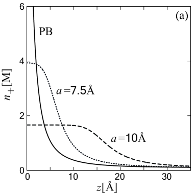
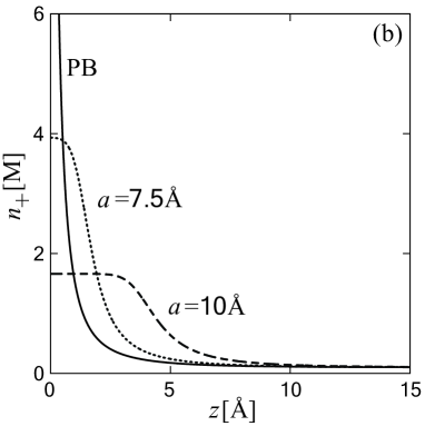
Figure 2: Counterions density profile calculated for the MPB model. The solid line represents the standard PB model, while the dotted and dashed lines represent the MPB results with molecular sizes of $7.5$Å and $10$Å, respectively. In (a) the salt is symmetric $1{:}1$, while in (b) it is asymmetric $1{:}4$. Other parameters are: $\sigma=-1/50\,$Å^-2, $n_{b}=0.1$M , and $\varepsilon=80$.

The local pressure $P_{\rm MPB}$ can be calculated with analogy to $P_{\rm PB}$ of (9)

$$P_{\rm MPB} = -\frac{\varepsilon}{8\pi}\psi^{\prime 2}+$$ (19t)

$$\frac{k_{\mathrm{B}}T}{a^{3}}\ln\left[1+\frac{1}{z_{+}+z_{-}}\frac{\hat{n}}{1-\hat{n}}\left(z_{-}\rme^{-ez_{+}\psi/k_{\mathrm{B}}T}+z_{+}\rme^{ez_{-}\psi/k_{\mathrm{B}}T}\right)\right]$$

and can be cast into the form of the contact theorem that relates the value of the equilibrium osmotic pressure to the values of the surface potential and its first derivative, yielding a generalization of the standard Graham equation used in the colloid science [12]

$$\sigma^{2}\simeq\frac{\varepsilon k_{\mathrm{B}}T}{2\pi}\frac{1}{a^{3}}\ln{\frac{1-2a^{3}n_{b}}{1-a^{3}n_{+}^{s}}}$$ (19u)

This analytical expression is valid in the limit that the co-ions have a negligible concentration at the surface, $n_{-}^{s}\to 0$. It is instructive to find that for $a\to 0$, expanding the logarithm in (19u), we recover the Graham equation for the standard PB model (10).

4 PB and charge regulation in lamellar systems

4.1 The model free energy and osmotic pressure

In the previous sections the surface free energy $F_{s}$ (6) was taken in its simplest form assuming a homogeneous surface charge, i.e. in the form of a surface electrostatic energy. We consider now a generalized form of $F_{s}$ where lateral mixing of charged species is allowed within the surface and is described on the level of regular solution theory [19].

Experimentally observed lamellar-lamellar phase transitions in charged surfactant systems [21] provides an example where non-electrostatic, ionic-specific interactions appear to play a fundamental role. The non-electrostatic interactions are limited to charged amphiphilic surfaces confining the ionic solution. As evidenced in NMR experiments, ions not only associate differently with the amphiphile-water interface, but their binding may also restructure the interface they contact [22]. Computer simulations also indicate that the restructuring of the amphiphilic headgroup region should be strongly influenced by the size of the counter-ion [23]. Such conformational changes at the interface are possible sources of non-ideal amphiphile mixing, because non-electrostatic ion binding at the interface may effectively create two incompatible types of amphiphiles: ion-bound and ion-detached.

We proposed a model [24] based on an extension of the Poisson–Boltzmann theory to explain the first-order liquid-liquid (${\rm L}_{\alpha}\rightarrow{\rm L}_{\alpha^{\prime}}$) phase transition observed in osmotic pressure measurements of certain charged lamellae-forming amphiphiles [21]. Our starting point is the same as depicted in figure 1. The free energy of the confined ions has several contributions. The volume free energy, $F_{\rm PB}$, is taken to be the same as the PB expression for the counterion only case (12). Because all counterions in solution originate from surfactant molecules, their integrated concentration (per unit area) must be equal in magnitude and opposite in sign to the surface charge density

$$2\sigma=e\int^{D/2}_{-D/2}n(z)\,{d}z$$ (19v)

This is also the electroneutrality condition and can be translated via Gauss’ law into the electrostatic boundary condition (in Gaussian units): $\psi^{\prime}(D/2)=\psi^{\prime}_{s}=4\pi\sigma/\varepsilon$, linking the surface electric field $\psi^{\prime}_{s}$ with the surface charge density $\sigma$.

The second part of the total free energy comes from the surface free energy, $F_{s}$, of the amphiphiles residing on the planar bilayers. Here, we deviate from the $F_{s}$ expression in (6) because we allow the surfactants on the interface to partially dissociate their counterion in the spirit of the Ninham-Parsegian theory of charge regulation [11]. The surface free energy $F_{s}$ has electrostatic and non-electrostatic parts as well as a lateral mixing entropy contribution. Expressed in terms of the dimensionless surface area fraction $\eta_{s}=a^{2}\sigma/e$ of charged surfactants and dimensionless surface potential $\Psi_{s}=e\psi_{s}/k_{\mathrm{B}}T$, the free energy $F_{s}$ is:

$$F_{s} = \frac{k_{\mathrm{B}}T}{a^{2}}\int_{\rm A}\mathrm{d}^{2}r\,\left[\eta_{s}\Psi_{s}-{\alpha_{s}}\eta_{s}-\frac{1}{2}{\chi_{s}}\eta_{s}^{2}\right.$$

$$+ \eta_{s}\ln\eta_{s}+(1-\eta_{s})\ln(1-\eta_{s})\Bigg{]}$$ (19w)

The first term couples the surface charge and surface potential as in (6), while the additional terms are the enthalpy and entropy of a two-component liquid mixture: charged surfactant with area fraction $\eta_{s}$ and neutralized, ion-bound surfactants with area fraction $1-\eta_{s}$. The dimensionless parameters ${\alpha_{s}}$ and ${\chi_{s}}$ are phenomenological, and denote respectively the counterion–surfactant and the surfactant–surfactant interactions at the surface. Here, ${\alpha_{s}}<0$ means that there is an added non-electrostatic attraction (favorable adsorption free energy) between counterions and the surface; the more counterions are associated at the surface, the smaller the amount of remaining charged surfactant. A positive ${\chi_{s}}$ parameter represents the tendency of surfactants on the surface to phase separate into domains of neutral and charged surfactants.

The total free energy $F_{\rm tot}$ is written as a functional of the variables $\Psi(z)$, $n(z)$, and a function of $\eta_{s}$, and includes the conservation condition, (19v), via a Lagrange multiplier, $\lambda_{s}$:

$$F_{\rm tot}[\Psi,n;\eta_{s}]=F_{\rm PB}+F_{s}-\lambda_{s}\left[\eta_{s}-{a^{2}}\int_{0}^{D/2}n(z)\,{\rm d}z\right]$$ (19x)

Next, we minimize $F_{\rm tot}$ with respect to the surface variable $\eta_{s}$, and the two continuous fields $n(z)$, $\Psi(z)$:  $\mathrm{d}F_{\rm tot}/\mathrm{d}\eta_{s}=\delta F_{\rm tot}/\delta n(z)=\delta F_{\rm tot}/\delta\Psi(z)=0,$ corresponding to three coupled Euler-Lagrange (EL) equations. The first one connects the surface charge density ${\eta_{s}}$ with the surface potential $\Psi_{s}$

$$\frac{\eta_{s}}{1-\eta_{s}} = \exp\left(\lambda_{s}+\alpha_{s}+\chi_{s}\eta_{s}-\Psi_{s}\right)$$ (19ya)

The second one is simply the Boltzmann distribution for the spatially–dependent ion density

$$a^{3}n(z) = \exp\left(-\lambda_{s}+\Psi(z)\right)$$ (19yb)

and the last one is the standard Poisson equation

$$\Psi^{\prime\prime}(z) = {4\pi l_{\mathrm{B}}n(z)}$$ (19yc)

In addition, the variation with respect to $\Psi_{s}$ gives the usual electrostatic boundary condition of the form

$$\Psi^{\prime}(D/2)=\Psi_{s}^{\prime}=\frac{4\pi l_{\mathrm{B}}\eta_{s}}{a^{2}}$$ (19yz)

The Lagrange multiplier, $\lambda_{s}$, acts as a chemical potential with the important difference that it is not related to any bulk reservoir, but rather to the concentration at the midplane, $n(0)$.

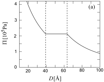
Figure 3: (a) The osmotic pressure $\Pi$ in units of $10^{5}$ Pascals; and, (b) the area fraction $\eta_{s}=a^{2}\sigma/e$ of surface charges, as function of inter-lamellar spacing $D$ for $\alpha_{s}=-6$, $\chi_{s}=12$ and $a=8$ Å. The Maxwell construction gives a coexistence between a phase with $D\simeq 39$ Å and low $\eta_{s}\leq 0.1$, and another with $D\simeq 64$ Å and $\eta_{s}\lesssim 1$. In (b) the two coexisting phases are denoted by squares and the dotted-dashed line shows the tie-line in the coexisting region.

Figure 4: Fit to the experimental osmotic pressure isotherm $\Pi(D)$ of Ref. [21] on a log-log scale. The diamonds and squares are the data points for DDABr and DDACl, respectively, reproduced from Ref. [21]. The solid line is the best fit of the model to the phase transition seen for DDABr with $\alpha_{s}=-7.4$, $\chi_{s}=14.75$ and $a=8$ Å. The fit also includes a hydration contribution (parameters for the form: $\Pi_{\rm hyd}=\Pi_{0}\exp(-D/\lambda_{\rm hyd})$, with typical values: $\Pi_{0}=2.37\cdot 10^{8}$ Pa and $\lambda_{\rm hyd}=1.51$ Å). This contribution is particularly important at the low $D$ region of the DDABr isotherm. A small amount of salt is added in the fits in the experiment ($n_{b}=0.5$ mM). The dashed line is the fit to the DDACl (no transition) and all parameters are the same as for the solid line, except $\alpha_{s}=-3.4$.

The non-electrostatic, ion-specific surface interactions govern the surface charged surfactant area fraction $\eta_{s}$, and has the form of a Langmuir-Frumkin-Davis adsorption isotherm [25]. Combining (19yb) and (19yc) together is equivalent to the PB equation. Their solution, together with the adsorption isotherm (19ya), completely determines the counterion density profile $n(z)$, the mean electrostatic potential $\Psi(z)$, and yields the osmotic pressure $\Pi$. We will apply this formalism to a specific example of lamellar-lamellar phase transitions next [24].

4.2 The lamellar-lamellar transition in amphiphilic systems

The typical isotherm $\Pi(D)$ shown in figure 3a exhibits a first-order phase transition from one free energy branch at large inter-lamellar separation $D$ to another at smaller $D$ — with a coexistence region in between. For given values of $\alpha_{s}$ and $\chi_{s}$ (chosen in the figure to be $\alpha_{s}=-6$ and $\chi_{s}=12$), and for large enough $D$ ($D\geq 64$Å), most counterions are dissociated from surfaces, $\eta_{s}\lesssim 1$, and the osmotic pressure follows the standard PB theory for (almost) fully dissociated surfactants. For smaller values of $D$ ($D<39$Å), most counterions bind to the surface $\eta_{s}\leq 0.1$ and the isotherm follows another branch, characterized by a much smaller surface charge of only about $10\%$ of the fully dissociated value. In intermediate $D$ range ($39{\rm\AA}\leq D\leq 64$Å), the system is in a two-phase coexistence, the osmotic pressure $\Pi$ has a plateau and $\eta_{s}$ changes from one branch to the second (figure 3b).

Our model is motivated by experiments [21] on the surfactant homolog series: DDACl, DDABr and DDAI The main experimental observation is reproduced in figure 4 along with our model fittings. When Cl^- serves as the counterion, as in DDACl, the osmotic pressure isotherm $\Pi(D)$ follows the usual PB result. When Br^- is the counterion, as in DDABr, one clearly observes a lamellar-lamellar phase transition from large inter-lamellar spacing of 60Åto small inter-lamellar spacings of about 10Å. In addition, for the largest counterion, I^-, as in DDAI, the lamellar stack cannot be swollen to the large $D$ values branch . We can fit the experimental data by assigning different $\alpha_{s}$ and $\chi_{s}$ values to the three homolog surfactants as can be seen in figure 4. Qualitatively, the different lamellar behavior can be understood in the following way. The Cl^- counterion is always dissociated from the DDA⁺ surfactant resulting in a PB-like behavior, and a continuous $\Pi(D)$ isotherm. For the Br^- counterion, the dissociation is partial as is explained above (figure 3) leading to a first-order transition in the isotherm and coexistence between thin and thick lamellar phases. Finally, for the DDAI, the I^- ion stays associated with the DDA⁺ surfactant and there is no repulsive interaction to stabilize the swelling of the stack for any $\Pi$ value. More details about our model and the fit can be found in [24].

Non-electrostatic interactions between counterion-associated and dissociated surfactants can be responsible for an inplane transition, which, in turn, is coupled to the bulk transition in the interaction osmotic pressure as can be clearly seen in figure 3. This proposed ion-specific interactions are represented in our model by $\chi_{s}$ and $\alpha_{s}$. While at present direct experimental verification and estimates for the proper $\chi_{s}$ values are lacking, the conformational changes induced by the adsorbing ion, together with van der Waals interaction between adsorbed ions can lead to significant demixing. Furthermore, because larger ions are expected to perturb the surfactant-water interface to a larger extent, it is reasonable to expect that the value of $\chi_{s}$ will scale roughly with the strength of surface-ion interactions, $\alpha_{s}$.

We note that the $\chi_{s}$ values needed to observe a phase transition, typically $\approx 10$ (in units of $k_{\mathrm{B}}T$), are quite high . These high values are needed to overcome the electrostatic repulsion between like-charged amphiphiles, leading to segregation. The source of this demixing energy, as codified by $\chi_{s}$, could be associated with mismatch of the hydrocarbon regions as well as headgroup-headgroup interactions, such as hydrogen bonding between neutral lipids, or indeed interactions between lipids across two apposed bilayers.

5 Mixed solvents effects in ionic solutions

So far, in most theoretical studies of interactions between charged macromolecular surfaces, the surrounding liquid solution was regarded as a homogeneous structureless dielectric medium within the so-called “primitive model”. However, in recent experimental studies on osmotic pressure in solutions composed of two solvents (binary mixture), the osmotic pressure was found to be affected by the binary solvent composition [26]. It thus seems appropriate to generalize the PB approach of section 2 by adding local solvent composition terms to the free energy.

Our approach is to generalize the bulk free energy terms to include regular solution theory terms for the binary mixture, augmented by the non-electrostatic interactions between ions and the two solvents in order to account adequately for the preferential solvation effects [27]. In this generalized PB framework the mixture relative composition will create permeability inhomogeneity that will be incorporated into the electrostatic interactions.

More specifically, our model consists of ions that are immersed in a binary solvent mixture confined between two planar charged interfaces. Note that the two surfaces are taken as homogeneous charge surfaces with negative surface charge $\sigma<0$. We do this to make contact with experiments on DNA that is also negatively charged [26]. Though the model is formulated on a mean-field level it upgrades the regular PB theory in two important aspects. First, the volume fractions of the two solvents, $\phi_{\mathrm{A}}$ and $\phi_{\mathrm{B}}=1-\phi_{\mathrm{A}}$, are allowed to vary spatially. Consequently, the dielectric permeability of the binary mixture is also a function of the spatial coordinates. In the following, we assume that the local dielectric response $\varepsilon(\mathbf{r})$ is a (linear) compositionally weighted average of the two permeabilities $\varepsilon_{\mathrm{A}}$ and $\varepsilon_{\mathrm{B}}$:

$$\varepsilon(\mathbf{r})=\phi_{\mathrm{A}}(\mathbf{r})\varepsilon_{\mathrm{A}}+\phi_{\mathrm{B}}(\mathbf{r})\varepsilon_{\mathrm{B}}\,,$$ (19yaa)

or,

$$\varepsilon(\mathbf{r})=\varepsilon_{0}-\phi(\mathbf{r})\varepsilon_{\mathrm{r}}\,,$$ (19yab)

where we define $\phi\equiv\phi_{\mathrm{B}}$, $\varepsilon_{0}\equiv\varepsilon_{\mathrm{A}}$ and $\varepsilon_{\mathrm{r}}\equiv\varepsilon_{\mathrm{A}}-\varepsilon_{\mathrm{B}}$. This linear interpolation assumption is not only commonly used but is also supported by experimental evidence [28]. Note that the incompressibility condition satisfies $\phi_{\mathrm{A}}+\phi_{\mathrm{B}}=1\,$, meaning that ionic volume fractions are neglected.

The second important modification to the regular PB theory is the non-electrostatic short-range interactions between ions and solvents. Those are mostly pronounced at small distances and lead to a reduction in the osmotic pressure for macromolecular separations of the order 10-20 Å. Furthermore, it leads to a depletion of one of the two solvents from the charged macromolecules (modeled here as planar interfaces), consistent with experimental results on the osmotic pressure of DNA solutions [26].

The model is based on the following decomposition of the free energy

$$F=F_{\rm PB}+F_{\rm mix}+F_{\rm sol}.$$

The first term, $F_{\rm PB}$ is the PB free energy of a 1:1 monovalent electrolyte as in (1) with one important modification. Instead of a homogeneous permeability, $\varepsilon$, representing a homogeneous solution, we will use a spatial-dependent dielectric function $\varepsilon(\mathbf{r})$ for the binary liquid mixture. The second term, $F_{\rm mix}[\phi]$, accounts for the free energy of mixing given by regular solution theory:

$$F_{\rm mix}=\frac{k_{\mathrm{B}}T}{a^{3}}\int\mathrm{d}^{3}r\,\left[\phi\ln\phi+(1-\phi)\ln(1-\phi)+\chi\phi(1-\phi)-\frac{\mu_{\phi}}{k_{\mathrm{B}}T}\phi\right]$$ (19yac)

The interaction parameter, $\chi$, is dimensionless (rescaled by $k_{\mathrm{B}}T$). As the system is in contact with a bulk reservoir, the relative composition $\phi$ has a chemical potential $\mu_{\rm\phi}$ which is determined by the bulk composition $\phi_{b}$. For simplicity, we take the same molecular volume $\sim a^{3}$ for both A and B components.

The third term, $F_{\rm sol}$, originates from the preferential non-electrostatic interaction of the ions with one of the two solvents. We assume that this preference can be described by a bilinear coupling between the ion densities, $n_{\pm}$, and the relative solvent composition $\phi$. This is the lowest order term that accounts for these interactions. The preferential solvation energy, $F_{\rm sol}$, is then given by

$$F_{\rm sol}=k_{\mathrm{B}}T\int\mathrm{d}^{3}r\,\left(\alpha_{+}n_{+}+\alpha_{-}n_{-}\right)\phi$$ (19yad)

where the dimensionless parameters $\alpha_{\pm}$ describe the solvation preference of the ions, defined as the difference between the solute (free) energies dissolved in the A and B solvents. Finally, to all these bulk terms one must add a surface term, $F_{s}$, [as in (6)] describing the electrostatic interactions between charged solutes and confining charged interfaces.

In thermodynamic equilibrium, the spatial profile of the various degrees of freedom characterizing the system is again obtained by deriving the appropriate Euler-Lagrange (EL) equations via a variational principle. The EL equations are then reduced to four coupled differential equations for the four degrees of freedom, $\psi(\mathbf{r})$, $n_{\pm}(\mathbf{r})$ and $\phi(\mathbf{r})$. First we have the Poisson equation

$${\bf\nabla}\cdot\left(\frac{\varepsilon}{4\pi}{\bf\nabla}\psi\right)+e(n_{+}-n_{-})=0$$ (19yaea)

then the Boltzmann distribution

$$\pm\frac{e\psi}{k_{\mathrm{B}}T}+\ln(n_{\pm}a^{3})+\alpha_{\pm}\phi-\mu_{\pm}=0$$ (19yaeb)

and finally the EL equation for the density field $$\phi(\mathbf{r})$$

$$\ln\left(\frac{\phi}{1-\phi}\right) + \frac{\varepsilon_{\mathrm{r}}a^{3}}{8\pi k_{\mathrm{B}}T}({\bf\nabla}\psi)^{2}+\chi(1-2\phi)$$ (19yaec)

$$+~{} a^{3}\left(\alpha_{+}n_{+}+\alpha_{-}n_{-}\right)-\frac{\mu_{\phi}}{k_{\mathrm{B}}T}=0$$

At the charged interface, the electrostatic boundary condition stems from the variation of $F_{s}$ with the difference that $\varepsilon(\phi)$ has a surface value: $\varepsilon_{s}=\varepsilon_{0}-\varepsilon_{\mathrm{r}}\phi_{s}$, so that the boundary condition becomes

$$\hat{{\bf n}}\cdot{\bf\nabla}\psi\bigg{|}_{s}=-\frac{4\pi e}{\varepsilon_{s}}\sigma,$$ (19yaeaf)

Again the boundary condition states the electroneutrality condition of the system as can be shown by the integral form of Gauss’ law.

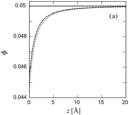
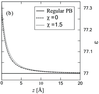
Figure 5: Spatial profiles of (a) the solvent relative composition $\phi$ and (b) the permeability $\varepsilon$. The regular PB with homogeneous dielectric constant $\varepsilon=77$ (solid line) is compared with our modified PB for binary mixture with and without short-range interactions, $\chi=0$ (dashed line) and $\chi=1.5$ (dotted line), respectively. Other parameters are: $\sigma=-1/100$Å^-2, $n_{\rm b}=10^{-4}$M, $\varepsilon_{\mathrm{A}}=80$, $\varepsilon_{\mathrm{B}}=20$ and $\phi_{\rm b}=0.05$. In all the cases, no preferential solvation is considered, $\alpha_{\pm}=0$.

By solving the above set of equations, one can obtain the spatial profiles of the various degrees of freedom at thermodynamic equilibrium. For a general geometry, these equations can be solved only numerically to obtain spatial profiles for $\phi$ and $n_{\pm}$. The osmotic pressure can then be evaluated via an application of the first integral of (19yaea), (19yaeb), (19yaec).This pressure is a function of the inter-plate separation $D$ and the experimentally controlled parameters $\alpha_{+}$, $\phi_{b}$ and $n_{b}$.

For two identically charged planar surfaces, in the absence of preferential solvation, the numerical solutions of the EL equations show (see figure 5) that the density profiles and, therefore, the osmotic pressure undergo only small modifications. By adding the preferential solvation term as quantified by $\alpha_{+}$, one observes a considerable correction to both the density profile, as well as the pressure (see figure 6). Most notably is the reduction in the osmotic pressure at small separations (10-20 Å) due to the coupling between ion density and solvent local composition.

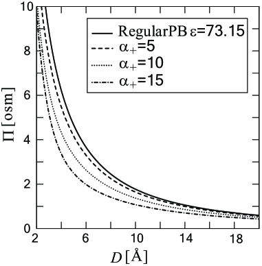
Figure 6: The dependence of pressure on separation $D$ for various ion-solvent interaction strengths $\alpha_{+}$. Other parameters are: $\sigma=-1/100$Å^-2, $n_{\rm b}=10^{-4}$M, $\varepsilon_{\mathrm{A}}=80$, $\varepsilon_{\mathrm{B}}=4$ and $\phi_{b}=0.09$.

6 Polarizable ions in solution

Ion-specific effects as manifested through the Hofmeister series have been recently associated with ionic polarizability, especially in the way they affect van der Wails electrodynamic interactions between ions and bounding interfaces [29]. However, this does not provide the full description, since the ionic polarizability also modifies the electrostatic interactions of ions with the surface charges.

In what follows we generalize the PB theory in order to include also the contribution of the ionic polarizability to the overall electrostatic interactions. This inclusion leads to a new model that again supersedes the standard PB theory. Note, that in a more complete and consistent treatment, the polarizability should also be taken into account in the electrodynamic van der Wails interactions, in addition to what we propose here.

We begin along the lines of section 5, while delimiting ourselves to the counterion polarizability in the electrostatic part of the free energy. In order to discuss a manageable set of parameters, we discard other possible non-electrostatic terms in the total free energy and concentrate exclusively on the changes brought about in the ionic density profile and the interaction osmotic pressure.

The free energy has the same form as $F_{\rm PB}$ for counterion only case (12) with one important difference that $\varepsilon=\varepsilon(n)$ is now a function of the counterion density $n$

$$F/A=\int\mathrm{d}z\left[-\frac{\varepsilon(n)}{8\pi}\psi^{\prime 2}+en\psi+k_{\mathrm{B}}Tn(\ln n-1)-\mu n\right]$$ (19yaeag)

The equilibrium equations read

$$\frac{\delta F}{\delta\psi}=4\pi en+\frac{\mathrm{d}}{\mathrm{d}z}\left[\varepsilon(n)\psi^{\prime}\right]=0$$ (19yaeaha)

$$\frac{\delta F}{\delta n}=-\frac{1}{8\pi}\frac{\partial\varepsilon(n)}{\partial n}\psi^{\prime 2}+e\psi+k_{\mathrm{B}}T\ln n=\mu$$ (19yaeahb)

The first equation is a generalization of the Poisson equation and the second is a generalization of the Boltzmann distribution. For the free energy (19yaeag) we can use the general first integral of the system that gives the pressure in the form:

$$P=-\frac{1}{8\pi}\left(\varepsilon(n)+\frac{\partial\varepsilon(n)}{\partial n}n\right)\psi^{\prime 2}+k_{\mathrm{B}}Tn$$ (19yaeai)

The first term is an appropriately modified form of the Maxwell stress tensor while the second one is the standard van ’t Hoff term.

¿From the first integral we furthermore derive the following relation:

$$\psi^{\prime}=\sqrt{\frac{8\pi k_{\mathrm{B}}T(n-\tilde{P})}{\varepsilon(n)+\frac{\partial\varepsilon(n)}{\partial n}n}}$$ (19yaeaj)

where $\tilde{P}=P/k_{\mathrm{B}}T$ is the rescaled pressure. Substituting this relation in (19yaeaha), we end up with a first-order ordinary differential equation for the ion density $n$:

$$\frac{\mathrm{d}n}{\mathrm{d}z}=-\sqrt{\frac{2\pi e^{2}}{k_{\mathrm{B}}T}}\frac{n}{{\partial f(n)}/{\partial n}}$$ (19yaeak)

where

$$f(n)=\varepsilon(n)\sqrt{\frac{n-\tilde{P}}{\varepsilon(n)+\frac{\partial\varepsilon(n)}{\partial n}n}}$$ (19yaeal)

is a function of the variable $n$ only. Equation (19yaeak) can be integrated explicitly either analytically or numerically, depending on the form of $f(n)$. Note that in thermodynamic equilibrium, the total osmotic pressure $P$ is a constant.

The boundary condition for a constant surface charge is given by

$$\varepsilon(n_{\rm s})\psi^{\prime}\big{|}_{\rm s}=4\pi e|\sigma|$$ (19yaeam)

where $\varepsilon(n_{s})$ and $n_{s}$ are the surface values of the dielectric function and ion density, respectively. Using the pressure definition, we arrive at an algebraic equation for the surface ion density:

$$n_{\rm s}-\tilde{P}=\frac{2\pi e^{2}\sigma^{2}}{k_{\mathrm{B}}T\varepsilon^{2}(n_{\rm s})}\left({\varepsilon(n_{\rm s})+\frac{\partial\varepsilon(n_{\rm s})}{\partial n_{\rm s}}n_{\rm s}}\right)$$ (19yaean)

For a single surface the pressure vanishes $\tilde{P}=0$ (with analogy to two surfaces at infinite separation, $D\to\infty$), and the basic equations simplify considerably.

As a consistency check, we take the regular case, i.e. a single charged surface with a homogeneous dielectric constant. In this case the function $f(n)$ takes the form $f(n)=\sqrt{\varepsilon_{0}n}$, and (19yaeak) reads:

$$\frac{\mathrm{d}n}{\mathrm{d}z}=-\sqrt{8\pi\l_{\rm B}}n^{\frac{3}{2}}$$ (19yaeao)

which gives the well known Gouy-Chapman result for the counter-ion profile close to a single charged plate (in absence of added salt) :

$$n(z)=\frac{1}{2\pi l_{\mathrm{B}}(z+\lambda_{\mathrm{GC}})^{2}}$$ (19yaeap)

where $\lambda_{\mathrm{GC}}=1/(2\pi l_{\mathrm{B}}|\sigma|)$ is the Gouy-Chapman length, found by satisfying the boundary condition (19yaeam)

We assume that to lowest order the dielectric constant can be expanded as a function of the counterion concentration $n$ as:

$$\varepsilon(n)=\varepsilon_{0}+\beta n+{\cal O}(n^{2}),$$ (19yaeaq)

where $\varepsilon_{0}$ is the dielectric constant of the solvent and $\beta={\partial\varepsilon}/{\partial n}|_{0}$ is a system parameter describing the molecular polarizability of the counterions in the dilute counterion limit.

The derivative of $f(n)$ to be used in (19yaeak) reads:

$$\frac{\partial f}{\partial n}=\frac{2\beta^{2}n(n-\tilde{P})+\varepsilon(n)[\varepsilon(n)+\beta n]}{2\sqrt{(n-\tilde{P})[\varepsilon(n)+\beta n]^{3}}}$$ (19yaear)

and (19yaeak) can now be solved explicitly for $n(z)$.

In figure 7 we show the spatial profile of the counterion density away from single charged surface. No extra salt is added and the pressure is zero $\tilde{P}=0$ for a single plate as mentioned above. In figure 7a we present the case where $\beta<0$ (i.e., the dielectric permeability in the regions of high ion density is smaller than in the pure solution). The ion density profile exhibits a somewhat “flat” behavior, indicating some saturation in the vicinity of the surface, while at a distances of $\sim 5\,$Å  and further away from the surface the density decays strongly to zero. In figure 7b the density profile is shown for the opposite case where $\beta>0$. Namely, when the dielectric permeability in the regions of high ion density is larger than in the pure solution. The profile here does not show large deviations from the usual Gouy-Chapman behavior even close to the surface.

Obviously, the effect of ionic polarizability strongly depends on the sign of the ionic polarizability, $\beta$. It appears that the dependence of the dielectric constant on ionic density introduces effective interactions between the ions and the bounding surface. For $\beta<0$, these additional interactions seem to be strongly repulsive and long ranged. They lead to a depletion of the ions in the vicinity of the surface. In the opposite case where for $\beta>0$, the interactions are also repulsive but extremely weak and the electric double layer structure remains almost unperturbed by the ionic polarization. This sets a strong criterion for ion specificity because the ions can be differentiated according to the sign of their polarizability affecting their surface attraction.

Figure 7: Ion density and permeability profiles. The solid lines in both panels represent the case where the ions have no contribution to the permeability, $\beta=0$, given by (19yaeap). In (a) the dashed line shows the ion density where their averaged permeability is smaller than the solution dielectric constant, $\beta=-30\,$M^-1. The permeability of the second case is shown in the inset. In (b) the dashed line shows the ion density where their averaged permeability is smaller than the solution dielectric constant, $\beta=20\,$M^-1. The permeability of the second case is shown in the inset. Other parameters in both (a) and (b) are: $\sigma=-1/100\,$Å^-2, and $\varepsilon_{0}=80$.

7 Conclusions

We presented here several attempts to generalize the PB theory by including in the free energy additional terms to the standard electrostatic and ideal entropy of mixing. We also showed how these terms lead to modifications of the PB equation and its boundary conditions. More specifically, we have aimed to include additional interactions between dissolved ions, such as finite ion size and polarizability, as well as their solvation and interactions with bounding surfaces. All these endeavors are done within the mean-field approximation while neglecting charge density fluctuations and ion correlations.

The approach presented here amends the free energy in specific ways giving rise to modified electric bilayer charge distribution and ensuing interactions between charged surfaces as mediated by ionic solutions. Some modification wrought by the non-electrostatic terms can be interpreted in retrospect as specific interactions of the ions with the bounding surfaces or between the ions themselves.

To verify these models, results should be compared with appropriate experiments. In some cases, such comparisons are feasible and are qualitatively favorable [24, 27]. On the other hand, comparisons with extensive all-atom MC or MD simulations are not obvious since these simulations also contain multiple parameters that have no obvious analogue. It would, nevertheless, be valuable to link these approaches with appropriately designed experiments or even to check the predictions of these approaches in realistic systems.

References

References

- [1] Poon W C K and Andelman D 2006 Soft Condensed Matter Physics in Molecular and Cell Biology, (Taylor & Francis).
- [2] Oosawa F 1968 Biopolymers 6 1633
- [3] Naji A, Jungblut S, Moreira A G and Netz R R 2005 Physica A 352 131
- [4] Boroudjerdi H, Kim Y W, Naji A, Netz R R, Schlagberger X and Serr A 2005 Phys. Rep. 416 129
- [5] Chan D Y C, Mitchell D J, Ninham B W and Pailthorpe B A 1979 in Water: A Comprehensive Treatise (Vol. 6 Recent Advances) Ed F Franks (New York: Plenum). Conway B E 1981 Ionic Hydration in Chemistry and Biophysics, (Studies in Physical & Theoretical Chemistry) (Amsterdam: Elsevier). Marcus Y 1997 Ion Properties, CRC; 1st edition. Leikin S, Parsegian V A, Rau D C and Rand R P 1993 Annu. Rev. Phys. Chem. 44 369. Ben-Naim A 1987 Solvation Thermodynamics (New York: Plenum)
- [6] Tanford C 1980 The Hydrophobic Effect: Formation of Micelles & Biological Membranes, (Wiley, New York). Chandler D 2005 Nature 437 640. Meyer E E, Rosenberg K J and Israelachvili J 2006 PNAS 103 15739. Dill K A, Truskett T M, Vlachy V and Hribar-Lee B 2005 Annu. Rev. Biophys. Biomol. Struct. 34 173
- [7] Marcus Y 2007 Chem. Rev. 107 3880. Kalidas C, Hefter G and Marcus Y 2000 Chem. Rev. 100 819
- [8] Vlachy N, Jagoda-Cwiklik B, Vácha R, Touraud D, Jungwirth P and Kunz W 2009 Adv. Coll. Interf. Sci. 146 42
- [9] Onuki A and Kitamura H 2004 J. Chem. Phys. 121 3143. Onuki A 2006 Phys. Rev. E 73 021506. Onuki A 2008 J. Chem. Phys. 128 224704. Tsori Y and Leibler L 2007 Proc. Natl. Acad. Sci. (USA) 104 7348
- [10] Hofmeister F 1888 Archiv. Exp. Path. Pharm. 24 247. Collins K and Washbaugh M 1985 Q. Rev. Biophys. 18 323. Harries D and Rösgen J 2008 Meth. Cell Biol. 84 679
- [11] Ninham B W and Parsegian V A 1971 J. Theor. Biol. 31 405. Chan D, Perram J W, White L R and Healy T H 1975 J. Chem. Soc., Faraday Trans. 1 71 1046. Chan D, Healy T and White L R 1976 ibid 72 2844. Prieve D C and Ruckenstein E 1976 J. Theor. Biol. 56 205. Pericet-Camara R, Papastavrou G, Behrens S H and Borkovec M 2004 J. Phys. Chem. B 108 19467. Von Grünberg H H 1999 J. Colloid Interface Sci. 219 339
- [12] Evans D F and Wennerstroem H 1994 The Colloidal Domain (Wiley-VCH)
- [13] Eigen M and Wicke E 1954 J. Phys. Chem. 58 702
- [14] Kralj-Iglic V and Iglic A 1996 J. Phys. II (France) 6 477
- [15] Borukhov I, Andelman D and Orland H 1997 Phys. Rev. Lett. 79 435. Borukhov I, Andelman D and Orland H 2000 Electrochim. Acta 46 221.
- [16] Tresset G 2008 Phys. Rev. E 78 061506
- [17] Israelachvili J N 1992 Intermolecular and Surface Forces (Elsevier)
- [18] Messina R 2009 J. Phys.: Condens. Matter 21 113102
- [19] Hill T L 1986 An Introduction to Statistical Theromodynamics (New York: Dover)
- [20] Stern O 1924 Z. Elektrochem. 30 508. Henderson D 1983 Prog. Surf. Sci. 13 197. Volkov A G, Deamer D W, Tanelian D L and Mirkin V S 1997 Prog. Surf. Sci. 53 1. Kjellander R and Marcelja S 1986 J. Phys. Chem. 90 1230. Kjellander R, Akesson T, Jonsson B and Marcelja S 1992 J. Chem. Phys. 97 1424
- [21] Dubois M, Zemb Th, Fuller N, Rand R P and Parsegian V A 1998 J. Chem. Phys. 108 7855
- [22] Rydall J R and Macdonald P M 1992 Biochemistry 31 1092
- [23] Sachs J N and Woolf T B 2003 J. Am. Chem. Soc. 125 874
- [24] Harries D, Podgornik R, Parsegian V A, Mar-Or E and Andelman D 2006 J. Chem. Phys. 124 224702
- [25] Davis J T 1958 Proc. Royal Soc. A 245 417
- [26] Stanely R and Rau D C 2006 Bipophys. J. 91 912
- [27] Ben-Yaakov D, Andelman D, Harries D and Podgornik R 2009 J. Phys. Chem. B 113 6001
- [28] Arakawa T and Timasheff S N, 1985 Methods Enzymol. 114 49
- [29] Ninham B W and Yaminsky V 1997 Langmuir 13 2097. Bostrom M, Williams D R M and Ninham B W 2001 Phys. Rev. Lett. 87 168103
- [30] Kunz W, Nostro P and Ninham B W 2004 Curr. Opin. Colloid Interf. Sci. 9 1
- [31] Kilic M S, Bazant M Z and Ajdari A 2007 Phys. Rev. E 75 021502
- [32] Garidel P, Johann C and Blume A 2000 J. Lip. Res. 10 131