On the maximization of a class of functionals on convex regions, and the characterization of the farthest convex set

Abstract

We consider a family of functionals $J$ to be maximized over the planar convex sets $K$ for which the perimeter and Steiner point have been fixed. Assuming that $J$ is the integral of a quadratic expression in the support function $h$, we show that the maximizer is always either a triangle or a line segment (which can be considered as a collapsed triangle). Among the concrete consequences of the main theorem is the fact that, given any convex body $K_{1}$ of finite perimeter, the set in the class we consider that is farthest away in the sense of the $L^{2}$ distance is always a line segment. We also prove the same property for the Hausdorff distance.

Keywords: isoperimetric problem, shape optimization, convex geometry, polygons, farthest convex set

AMS classification: 52A10, 52A40, 52B60, 49Q10

1 Introduction

Given a convex set $K_{1}$ in the plane, consider the problem of finding a second convex set that is as far as possible from $K_{1}$ in the sense of usual distances like the Hausdorff distance or the $L^{2}$ distance, subject to two natural geometric constraints, viz., that the two sets have the same perimeter and Steiner point, without either of which conditions there are sets arbitrarily far away from $K_{1}$. A plausible conjecture, which we prove below, is that the farthest convex set, subject to the two constraints, is always a “needle,” to use the colorful terminology of Pólya and Szegő [12] for a line segment in the plane.

In the case of the $L^{2}$ distance, the problem of the farthest convex set can be expressed as the maximization of a quadratic integral functional of the support function of the desired set, and, as we shall show, with the same two geometric constraints it is possible to characterize the maximizers of a wider class of such functionals as either triangles or needles, which, intuitively, can be considered as collapsed triangles. One of our inspirations for pursuing the wider class of functionals, the maximizers of which are triangles, is a recent article [8], in which the maximizers of another class of convex functionals were shown to be polygons. Now, the maximizers of a convex functional must lie on the boundary of the feasible set, which is to say, in our case or that of [8], that the maximizers will be nonstrictly convex, but not simple polygons a priori. What restrictions are needed on the functional to imply furthermore that the maximizer must be triangular? In this article, we consider functionals that are expressible as integrals of quadratic expressions in the support function, and show that the maximizers are always generalized triangles, i.e., triangles or needles.

An advantage of describing shape-optimization problems through the support function $h$ is that it is easy to express many geometric features, including perimeter and area, in terms of $h$. Yet another tool that is available to in the case of functionals that are quadratic in $h$ is that of Fourier series [3], because through the Parseval relation it is possible to rewrite many such functionals as series with geometric properties accessible through the form of the coefficients. Indeed another one of our inspirations was the analysis of the maximizers of the $L^{2}$ means of chord lengths of curves through Fourier series found in [2, 1]. When the means with respect to arc length are replaced with means weighted by curvature, the problem falls within the category of quadratic functionals of $h$ considered in this article. Interestingly, the cases of optimality of the weighted and unweighted problems are completely different. Because additional analysis is possible for quadratic functionals when the coefficients in the equivalent series enjoy certain properties, we shall defer details on the chord problem to a future article [5].

This paper is organized as follows: We begin Section 2 with the main notation and general optimality conditions. We state our main result in Subsection 2.3. Next, Section 3 is devoted to the problem of finding the farthest convex set. We begin with an inequality involving the minimum and the maximum of the support function, in the spirit of [10]. Then, we consider the case of the Hausdorff distance and we finish with the case of the $L^{2}$ distance, for which our main result is essential.

2 Notation and preliminary results

2.1 Notation

When convenient $\mathbb{R}^{2}$ will be identified with the complex plane, and the dot product of two vectors ${\bf x}$ and ${\bf w}$ with $\Re({x\,{\overline{w}}})$. Let $\mathbb{T}$ be the unit circle, identified with $[0,2\pi)$. For $\theta\in\mathbb{T}$, we will denote by $h_{K}(\theta)$ (or more simply $h(\theta)$ if not ambiguous) the support function of the convex set $K$; we recall that by definition $h(\theta)$ is the distance from the origin to the support line of $K$ having outward unit normal $e^{i\theta}$:

$$h_{K}(\theta):=\max\{x\cdot e^{i\theta}:x\in K\}\,.$$

It is known that the boundary of a planar convex set has at most a countable number of points of nondifferentiability. More precisely, the two directional derivatives of the function defining any portion of the boundary exist at every point and their difference is uniformly bounded. We refer to [13, 15] for this and other standard facts about convex regions. It follows from the regularity of the boundary that the support function $h$ belongs to the periodic Sobolev space $H^{1}(\mathbb{T})$.

For a polygon $K$ with $n$ sides, we let $a_{1},a_{2},\ldots,a_{n}$ and $\theta_{1},\theta_{2},\ldots,\theta_{n}$ denote the lengths of the sides and the angles of the corresponding outer normals. The following characterization of the support function of such a polygon is classical and will be useful here:

Proposition 2.1.

With the above notation, the support function of the polygon $K$ satisfies

$$\frac{d^{2}h_{K}}{d\theta^{2}}+h_{K}=\sum_{j=1}^{n}a_{j}\delta_{\theta_{j}}$$ (1)

where the derivative is to be understood in the sense of distributions and $\delta_{\theta_{j}}$ stands for a Dirac measure at point $\theta_{j}$.

Eq. (1) can be proved by a direct calculation. It is a special case of a formula of Weingarten, whereby for any support function $h_{K}$ of a convex set $K$, $\frac{d^{2}h_{K}}{d\theta^{2}}+h_{K}=h_{K}^{\prime\prime}+h_{K}$ is a nonnegative measure, which is interpreted as the (generalized) radius of curvature $R$ at the point of contact with the support line corresponding to $\theta$. We will denote by $S_{h}$ (or $S_{K}$ if we want to emphasize the dependence on the convex set $K$) the support of this measure. It will be useful to recover the support function from the radius of curvature. This can be accomplished by solving the ordinary differential equation:

$$h^{\prime\prime}+h=R$$ (2)

for a $2\pi$-periodic function $h(\theta)$ subject to the conditions

$$\int_{0}^{2\pi}h(\theta)\cos\theta\,d\theta=\int_{0}^{2\pi}h(\theta)\sin\theta\,d\theta=0\,.$$ (3)

These orthogonality conditions are imposed because (2) is in the second Fredholm alternative and hence needs such conditions for uniqueness. They can always be arranged by a choice of the origin, viz., that it is fixed at the Steiner point $s(K)$. Recall that the Steiner point $s(K)$ of a convex planar set $K$ is defined by

$$s(K)=\frac{1}{\pi}\int_{0}^{2\pi}h_{K}(\theta)e^{i\theta}\,d\theta\,.$$ (4)

By Fredholm’s condition for existence the function or measure $R(\theta)$ on the right side of (2) must satisfy the same orthogonality, that is,

$$\int_{0}^{2\pi}R\cos\theta\,d\theta=\int_{0}^{2\pi}R\sin\theta\,d\theta=0.$$

Since these restrictions on the radius of curvature are necessary conditions in any case for the closure of the boundary curve of $K$, they are automatically fulfilled.

An explicit Green function can be found to solve (2) for $h$ in terms of $R$, i.e., $G(t):=\frac{1}{2}\,\left(1-\frac{|t|}{\pi}\right)\sin|t|$, in terms of which

$$h(\theta)=\frac{1}{2}\int_{-\pi}^{\pi}G(t)R(\theta+t)\,dt\,.$$ (5)

The perimeter $P(K)$ of the convex set can be easily calculated from $h_{K}$:

$$P(K)=\int_{0}^{2\pi}h_{K}(\theta)\,d\theta\,.$$ (6)

In this article, we work within the class of convex sets whose Steiner point is at the origin and whose perimeter $P(K)$ is fixed, at a value that can be chosen as $2\pi$ without loss of generality:

$$\mathcal{A}:=\{K\;\mbox{convex set in }\mathbb{R}^{2},s(K)=O,P(K)=2\pi\}.$$ (7)

Given that convexity is equivalent to the nonnegativity of the radius of curvature $R=h^{\prime\prime}+h$ (in the sense of measures), the geometric set $\mathcal{A}$ can be described in analytic terms by requiring $h$ to lie in the function space:

$$\begin{array}[]{l}\mathcal{H}:=\{h\in H^{1}(\mathbb{T}),h\geq 0,\;h^{\prime\prime}+h\geq 0,\\ \quad\quad\int_{0}^{2\pi}hd\theta=2\pi,\;\int_{0}^{2\pi}h\cos\theta d\theta=\int_{0}^{2\pi}h\sin\theta d\theta=0\}.\end{array}$$ (8)

The class ${\mathcal{A}}$ contains in particular “needles,” i.e., line segments, which we regard as degenerate convex bodies in the sense that the perimeter of the segment is taken as twice its length. We shall let $\Sigma_{\alpha}$ designate the segment $[-i\frac{\pi}{2}e^{i\alpha},i\frac{\pi}{2}e^{i\alpha}]$. Its support function is given by

$$h_{\alpha}(\theta):=\frac{\pi}{2}|\sin(\theta-\alpha)|\,,$$ (9)

which satisfies ${h_{\alpha}}^{\prime\prime}+h_{\alpha}=\pi(\delta_{\alpha}+\delta_{\pi+\alpha})$.

2.2 Optimality conditions

If the goal is to maximize a functional $J$ defined on the geometric class ${\mathcal{A}}$, and $J$ is expressible in terms of the support function $h$, then we may equivalently consider the problem of determining

$$\max\{J(h):h\in\mathcal{H}\}.$$ (10)

We may then analytically determine the conditions for optimality of $J$.

The Steiner point $s$ of a closed convex set always lies within the set, and in the case of a convex body (a convex set of nonempty interior), $s$ is an interior point; see, e.g., (1.7.6) in [14]. It follows that the support function of $K$ can vanish only if $K$ is a segment. For any convex body in ${\mathcal{A}}$, $h_{K}(\theta)>0$ for all $\theta$.

We next derive the first and second order optimality conditions assuming that the optimal set is not a segment, following [8].

Theorem 2.2.

If $h_{0}>0$ is a solution of (10), where $J:H^{1}(\mathbb{T})\to\mathbb{R}$ is $C^{2}$, then there exist $\xi_{0}\in H^{1}(\mathbb{T})$, $\xi_{0}\leq 0$, and $\mu\in\mathbb{R}$ such that

$$\xi_{0}=0\;\mbox{on }S_{h_{0}},$$ (11)

and $\forall v\in H^{1}(\mathbb{T})$,

$$\left\langle{J^{\prime}(h_{0}),v}\right\rangle=\left\langle{\xi_{0}+{\xi_{0}}^{\prime\prime},v}\right\rangle+\mu\int_{0}^{2\pi}v\,d\theta\,.$$ (12)

Moreover, if $v\in H^{1}(\mathbb{T})$ such that $\exists\lambda\in\mathbb{R}$ satisfies

$$\begin{array}[]{l}v^{\prime\prime}+v\geq\lambda({h_{0}}^{\prime\prime}+h_{0})\\ v\geq\lambda h_{0}\\ \left\langle{\xi_{0}+{\xi_{0}}^{\prime\prime},v}\right\rangle+\mu\int_{0}^{2\pi}v\,d\theta=0.\end{array}$$ (13)

then

$$\left\langle{J^{\prime\prime}(h_{0}),v,v}\right\rangle\leq 0\,.$$ (14)

The proof of the foregoing theorem is classical and can be achieved using standard first and second order optimality conditions in infinite dimension space as in [11]; we refer to [8] for technical details.

Remark 1.

If the optimal domain $K_{0}$ is a segment, then the optimality condition is more complicated to write, because the constraint $h\geq 0$ needs to be taken into account. Since it will not be needed here, we do not write the explicit form.

2.3 Integral functionals

In this section, we are interested in quadratic functionals involving the support function and its first derivative. Let $J$ be the functional defined by:

$$J(K):=\int_{0}^{2\pi}{a\,h_{K}^{2}+b\,{h^{\prime}_{K}}^{2}+c\,h_{K}+d\,{h^{\prime}_{K}}\,d\theta},$$ (15)

where $a$ and $b$ are nonnegative bounded functions of $\theta$, one of them being positive almost everywhere on $\mathbb{T}$. The functions $c,d$ are assumed to be bounded. Our main theorem is the following:

Theorem 2.3.

Every local maximizer of the functional $J$ defined in (15), within the class ${\mathcal{A}}$ is either a line segment or a triangle.

Proof.

Let $K$ be a local maximizer of the functional $J$. We have to prove that the support $S_{K}$ of the measure $h_{K}^{\prime\prime}+h_{K}$ contains no more than three points. We follow ideas contained in [7] and [8].

Assume, for the purpose of a contradiction, that $S_{K}$ contains at least four points $\theta_{1}<\theta_{2}<\theta_{3}<\theta_{4}$ in $(0,2\pi)$. We solve the four differential equations

$$\left\{\begin{array}[]{l}v_{i}^{\prime\prime}+v_{i}=\delta_{\theta_{i}}\quad\theta\in(\theta_{1}-\varepsilon,\theta_{4}+\varepsilon)\\ v_{i}(\theta_{1}-\varepsilon)=v_{i}(\theta_{4}+\varepsilon)=0,\end{array}\right.$$ (16)

where $\delta_{\theta_{i}}$ is the Dirac measure at point $\theta_{i}$ and $\varepsilon>0$ is chosen such that $\theta_{4}+\varepsilon-(\theta_{1}-\varepsilon)<2\pi$. Note that equations (16) have unique solutions since we avoid the first eigenvalue of the interval. We also extend each function $v_{i}$ by 0 outside $(\theta_{1}-\varepsilon,\theta_{4}+\varepsilon)$. Now we can always find four numbers $\lambda_{i}$, $i=1,\ldots,4$ such that the three following conditions hold, where we denote by $v$ the function defined by $v=\sum_{i=1}^{4}\lambda_{i}v_{i}$:

$$v^{\prime}(\theta_{1}-\varepsilon)=v^{\prime}(\theta_{4}+\varepsilon)=0,\quad\int_{0}^{2\pi}v\,d\theta=0\,.$$ (17)

Then the function $v$ solves $v^{\prime\prime}+v=\sum_{i=1}^{4}\lambda_{i}\delta_{\theta_{i}}$ globally on $(0,2\pi)$. Now, we use the optimality conditions (11), (12) for the function $v$. We have

$$<\xi_{0}+{\xi_{0}}^{\prime\prime},v>+\mu\int_{0}^{2\pi}v\,d\theta=<v^{\prime\prime}+v,\xi_{0}>=\sum_{i=1}^{4}\lambda_{i}\xi_{0}(\theta_{i})=0\,.$$

Therefore, $v$ is admissible for the second order optimality condition (it is immediate to check that the two first conditions in (13) are satisfied by choosing $\lambda<0$ with $|\lambda|$ large enough). Since the functional $J$ is quadratic, however, this would imply $\int_{0}^{2\pi}a{v^{\prime}}^{2}+bv^{2}\,d\theta\leq 0$ which is impossible by the assumptions on $a$ and $b$. ∎

Remark 2.

The examples given in the next section may give the impression that the maximizers for such functionals are always segments. This is not the case. Indeed, if we choose $a=c=d=0$ and $b$ a (positive) function equal to one in a $\varepsilon$ neighborhood of $0,2\pi/3$ and $4\pi/3$ and very small elsewhere, the value for the equilateral triangle is of order $12\pi^{2}\varepsilon/27$ while the value for the best segment is of order $\pi^{2}\varepsilon/4$.

3 The farthest convex set

3.1 Introduction

There are many ways to define the distance between convex sets. Among them we single out the classical Hausdorff distance:

$$d_{H}(K,L):=\max\{\rho(K,L),\rho(L,K)\},$$

where $\rho$ is defined by

$$\rho(A,B):=\sup_{x\in A}\inf_{y\in B}|x-y|$$

(For a survey of possible metrics we refer to [4]; for a detailed study of the Hausdorff distance see [6]). It is remarkable that the Hausdorff distance can also be defined using the support functions, as $d_{H}(K,L)=\|h_{K}-h_{L}\|_{\infty}$. Moreover the support function allows a definition of the $L^{2}$ distance, introduced by McClure and Vitale in [9], by

$$d_{2}(K,L):=\left(\int_{0}^{2\pi}|h_{K}-h_{L}|^{2}\,d\theta\right)^{1/2}\,.$$

In [10], P. McMullen was able to determine the diameter in the sense of the Hausdorff distance of the class ${\mathcal{A}}$ in any dimension. More precisely, he proved that all sets in ${\mathcal{A}}$ are contained in the ball of radius $\pi/2$ centered at the origin. In terms of the support function, this means that, for any convex set $K$ in ${\mathcal{A}}$, the maximum of $h_{K}$ is at most $\pi/2$ (or $P(K)/4$). We will need the following more precise result:

Theorem 3.1.

Let $K$ be any plane convex set with its Steiner point at the origin. Then

$$\max h_{K}\leq\dfrac{P(K)}{4}\,\leq\min h_{K}+\max h_{K},$$ (18)

where both inequalities are sharp and saturated by any line segment.

Proof.

The first inequality in (18) is due to McMullen, who proved it in any dimension; see Theorem 1 in [10]. Let us prove the second inequality. Letting $B$ denote the unit ball, we introduce

$$\max h_{K}=\tau(K):=\min\{\tau>0/K\subset\tau B\}\,,$$

$$\min h_{K}=\rho(K):=\max\{\rho>0/\rho B\subset K\}\,.$$

The function $\tau(K)$ is convex with respect to the Minkowski sum, which can be defined with the support function via

$$h_{aK+bL}=ah_{K}+bh_{L}.$$

In contrast, the function $\rho(K)$ is concave, and as we are interested in the sum $F(K):=\tau(K)+\rho(K)$ we can call upon no particular convexity property. The minimum of $h_{K}$ is attained at some point we call $P$ and the maximum at some point $Q$ (see Figure 2). Let us denote by $L$ the line containing the points $O$ and $P$ and by $\sigma_{L}$ the reflection across $L$. If we replace the convex set $K$ by $\frac{1}{2}K+\frac{1}{2}\sigma_{L}(K)$, we keep the Steiner point at the origin, we preserve the perimeter, and we decrease $\tau$, because of convexity, without changing $\rho$. Therefore, to look for minimum of $F(K)$, we can restrict ourselves to convex sets symmetric with respect to the line $L$ passing through the point where $h_{K}$ attains its minimum. Now, let $S$ be the segment in the class ${\mathcal{A}}$ which is orthogonal to the line $L$.

We introduce the family of convex sets $K_{t}:=tK+(1-t)S$ and study the behavior of $t\mapsto F(K_{t})$. Since the ball $t\rho(K)B$ is included in $K_{t}$ and touches its boundary at $tP$, we have $\rho(K_{t})=t\rho(K)$. Moreover, by convexity $\tau(K_{t})\leq t\tau(K)+(1-t)\tau(S)$. Therefore, since $\tau(S)=F(S)$

$$F(K_{t})\leq tF(K)+(1-t)F(S)\,.$$ (19)

In particular, this imples that if $F(K)<F(S)$, we would also have $F(K_{t})<F(S)$ for $t$ near $0$. Thus, to prove the result it suffices to prove that a segment is a local minimizer for $J$. Without loss of generality, we consider the segment $\Sigma_{0}$ and perturbations respecting the symmetry with respect to the line $\theta=0$. Let us therefore consider a perturbation of the segment $\Sigma_{0}$, replacing its “radius of curvature” $R_{0}=\pi(\delta_{0}+\delta_{\pi})$ by

$$R_{t}=R_{0}+t[\varphi(x)-(\beta\delta_{0}+(1-\beta)\delta_{\pi})]$$

where $\varphi(x)$ is a non negative measure. Since we can work in the class of symmetric convex sets, we may assume $\varphi$ to be even. Moreover, we have to assume that $\int_{0}^{2\pi}R_{t}=2\pi$ and $\int_{0}^{2\pi}R_{t}\cos(\theta)=0$ (the last relation $\int_{0}^{2\pi}R_{t}\sin(\theta)=0$ is true by symmetry). This implies that

$$\begin{array}[]{c}\vspace{2mm}\int_{0}^{2\pi}\varphi=1,\quad\mbox{or}\quad\int_{0}^{\pi}\varphi=\frac{1}{2}\,,\\ \int_{0}^{2\pi}\varphi\cos\theta=2\beta-1,\quad\mbox{or}\quad\beta=\frac{1}{2}+\int_{0}^{\pi}\varphi\cos\theta\,.\end{array}$$ (20)

Now, the support function $h_{t}$ of the perturbed convex set can be obtained thanks to formulae (5):

$$h_{t}(\theta)=\frac{\pi}{2}|\sin\theta|+t\left\{\int_{-\pi}^{\pi}G(\tau)\varphi(\theta+\tau)\,d\tau-\beta G(\theta)-(1-\beta)G(\theta-\pi)\right\},$$

where $G$ denotes the Green function. The function $h_{t}$ will have its maximum near $\pi/2$, so to first order,

$$\max h_{t}=h_{t}(\frac{\pi}{2})+o(t)=\frac{\pi}{2}+t\left\{\int_{-\pi}^{\pi}G(\tau)\varphi(\tau+\frac{\pi}{2})\,d\tau-\frac{1}{2}\right\}+o(t)\,.$$ (21)

In the same way, the minimum of $h_{t}$ will be attained near $0$ or near $\pi$ so to first order

$$\begin{array}[]{l}\min h_{t}=\min(h_{t}(0),h_{t}(\pi))+o(t)=\\ \hskip 56.9055ptt\min\left\{\int_{-\pi}^{\pi}G(\tau)\varphi(\tau)\,d\tau,\int_{-\pi}^{\pi}G(\tau)\varphi(\tau+\pi)\,d\tau\right\}+o(t)\,.\end{array}$$ (22)

Therefore, we have to prove that

$$\int_{-\pi}^{\pi}G(\tau)\varphi(\tau+\frac{\pi}{2})\,d\tau+\int_{-\pi}^{\pi}G(\tau)\varphi(\tau)\,d\tau-\frac{1}{2}>0$$ (23)

and

$$\int_{-\pi}^{\pi}G(\tau)\varphi(\tau+\frac{\pi}{2})\,d\tau+\int_{-\pi}^{\pi}G(\tau)\varphi(\tau+\pi)\,d\tau-\frac{1}{2}>0\,.$$ (24)

Let us prove for example (23); the other inequality is similar. Letting

$$A:=\int_{-\pi}^{\pi}G(\tau)\varphi(\tau+\frac{\pi}{2})\,d\tau+\int_{-\pi}^{\pi}G(\tau)\varphi(\tau)\,d\tau=\int_{-\pi}^{\pi}(G(\tau)+G(\tau-\frac{\pi}{2}))\varphi(\tau)\,d\tau$$

and using the fact that $\varphi$ is even,

$$A=\int_{0}^{\pi}[G(\tau)+G(\tau-\frac{\pi}{2})+G(-\tau)+G(-\tau-\frac{\pi}{2})]\varphi(\tau)\,d\tau\,.$$

Now, it is elementary to check that the function $\tau\mapsto G_{4}(\tau):=G(\tau)+G(\tau-\frac{\pi}{2})+G(-\tau)+G(-\tau-\frac{\pi}{2})$ is always greater or equal to one (see Figure 1)

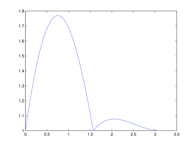
Figure 1: The function $\tau\mapsto G(\tau)+G(\tau-\frac{\pi}{2})+G(-\tau)+G(-\tau-\frac{\pi}{2}$).

so we have $A\geq\int_{0}^{\pi}\varphi(\tau)\,d\tau=\frac{1}{2}$. Moreover, since the function $G_{4}$ is equal to one only for $\tau=0,\pi/2$ or $\pi$, the inequality will be strict unless the support of $\varphi$ is concentrated at the four points $-\pi/2,0,\pi/2,\pi$. This last case actually corresponds to a (thin) rectangle $K_{\alpha}=[-\alpha,\alpha]\times[-\pi/2+\alpha,\pi/2-\alpha]$ for which a direct computation shows that $\min h_{K_{\alpha}}=\alpha/2$ and $\max h_{K_{\alpha}}=\left(\alpha^{2}+(\pi-\alpha)^{2}\right)^{1/2}/2$, and $F(K_{\alpha})>\pi/2=F(S)$ follows immediately. ∎

Another consequence of McMullen’s result cited above is that the Hausdorff distance between two sets in ${\mathcal{A}}$ is always less or equal to $\pi/2$, the upper bound being obtained by two orthogonal segments.

In this section, we want to deal with a similar question, namely to find the farthest convex set in the class ${\mathcal{A}}$ from a given convex set, as measured by either of the two distances defined above. More precisely, letting $C$ be a given convex set in the class ${\mathcal{A}}$, we wish to find the convex set $K_{C}$ such that

$$d(C,K_{C})=\max\{d(C,K):K\in{\mathcal{A}}\},$$

where $d$ may stand either for $d_{H}$ or for $d_{2}$.

First of all, let us give an existence result for such a problem.

Theorem 3.2.

Let $d(.,.)$ be a distance function for convex sets that behaves continuously under uniform convergence of the support functions. Then the problem

$$\max\{d(C,K):K\in{\mathcal{A}}\}$$ (25)

has a solution.

Proof.

For the proof we will use the following Lemma:

Lemma 3.3.

For any $h$ in the set ${\mathcal{H}}$ (defined in (8)), we have

$$\|h\|^{2}_{H^{1}}\leq 16\pi/3\,.$$

Proof of the Lemma. For any $h$ in ${\mathcal{H}}$, we have

$$0\leq\int_{0}^{2\pi}h(h+h^{\prime\prime})\,d\theta=\int_{0}^{2\pi}h^{2}\,d\theta-\int_{0}^{2\pi}{h^{\prime}}^{2}\,d\theta\,.$$ (26)

We now use the fact that the first eigenvalues of the problem

$$\left\{\begin{array}[]{c}-h^{\prime\prime}=\lambda h\\ h\mbox{ $2\pi$-periodic}\end{array}\right.$$

are $0$ (associated with the constant eigenfunction), $1$ (of multiplicity $2$ associated with $\sin\theta$ and $\cos\theta$), $4$ (of multiplicity $2$ associated with $\sin 2\theta$ and $\cos 2\theta$). Thus, on ${\mathcal{A}}$ we can write a minimizing formula:

$$4=\min_{v\in{\mathcal{A}}}{\left\{\dfrac{\int_{0}^{2\pi}{v^{\prime}}^{2}\,d\theta}{\int_{0}^{2\pi}{v}^{2}\,d\theta}\ s.t.\int_{0}^{2\pi}v=\int_{0}^{2\pi}v\cos\theta=\int_{0}^{2\pi}v\sin\theta=0\right\}}\,.$$ (27)

Applying (27) to $v=h-1$ yields

$$\int_{0}^{2\pi}{h^{\prime}}^{2}\geq 4\int_{0}^{2\pi}(h-1)^{2}=4\int_{0}^{2\pi}h^{2}-8\pi\,,$$

or

$$\int_{0}^{2\pi}h^{2}\leq\frac{1}{4}\int_{0}^{2\pi}{h^{\prime}}^{2}+2\pi\,.$$ (28)

Combining (26) with (28) leads to

$$\frac{3}{4}\int_{0}^{2\pi}h^{2}\leq 2\pi,$$

and the result follows, once again applying (26) and summing the two last inequalities. $\Box$

We return to the proof of Theorem 3.2. Let $K_{n}$ be a maximizing sequence of convex sets and $h_{n}$ be the corresponding support functions. Since the perimeter of $K_{n}$ is uniformly bounded and the sets $K_{n}$ contain the origin, the Blaschke selection theorem applies: there exists a subsequence, still denoted with the same index, which converges in the Hausdorff sense to a convex set $K$. According to Lemma 3.3, the support functions $h_{n}$ are bounded in $H^{1}(\mathbb{T})$, and consequently we may assume that the sequence converges uniformly to a function $h$, which is necessarily the support function of $K$. Finally, since the distance $d$ has been assumed continuous for this kind of convergence, the existence of a maximizer follows. ∎

3.2 The farthest convex set for the Hausdorff distance

For the Hausdorff distance, we are able to prove that the farthest convex set is always a segment:

Theorem 3.4.

If $C$ is a given convex set in the class ${\mathcal{A}}$, then the convex set $K_{C}$ for which

$$d_{H}(C,K_{C})=\max\{d_{H}(C,K):K\in{\mathcal{A}}\}$$

is a segment. More precisely, it is any segment orthogonal to the line $OQ$ where $Q$ is any point at which $h_{C}$ is maximal.

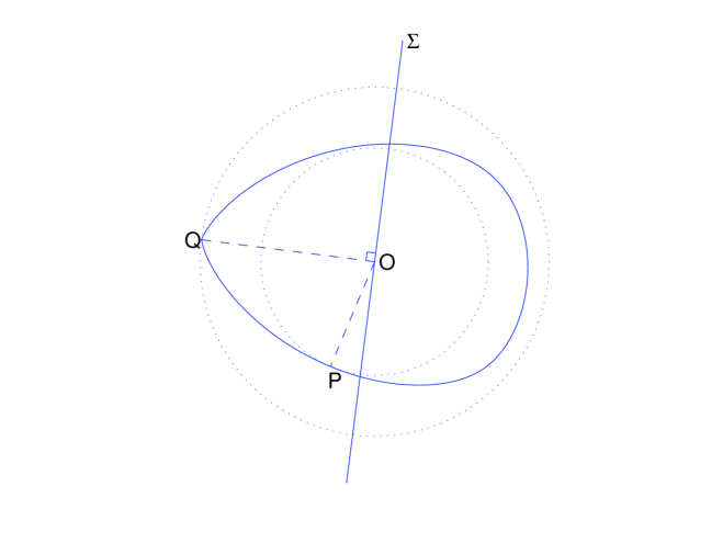
Figure 2: The farthest segment $\Sigma$ for the Hausdorff distance.

Proof.

Let $B_{1}$ be the largest ball centered at $O$ and contained in $C$ and $B_{2}$ the smallest ball centered at O which contains $C$. We denote by $R_{1}$ (resp. $R_{2}$) the radius of $B_{1}$ (resp. $B_{2}$). Let $P$, resp. $Q$, be contact points of these balls with the boundary of $C$ (see Figure 2). We also denote by $\Sigma_{1}$ the segment (centered at 0) containing $P$ and by $\Sigma$ the segment (centered at 0) orthogonal to $OQ$.

It is easy to see that $\Sigma_{1}$ is optimal, among all segments $S$, to maximize $\rho(S,C)$ while $\Sigma$ is optimal to maximize $\rho(C,S)$. Now, we are going to prove that, for any convex set $K$ in ${\mathcal{A}}$:

$$\rho(K,C)\leq\rho(\Sigma_{1},C)\quad\mbox{and}\quad\rho(C,K)\leq\rho(C,\Sigma)\,.$$ (29)

For the first inequality, let us consider any point $M$ in $K$. By construction of the ball $B_{1}$:

$$d(M,C)\leq d(M,B_{1})=OM-R_{1}\,.$$

Now, by the first inequality of theorem 3.1, $OM\leq Per(K)/4=\pi/2$ and the result follows taking the supremum in $M$ since $\rho(\Sigma_{1},C)=\pi/2-R_{1}$.

We prove now the second inequality in (29) for any convex body $K$ (the result is already clear for segments as mentioned above). Since the Steiner point lies in the interior, for any point $M\in\partial C$

$$d(M,K)<OM\leq OQ=\rho(C,\Sigma)\,.$$

Therefore, taking the supremum in $M$, $\rho(C,K)\leq\rho(C,\Sigma)$.
From (29) it follows that for any set $K$:

$$d_{H}(K,C)\leq\max(d_{H}(\Sigma_{1},C),d_{H}(\Sigma,C))\,.$$

Now, we use the second inequality in Theorem 3.1, which can be written

$$\rho(\Sigma_{1},C)=\pi/2-R_{1}\leq R_{2}=\rho(C,\Sigma)\,.$$

Since, however, $\rho(C,\Sigma_{1})\leq\rho(C,\Sigma)$, we have

$$d_{H}(\Sigma_{1},C)\leq\rho(C,\Sigma)\leq d_{H}(\Sigma,C)$$

which gives the desired result. ∎

3.3 The farthest convex set for the $L^{2}$ distance

For the $L^{2}$ distance, the result is similar: the convex set farthest from any given convex set will be a segment. The proof is more complicated and relies on our Theorem 2.3.

Theorem 3.5.

If $C$ is a given convex set in the class ${\mathcal{A}}$, then the convex set $K_{C}$ for which

$$d_{2}(C,K_{C})=\max\{d_{2}(C,K):K\in{\mathcal{A}}\}$$

is a segment. More precisely, it is any segment $\Sigma_{\alpha}$ with $\alpha$ which maximizes the one variable function $\alpha\mapsto\int_{0}^{\pi}h_{C}(\theta+\alpha)\sin\theta\,d\theta$.

Proof.

In the proof we denote by $C$ a fixed convex set in the class ${\mathcal{A}}$. An immediate consequence of Theorem 2.3 applied to the functional $J$ defined by

$$J(K)=\int_{0}^{2\pi}(h_{K}-h_{C})^{2}\,d\theta=\int_{0}^{2\pi}h_{K}^{2}-2h_{C}h_{K}(+h_{C}^{2})\,d\theta$$

is that the farthest convex set is either a triangle or a segment. Thus, to prove the result, we need to exclude the first possibility.

Let $T$ be a triangle that we assume to be a critical point for the functional $J:K\mapsto d_{2}^{2}(C,K)$. Each triangle in the class ${\mathcal{A}}$ will be uniquely characterized by its three angles $(\theta_{1},\theta_{2},\theta_{3})$ such that $e^{i\theta_{k}}$ is the normal vector to each side. The only restrictions we need to put on these angles are

$$0<\theta_{2}-\theta_{1}<\pi,\;0<\theta_{3}-\theta_{2}<\pi,\;0<2\pi+\theta_{1}-\theta_{3}<\pi,\,.$$ (30)

The lengths of the sides will be denoted by $a_{1},a_{2},a_{3}$. According to the law of sines, given that the perimeter of $T$ is $2\pi$, the three lengths are given by:

$$\begin{array}[]{l}a_{1}=\dfrac{2\pi sin(\theta_{3}-\theta_{2})}{sin(\theta_{3}-\theta_{2})+sin(\theta_{2}-\theta_{1})+sin(\theta_{1}-\theta_{3})},\\ a_{2}=\dfrac{2\pi sin(\theta_{1}-\theta_{3})}{sin(\theta_{3}-\theta_{2})+sin(\theta_{2}-\theta_{1})+sin(\theta_{1}-\theta_{3})},\\ a_{3}=\dfrac{2\pi sin(\theta_{2}-\theta_{1})}{sin(\theta_{3}-\theta_{2})+sin(\theta_{2}-\theta_{1})+sin(\theta_{1}-\theta_{3})}\,.\end{array}$$ (31)

Note that the denominator $sin(\theta_{3}-\theta_{2})+sin(\theta_{2}-\theta_{1})+sin(\theta_{1}-\theta_{3})$ can also be written $4sin(\frac{\theta_{3}-\theta_{2}}{2})sin(\frac{\theta_{2}-\theta_{1}}{2})sin(\frac{\theta_{1}-\theta_{3}}{2})$.

If $A_{1},A_{2},A_{3}$ denote the vertices of the triangle, from the relation $\vec{A_{1}A_{2}}+\vec{A_{2}A_{3}}+\vec{A_{3}A_{1}}=\vec{0}$ rotated by $\pi/2$, we get

$$a_{1}\cos\theta_{1}+a_{2}\cos\theta_{2}+a_{3}\cos\theta_{3}=0\quad\mbox{and}\quad a_{1}\sin\theta_{1}+a_{2}\sin\theta_{2}+a_{3}\sin\theta_{3}=0\,.$$ (32)

The support function (with the Steiner point at the origin) $h_{T}(\theta)$ of the triangle $T$ can be calculated with the aid of formula (5) using the fact that the radius of curvature of $T$ is given by $R=a_{1}\delta_{\theta_{1}}+a_{2}\delta_{\theta_{2}}+a_{3}\delta_{\theta_{3}}$, according to (1). One possible expression for $h$ is:

$$h_{T}(\theta)=\left\{\begin{array}[]{lc}\displaystyle\frac{1}{2\pi}\sum_{k=1}^{3}a_{k}\theta_{k}\sin(\theta-\theta_{k}),&\theta\leq\theta_{1}\,\mbox{or}\,\theta\geq\theta_{3}\\ \displaystyle\frac{1}{2\pi}\sum_{k=1}^{3}a_{k}\theta_{k}\sin(\theta-\theta_{k})+a_{1}\sin(\theta-\theta_{1}),&\theta_{1}\leq\theta\leq\theta_{2}\\ \displaystyle\frac{1}{2\pi}\sum_{k=1}^{3}a_{k}\theta_{k}\sin(\theta-\theta_{k})-a_{3}\sin(\theta-\theta_{3}),&\theta_{2}\leq\theta\leq\theta_{3},\end{array}\right.$$ (33)

where we have used the fact that, by (32) for any $\theta$, $\sum_{k=1}^{3}a_{k}\sin(\theta-\theta_{k})=0$. We will denote by $\phi(\theta)$ the function

$$\phi(\theta)=\frac{1}{2\pi}\sum_{k=1}^{3}a_{k}\theta_{k}\sin(\theta-\theta_{k})\,.$$

Now, if $T$ is a critical point of the functional $\int_{0}^{2\pi}(h_{K}-h_{C})^{2}\,d\theta$ among any convex set in ${\mathcal{A}}$, it is also a critical point among triangles. So we can express that the derivatives with respect to $\theta_{1},\theta_{2},\theta_{3}$ of

$$J(\theta_{1},\theta_{2},\theta_{3})=\int_{0}^{2\pi}(h_{T}-h_{C})^{2}\,d\theta\,,$$

where $h_{T}$ is defined in (33), are zero, that is

$$\int_{0}^{2\pi}(h_{T}-h_{C})\dfrac{\partial h_{T}}{\partial\theta_{j}}\,d\theta=0,\ j=1,2,3\,.$$

According to (33), we have (note that $h_{T}$ is continuous):

$$\begin{array}[]{l}\vspace{2mm}\dfrac{\partial h_{T}}{\partial\theta_{1}}=\dfrac{\partial\phi}{\partial\theta_{1}}+(\dfrac{\partial a_{1}}{\partial\theta_{1}}\sin(\theta-\theta_{1})-a_{1}\cos(\theta-\theta_{1}))\chi_{[\theta_{1},\theta_{2}]}-\dfrac{\partial a_{3}}{\partial\theta_{1}}\sin(\theta-\theta_{3})\chi_{[\theta_{2},\theta_{3}]}\,,\\ \vspace{2mm}\dfrac{\partial h_{T}}{\partial\theta_{2}}=\dfrac{\partial\phi}{\partial\theta_{2}}+\dfrac{\partial a_{1}}{\partial\theta_{2}}\sin(\theta-\theta_{1})\chi_{[\theta_{1},\theta_{2}]}-\dfrac{\partial a_{3}}{\partial\theta_{2}}\sin(\theta-\theta_{3})\chi_{[\theta_{2},\theta_{3}]}\,,\\ \dfrac{\partial h_{T}}{\partial\theta_{3}}=\dfrac{\partial\phi}{\partial\theta_{3}}+\dfrac{\partial a_{1}}{\partial\theta_{3}}\sin(\theta-\theta_{1})\chi_{[\theta_{1},\theta_{2}]}-(\dfrac{\partial a_{3}}{\partial\theta_{3}}\sin(\theta-\theta_{3})-a_{3}\cos(\theta-\theta_{3}))\chi_{[\theta_{2},\theta_{3}]}\,.\end{array}$$ (34)

But since $\frac{\partial\phi}{\partial\theta_{j}}$, for $j=1,2,3$ is a linear combination of $\sin(\theta-\theta_{k})$ and $\cos(\theta-\theta_{k})$, the contributions $\int_{0}^{2\pi}(h_{T}-h_{C})\dfrac{\partial\phi}{\partial\theta_{k}}\,d\theta$ are zero because $\int_{0}^{2\pi}h\cos\theta d\theta=\int_{0}^{2\pi}h\sin\theta d\theta=0$ for both $h_{T}$ and $h_{C}$. Therefore, the optimality conditions at the critical triangle $T$ can be written

$$\left\{\begin{array}[]{l}\dfrac{\partial a_{1}}{\partial\theta_{1}}\int_{\theta_{1}}^{\theta_{2}}(h_{T}-h_{C})\sin(\theta-\theta_{1})-a_{1}\int_{\theta_{1}}^{\theta_{2}}(h_{T}-h_{C})\cos(\theta-\theta_{1})-\\ \hskip 28.45274pt\dfrac{\partial a_{3}}{\partial\theta_{1}}\int_{\theta_{2}}^{\theta_{3}}(h_{T}-h_{C})\sin(\theta-\theta_{3})=0\\ \dfrac{\partial a_{1}}{\partial\theta_{2}}\int_{\theta_{1}}^{\theta_{2}}(h_{T}-h_{C})\sin(\theta-\theta_{1})-\dfrac{\partial a_{3}}{\partial\theta_{2}}\int_{\theta_{2}}^{\theta_{3}}(h_{T}-h_{C})\sin(\theta-\theta_{3})=0\\ \dfrac{\partial a_{1}}{\partial\theta_{3}}\int_{\theta_{1}}^{\theta_{2}}(h_{T}-h_{C})\sin(\theta-\theta_{1})+a_{3}\int_{\theta_{2}}^{\theta_{3}}(h_{T}-h_{C})\cos(\theta-\theta_{3})-\\ \hskip 28.45274pt\dfrac{\partial a_{3}}{\partial\theta_{3}}\int_{\theta_{2}}^{\theta_{3}}(h_{T}-h_{C})\sin(\theta-\theta_{3})=0\,.\\ \end{array}\right.$$ (35)

Using (31) we can explicitly compute each partial derivative $\frac{\partial a_{i}}{\partial\theta_{j}}$. For example, for $a_{1}$ they work out to be

$$\begin{array}[]{l}\vspace{2mm}\dfrac{\partial a_{1}}{\partial\theta_{2}}=\frac{\pi}{2}\cot\frac{\theta_{1}-\theta_{3}}{2}\frac{1}{\sin^{2}\frac{\theta_{2}-\theta_{1}}{2}},\quad\dfrac{\partial a_{1}}{\partial\theta_{3}}=-\frac{\pi}{2}\cot\frac{\theta_{2}-\theta_{1}}{2}\frac{1}{\sin^{2}\frac{\theta_{1}-\theta_{3}}{2}}\\ \dfrac{\partial a_{1}}{\partial\theta_{1}}=-\dfrac{\partial a_{1}}{\partial\theta_{2}}-\dfrac{\partial a_{1}}{\partial\theta_{3}}=-\frac{\pi}{4}\dfrac{\sin(\theta_{1}-\theta_{2})+\sin(\theta_{1}-\theta_{3})}{\sin^{2}\frac{\theta_{2}-\theta_{1}}{2}\sin^{2}\frac{\theta_{1}-\theta_{3}}{2}}\,.\end{array}$$ (36)

In order to simplify the partial derivatives, we introduce the following integrals:

$$\begin{array}[]{ccc}I_{1}=\int_{\theta_{1}}^{\theta_{2}}(h_{T}-h_{C})\sin(\theta-\theta_{1})&I_{2}=\int_{\theta_{1}}^{\theta_{2}}(h_{T}-h_{C})\sin(\theta-\theta_{2})\\ J_{1}=\int_{\theta_{2}}^{\theta_{3}}(h_{T}-h_{C})\sin(\theta-\theta_{2})&J_{2}=\int_{\theta_{2}}^{\theta_{3}}(h_{T}-h_{C})\sin(\theta-\theta_{3})\\ K_{1}=\int_{\theta_{3}}^{\theta_{1}+2\pi}(h_{T}-h_{C})\sin(\theta-\theta_{3})&K_{2}=\int_{\theta_{3}}^{\theta_{1}+2\pi}(h_{T}-h_{C})\sin(\theta-\theta_{1})\end{array}$$ (37)

In consequence, the second equality in (35) simplifies to:

$$\dfrac{1}{\sin^{2}\frac{\theta_{2}-\theta_{1}}{2}}\,I_{1}+\dfrac{1}{\sin^{2}\frac{\theta_{3}-\theta_{2}}{2}}\,J_{2}=0$$ (38)

We also introduce the integral

$$I=\int_{0}^{2\pi}(h_{T}-h_{C})h_{T}\,d\theta$$ (39)

which is nothing else than half the derivative of the functional $J$ at $h_{T}$. Using the notation (37) and formulae (33), together with the fact that $\int_{0}^{2\pi}(h_{T}-h_{C})\phi\,d\theta=0$, we get: $I=a_{1}I_{1}-a_{3}J_{2}$. Thanks to (31) and (38), we can express $I_{1}$ and $J_{2}$ in terms of $I$:

$$I=-\dfrac{1}{2\sin^{2}\frac{\theta_{2}-\theta_{1}}{2}}\,I_{1}=\dfrac{1}{2\sin^{2}\frac{\theta_{3}-\theta_{2}}{2}}\,J_{2}\,.$$ (40)

Obviously, by symmetry and using other equivalent expressions of the support function $h_{T}$, we can also conclude that

$$I=-\dfrac{1}{2\sin^{2}\frac{\theta_{3}-\theta_{2}}{2}}\,J_{1}=\dfrac{1}{2\sin^{2}\frac{\theta_{1}-\theta_{3}}{2}}\,K_{2}=-\dfrac{1}{2\sin^{2}\frac{\theta_{1}-\theta_{3}}{2}}\,K_{1}=\dfrac{1}{2\sin^{2}\frac{\theta_{2}-\theta_{1}}{2}}\,I_{2}\,.$$ (41)

Note that we can easily express any of the integrals $\int_{\theta_{j}}^{\theta_{j+1}}(h_{T}-h_{C})\sin\theta\,d\theta$ or $\int_{\theta_{j}}^{\theta_{j+1}}(h_{T}-h_{C})\cos\theta\,d\theta$ in terms of the six integrals defined in (37) and therefore entirely in terms of $I$.

Now summing the three equations in (35) and taking into account that $\frac{\partial a_{1}}{\partial\theta_{1}}+\frac{\partial a_{1}}{\partial\theta_{2}}+\frac{\partial a_{1}}{\partial\theta_{3}}=0$, and the analogous relation for $a_{3}$, yields

$$a_{3}\int_{\theta_{2}}^{\theta_{3}}(h_{T}-h_{C})\cos(\theta-\theta_{3})-a_{1}\int_{\theta_{1}}^{\theta_{2}}(h_{T}-h_{C})\cos(\theta-\theta_{1})=0\,.$$

We can use the previous expressions to write this last inequality in terms of the integral $I$, so that

$$\cos\left(\frac{\theta_{3}-\theta_{2}}{2}\right)(\sin(\theta_{2}-\theta_{1})-\sin(\theta_{1}-\theta_{3}))\,I=0\,.$$ (42)

By symmetry, we get the similar relations obtained by permutation. Since the cosine is positive (the difference between two angles is less than $\pi$), we deduce from relation (42) and its analogues that

1. either $I=0$

2. or $\theta_{3}-\theta_{2}=\theta_{2}-\theta_{1}=2\pi+\theta_{1}-\theta_{3}$, that is, $T$ is an equilateral triangle.

Now, in the case of an equilateral triangle, it is also possible to simplify the integral $I$. The support function $h_{T}$ of the equilateral triangle $\theta_{1},\theta_{2}=\theta_{1}+2\pi/3,\theta_{3}=\theta_{1}+4\pi/3$ is also given by:

$$h_{T}(\theta)=\left\{\begin{array}[]{lc}\dfrac{2\pi}{3\sqrt{3}}\,\cos(\theta-\theta_{1}-\pi/3)&\theta_{1}\leq\theta\leq\theta_{2}\\ \dfrac{2\pi}{3\sqrt{3}}\,\cos(\theta-\theta_{1}-\pi)&\theta_{2}\leq\theta\leq\theta_{3}\\ \dfrac{2\pi}{3\sqrt{3}}\,\cos(\theta-\theta_{1}-5\pi/3)&\theta_{3}\leq\theta\leq\theta_{1}+2\pi\,.\\ \end{array}\right.$$ (43)

Then we have:

$$\begin{array}[]{l}I=\dfrac{2\pi}{3\sqrt{3}}\left(\int_{\theta_{1}}^{\theta_{2}}(h_{T}-h_{C})\cos(\theta-\theta_{1}-\pi/3)+\int_{\theta_{2}}^{\theta_{3}}(h_{T}-h_{C})\cos(\theta-\theta_{1}-\pi)\right.\\ \qquad\ \left.+\int_{\theta_{3}}^{\theta_{1}+2\pi}(h_{T}-h_{C})\cos(\theta-\theta_{1}-5\pi/3)\right)\,.\end{array}$$

Using the notation introduced in (37), a straightforward computation produces

$$I=\dfrac{2\pi}{9}\left(I_{1}-I_{2}+J_{1}-J_{2}+K_{1}-K_{2}\right)\,.$$

Now, replacing each $I_{1},I_{2},\ldots$ on the right side by its expression in terms of $I$ obtained in (40), Eq. (41) yields $I=-2\pi I$. Thus, we also get $I=0$ in this case.

To conclude the proof, it remains to show that it is impossible that $I=0$ at a (local) maximum. Thus, let us assume that $I$, as defined in (39), is equal to 0. We consider the family of convex sets $K_{t}=(1-t)T+t\Sigma_{\alpha}$ where $\Sigma_{\alpha}$ is a segment. The derivative of $t\mapsto J(K_{t},C)$ at $t=0$ is $2\int_{0}^{2\pi}(h_{T}-h_{C})(h_{\Sigma_{\alpha}}-h_{T})\,d\theta$. Since $I=0$, this derivative is actually

$$g(\alpha):=\pi\int_{0}^{2\pi}(h_{T}-h_{C})(\theta)|\sin(\theta-\alpha)|\,d\theta\,.$$

We can also write $g(\alpha)$ as

$$g(\alpha):=\pi\int_{0}^{\pi}(h_{T}-h_{C})(\theta+\alpha)\sin(\theta)\,d\theta\,.$$

Now this function of $\alpha$ is $\pi$-periodic, continuous and its integral over $(0,2\pi)$ is

$$\pi\int_{0}^{2\pi}\int_{0}^{\pi}(h_{T}-h_{C})(\theta+\alpha)\sin(\theta)\,d\theta d\alpha=0\,.$$

Therefore, either $g(\alpha)$ takes positive and negative values, in which case $T$ cannot be a local maximizer, or else $g(\alpha)$ is identically 0. In the latter case, we come back to the optimality condition (among all convex sets) given in Theorem 2.2. There exist $\xi_{0}\in H^{1}(\mathbb{T})$, nonpositive, vanishing on the support of $T$, and $\mu\in\mathbb{R}$ such that, for any $v\in H^{1}(\mathbb{T})$, the derivative of the functional is given by

$$<dJ(T),v>=\int_{0}^{2\pi}(h_{T}-h_{C})v(\theta)\,d\theta=<\xi_{0}+{\xi_{0}}^{\prime\prime},v>+\mu\int_{0}^{2\pi}v\,d\theta\,.$$ (44)

Applying (44) to $v=h_{\Sigma_{\alpha}}-h_{T}$, since the left side is zero and $\int_{0}^{2\pi}h_{\Sigma_{\alpha}}=\int_{0}^{2\pi}h_{T}=2\pi$, it follows that for any $\alpha\in(0,\pi)$, $\xi_{0}(\alpha)+\xi_{0}(\alpha+\pi)=0$. Since $\xi_{0}\leq 0$, this implies that $\xi_{0}=0$. Now applying (44) once again to $v=h_{\Sigma_{\alpha}}$, we get

$$0=\int_{0}^{2\pi}(h_{T}-h_{C})h_{\Sigma_{\alpha}}\,d\theta=2\pi\mu.$$

Thus $\mu=0$ and the derivative of the $L^{2}$ distance at $T$ is identically zero. This implies that $C=T$, and is thus actually the global minimizer.

The final claim of the theorem follows easily from the expansion

$$\int_{0}^{2\pi}(h_{\Sigma_{\alpha}}-h_{C})^{2}\,d\theta=\frac{\pi^{3}}{4}+\int_{0}^{2\pi}h_{C}^{2}\,d\theta-\pi\int_{0}^{2\pi}h_{C}|\sin(\theta-\alpha)|\,d\theta$$

and the equality

$$\int_{0}^{2\pi}h_{C}|\sin(\theta-\alpha)|\,d\theta=2\int_{0}^{\pi}h_{C}(\theta+\alpha)\sin\theta\,d\theta\,.$$

∎

Remark 3.

The farthest segment according to the $L^{2}$ distance is not necessarily unique. Apart from the trivial example of a disc, for a body of constant width, every segment in ${\mathcal{A}}$ is equally distant. This can easily be seen using the Fourier series expansion of the support function of a body of constant width $C$, which is known to contain only odd terms other than the constant:

$$h_{C}(\theta)=1+\sum_{k=-\infty,\,k\not=-1,1}^{+\infty}c_{2k+1}e^{(2k+1)i\theta},$$

while the Fourier series expansion of the support function $h_{\alpha}$ of a segment $\Sigma_{\alpha}$ contains only even terms. This is due to the relation ${h^{\prime\prime}}_{\alpha}+h_{\alpha}=\frac{\pi}{2}(\delta_{\alpha}+\delta_{\pi+\alpha})$, which when applied to $e^{-in\theta}$ yields the following equality for the $n$-th Fourier coefficient $\gamma_{n}$ of $h_{\alpha}$:

$$(1-n^{2})\gamma_{n}=\frac{\pi}{2}\,e^{-in\alpha}(1+e^{-in\pi})\,.$$

The $L^{2}$ distance between $C$ and $\Sigma_{\alpha}$ is

$$d_{2}(C,\Sigma_{\alpha})=\int_{0}^{2\pi}h_{\alpha}^{2}\,d\theta-2\int_{0}^{2\pi}h_{C}h_{\alpha}\,d\theta+\int_{0}^{2\pi}h_{C}^{2}\,d\theta\,.$$

Now, using the Parseval relation and the orthogonality properties of the Fourier coefficients of the two support functions, we see that the integral $\int_{0}^{2\pi}h_{C}h_{\alpha}\,d\theta$ is always equal to $2\pi$, and therefore the $L^{2}$ distance between $C$ and a segment does not depend on the segment within the class ${\mathcal{A}}$.

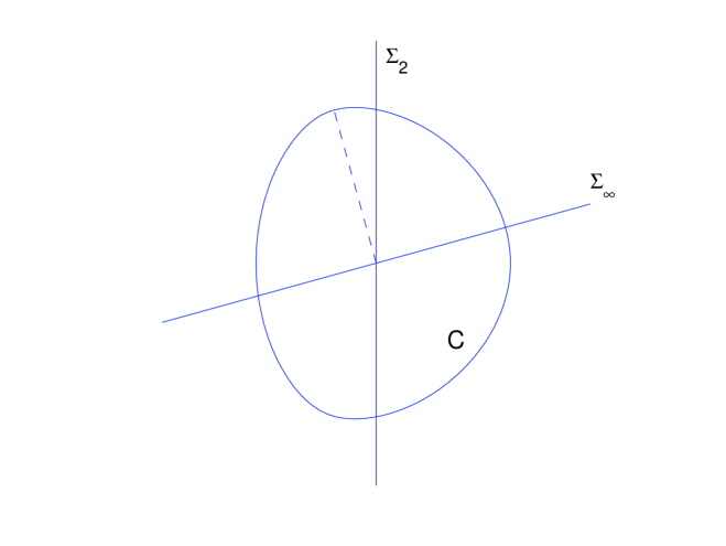
Figure 3: The farthest segments $\Sigma_{2}$ and $\Sigma_{\infty}$ do not generally coincide.

Remark 4.

The farthest segment for the $L^{2}$ distance and for the Hausdorff distance do not generally coincide. The Figure 3 shows the farthest segment $\Sigma_{2}$ (for the $L^{2}$ distance) and $\Sigma_{\infty}$ (for the Hausdorff distance) of the convex set $C$ whose support function is $h_{C}(\theta)=1-0.1\cos(2\theta)+0.05\cos(3\theta)$.

References

- [1] P. Exner, M. Fraas, E. M. Harrell II, On the critical exponent in an isoperimetric inequality for chords, Physics Letters, A 368 (2007), 1-6.
- [2] P. Exner, E. M. Harrell II, M. Loss, Inequalities for means of chords, with application to isoperimetric problems, Letters in Math. Phys., 75 (2006), 225-233. Addendum, Ibid., 77(2006)219.
- [3] H. Groemer, Geometric applications of Fourier series and spherical harmonics, Encycl. Math. and Appl. 61, Cambridge: Cambridge Univ. Press, 1996.
- [4] P.M. Gruber, The space of convex bodies, Handbook of convex geometry, P.M. Gruber and J.M. Wills eds, Elsevier 1993, pp. 301-318.
- [5] E. M. Harrell II, A. Henrot, On the maximum of a class of functionals on convex regions, and the means of chords weighted by curvature, in prep.
- [6] A. Henrot, M. Pierre, Variation et optimisation de formes, Mathématiques et Applications 48, Springer, 2005.
- [7] T. Lachand-Robert, M.A. Peletier, Newton’s problem of the body of minimal resistance in the class of convex developable functions, Math. Nachr., 226 (2001), 153–176.
- [8] J. Lamboley, A. Novruzi, Polygons as optimal shapes with convexity constraint, to appear.
- [9] D.E. McClure, R.A. Vitale, Polygonal approximation of plane convex bodies,J. Math. Anal. Appl. 51 (1975), 326-358.
- [10] P. McMullen, The Hausdorff distance between compact convex sets, Mathematika, 31 (1984), 76-82.
- [11] H. Maurer, J. Zowe, First and second order necessary and sufficient optimality conditions for infinite-dimensional programming problems, Math. Programming, 16 (1979), no. 1, 98-110.
- [12] G. Pólya, G. Szegő, Isoperimetric inequalities in mathematical physics, Annals of Mathematics Studies AM-27. Princeton: Princeton University Press, 1951.
- [13] R. T. Rockafellar, Convex Analysis, Princeton University Press, 1970.
- [14] R. Schneider, Convex bodies: the Brunn-Minkowski Theory, Encyclopedia of Mathematics and its Applications, Cambridge University Press 1993.
- [15] R. Webster, Convexity, Oxford University Press, 1994.