Chapter 0 Notes on the Statistical Mechanics of Systems with Long-Range Interactions

David Mukamel

Department of Physics, The Weizmann Institute of Science,

Rehovot, 76100, Israel

URL: http://www.weizmann.ac.il/home/fnmukaml/

1 Introduction

In these Notes we discuss some thermodynamic and dynamical properties of models of systems in which the two-body interaction potential between particles decays algebraically with their relative distance $r$ at large distances. Typically the potential decays as $1/r^{d+\sigma}$ in $d$ dimensions and it may either be isotropic or non-isotropic (as in the case of magnetic or electric dipolar interactions). In general one can distinguish between two broad classes long range interactions (LRI). Those with $-d\leq\sigma\leq 0$ which we term ”strong” LRI, and those with $0<\sigma\leq\sigma_{c}(d)$ which we term ”weak” LRI. The parameter $\sigma_{c}(d)$ satisfies $\sigma_{c}(d)=2$ for $d\geq 4$, and $\sigma_{c}(d)=d/2$ for $d<4$, as will be discussed in more detail in the following sections. In systems with strong LRI the potential decays slowly with the distance, and it results in rather pronounced thermodynamic and dynamical effects . On the other hand in systems with weak LRI the potential decays faster at large distances, resulting in less pronounced effects. Systems with $\sigma>\sigma_{c}$ behave thermodynamically as the more commonly studied systems with short range interactions. For recent reviews on systems with long range interactions see, for example, [(29), (20)].

Long range interactions are rather common in nature. Examples include self gravitating systems $(\sigma=-2)$ [Padmanabhan (1990), Chavanis (2002)], dipolar ferroelectrics and ferromagnets in which the interactions are anisotropic with $(\sigma=0)$ [Landau and Lifshitz (1960)], non-neutral plasmas $(\sigma=-2)$ [Nicholson (1992)], two dimensional geophysical vortices which interact via a weak, logarithmically decaying, potential $(\sigma=-2)$ [Chavanis (2002)], charged particles interacting via their mutual electromagnetic fields, such as in free electron laser [(10)] and many others.

Let us first consider strong LRI. Such systems are non-additive, and the energy of homogeneously distributed particles in a volume $V$ scales super-linearly with the volume, as $V^{1-\sigma/d}$. The lack of additivity leads to many unusual properties, both thermal and dynamical, which are not present in systems with weak LRI or with short range interactions. For example, as has first been pointed out by Antonov [Antonov (1962)] and later elaborated by Lynden-Bell [Lynden-Bell and Wood (1968), Lynden-Bell (1999)], Thirring and co-workers [Thirring (1970), Hertel and Thirring (1971), Posch and Thirring (2006)], and others, the entropy $S$ needs not be a concave function of the energy $E$, yielding negative specific heat within the microcanonical ensemble. Since specific heat is always positive when calculated within the canonical ensemble, this indicates that the two ensembles need not be equivalent. Recent studies have suggested the inequivalence of ensembles is particularly manifested whenever a model exhibits a first order transition within the canonical ensemble [(8), Barré et al (2002)]. Similar ensemble inequivalence between canonical and grand canonical ensembles has also been discussed [Misawa et al (2006)].

Typically, the entropy, $S$, which is measured by the number of ways $N$ particles with total energy $E$ may be distributed in a volume $V$, scales linearly with the volume. This is irrespective of whether or not the interactions in the system are long ranged. On the other hand, in systems with strong long range interactions, the energy scales super-linearly with the volume. Thus, in the thermodynamic limit, the free energy $F=E-TS$ is dominated by the energy at any finite temperature $T$, suggesting that the entropy may be neglected altogether. This would result in trivial thermodynamics. However, in many real cases, when systems of finite size are considered, the temperature could be sufficiently high so that the entropic term in the free energy, $TS$, becomes comparable to the energy $E$. In such cases the entropy may not be neglected and the thermodynamics is non trivial. This is the case in some self gravitating systems such as globular clusters (see, for example [Chavanis (2002)]). In order to theoretically study this limit, it is convenient to rescale the energy by a factor $V^{\sigma/d}$ (or alternatively, to rescale the temperature by a factor $V^{-\sigma/d}$), making the energy and the entropy contribution to the free energy of comparable magnitude. This is known as the Kac prescription [Kac et al (1963)]. While systems described by this rescaled energy are extensive, they are non-additive in the sense that the energy of two isolated sub-systems is not equal to their total energy when they are combined together and are allowed to interact.

A special case is that of dipolar ferromagnets, where the interaction scales as $1/r^{3}$ ($\sigma=0$). In this borderline case of strong long range range interactions, the energy depends on the shape of the sample. It is well known that for ellipsoidal magnets, the contribution of the long distance part of the dipolar interaction leads to a mean-field type term in the energy. This results in an effective Hamiltonian $H\to H-DM^{2}/N$, where $M$ is the magnetization of the system and $D$ is a shape dependent coefficient known as the demagnetization factor. In this Hamiltonian, the long range interaction between dipoles becomes independent of their distance, making it particularly convenient for theoretical studies [Campa et al (2007b)].

Studies of the relaxation processes in systems with strong long range interactions in some models have shown that the relaxation of thermodynamically unstable states to the stable equilibrium state may be unusually slow, with a characteristic time which diverges with the number of particles, $N$, in the system [Antoni and Ruffo (1995), Latora et al (1998), Latora et al (1999), Yamaguchi (2003), Yamaguchi et al (2004), Mukamel et al (2005)]. This, too, is in contrast with relaxation processes in systems with short range interactions, in which the relaxation time does not scale with $N$. As a result, long lived quasi-stationary states (QSS) have been observed in some models, which in the thermodynamic limit, do not relax to the equilibrium state.

Non-additivity has been found to result, in many cases, in breaking of ergodicity. Here phase space is divided into disjoint domains separated by finite gaps in macroscopic quantities, such as the total magnetization in magnetic systems [Mukamel et al (2005), Fel’dman (1998), Borgonovi et al (2004), Borgonovi et al (2006), Hahn and Kastner (2005), Hahn and Kastner (2006), Bouchet et al (2008)]. Within local dynamics, these systems are thus trapped in one of the domains.

Features which are characteristic of non-additivity are not limited to systems with long range interactions. In fact finite systems with short range interactions, in which surface and bulk energies are comparable, are also non-additive. Features such as negative specific heat in small systems (e.g. clusters of atoms) have been discussed a number of studies [Lynden-Bell (1995), Lynden-Bell (1996), Gross (2000), Chomaz and Gulminelli (2002)].

Let us turn now to systems with weak long range interaction, for which $0<\sigma\leq\sigma_{c}(d)$. These systems are additive, namely, the energy of a homogeneously distributed particles scales as $V$. As a result, the usual formulation of thermodynamics and statistical mechanics developed for systems with short range interactions directly apply in this case. In particular the specific heat is non-negative as expected, and the various statistical mechanical ensembles are equivalent. However, the long range nature of the interaction becomes dominant at phase transitions, where long range correlations are naturally built up in the system. For example it is well known that one dimensional ($1d$) systems with short range interactions do not exhibit phase transitions and spontaneous symmetry breaking at finite temperatures. On the other hand weak long range interactions may result in phase transitions in one dimension at a finite temperature. A notable example of such a transition has been introduced by Dyson in the sixties [Dyson ( 1969a), Dyson ( 1969b)].

The critical behavior of systems near a continuous phase transition is commonly classified by universality classes. The critical exponents of each class do not depend on the details of the interactions but rather on some general features such as the spatial dimension of the system, its symmetry and range of forces. Weak long range interactions modify the universality class of the system leading to critical exponents which depend on the interaction parameter $\sigma$. It is also well known that the critical behavior of systems with short range interactions become mean-field like above a critical dimension $d_{c}$, where the effect of fluctuations may be neglected. For a generic critical point in a system with short range interactions one has $d_{c}=4$. Since long range interactions tend to reduce fluctuations, weak LRI result in a smaller critical dimension, $d_{c}(\sigma)$, which is a function of the interaction parameter $\sigma$, see[Fisher et al (1972), Fisher ( 1974)].

A distinct class of local interactions which are effectively weak long range in nature, when applied to long polymers, is that of excluded volume interactions. This repulsive interaction, which is local in space, but which can take place between monomers which are far away along the polymer chain, can change the critical properties of the polymer, resulting in a distinct universality class. For example, while the average end-to-end distance of a polymer of length $L$ scales as $\sqrt{L}$ in a random polymer, it scales with a different power law, $L^{\nu}$, when a repulsive interaction between monomers is introduced. In general the exponent $\nu(d)$ depends on the spatial dimension of the system and it becomes equal to the value corresponding to random polymer,$1/2$, only at $d>4$. Excluded volume interactions have a profound effect on the thermodynamic behavior of polymer solutions, DNA denaturation and many other systems of long polymers, see, for example, [Des Cloizeax and Jannink (1990)]. We will not discuss excluded volume effects in these Notes.

We now turn to systems out of thermal equilibrium. In many cases driven systems reach a non-equilibrium steady state in which detailed balance is not satisfied. Under rather broad conditions such steady states in systems with conserving dynamics exhibit long range correlations, even when the dynamics is local. In thermal equilibrium, the nature of the equilibrium state is independent of the dynamics involved. For example an Ising model evolving under magnetization conserving Kawasaki dynamics, reaches the same equilibrium state as that reached by a non-conserving Glauber dynamics. The equilibrium state is uniquely determined by the Hamiltonian. This is not the case in non-equilibrium systems, and the resulting steady state is strongly affected by the details of the dynamics. Conserved quantities tend to introduce long range correlations in the steady state, due to the slow diffusive nature of their dynamics. At equilibrium these long range correlations are somehow canceled due to detailed balance which lead to the Gibbs equilibrium distribution. Under non-equilibrium conditions, such cancelation does not take place generically. Therefore, one expects properties of of equilibrium systems with long range interactions to show up in steady states of non-equilibrium systems with conserving local interactions.

Long range correlations have been studies a large number of driven models. For example, as discussed above, one dimensional equilibrium systems with short range interactions do not exhibit phase transitions or spontaneous symmetry breaking at finite temperatures. In equilibrium, phase transitions in $1d$ systems take place only when long range interactions are present. On the other hand quite a number of models of driven one dimensional systems have been shown to display phase transitions and spontaneous symmetry breaking even when their dynamics is local, see [Mukamel (2000)]. This demonstrates the build-up of long range correlations by the driving dynamical processes. An interesting model in this respect is what is known as the $ABC$ model. This is a model of three species of particles, $A$, $B$ and $C$, which move on a ring with local dynamical rules, reaching a steady state in which the three species are spatially separated. The dynamical rules do not obey detailed balance, and hence the model is out of equilibrium. It has been demonstrated that the dynamics of this model result in effective long range interactions, which can be explicitly calculated [Evans et al (1998a), Evans et al (1998b)]. The model will be discussed in some detail in these Notes.

The Notes are organized as follows: in Section 2 we discuss properties of systems with strong long range interactions. Some properties of weak long range interactions, particularly, the existence of long range order in $1d$ and the upper critical dimension are discussed in Section 3. Effective long range interactions in drive models, are demonstrated within the context of the $ABC$ model in Section 4. Finally, a brief summary is given in Section 5.

2 Strong Long Range Interactions

1 General Considerations

We start by presenting some general considerations concerning thermodynamic properties of systems with strong long range interactions. In particular we argue that in addition to negative specific heat, or non-concave entropy curve, which could be realized in the microcanonical ensemble, this ensemble also yields discontinuity in temperature whenever a first order transition takes place.

Consider the non-concave curve of Fig. (1). For a system with short range interactions, this curve cannot represent the entropy $S(E)$. The reason is that due to additivity, the system represented by this curve is unstable in the energy interval $E_{1}<E<E_{2}$. Entropy can be gained by phase separating the system into two subsystems corresponding to $E_{1}$ and $E_{2}$ keeping the total energy fixed. The average energy and entropy densities in the coexistence region is given by the weighted average of the corresponding densities of the two coexisting systems. Thus the correct entropy curve in this region is given by the common tangent line, resulting in an overall concave curve. However, in systems with strong long range interactions, the average energy density of two coexisting subsystems is not given by the weighted average of the energy density of the two subsystems. Therefore, the non-concave curve of Fig. (1) could, in principle, represent an entropy curve of a stable system, and phase separation need not take place. This results in negative specific heat. Since within the canonical ensemble specific heat is non-negative, the microcanonical and canonical ensembles are not equivalent. The above considerations suggest that the inequivalence of the two ensembles is particularly manifested whenever a coexistence of two phases is found within the canonical ensemble.

Another feature of systems with strong long range interactions is that within the microcanonical ensemble, first order phase transitions involve discontinuity of temperature. To demonstrate this point consider, for example, a magnetic system which undergoes a phase transition from a paramagnetic to a magnetically ordered phase. Let $M$ be the magnetization and $S(M,E)$ be the entropy of the system for a given magnetization and energy. A typical entropy vs magnetization curve for a given energy close to a first order transition is given in Fig. (2). It exhibits three local maxima, one at $M=0$ and two other degenerate maxima at $\pm M_{0}$. At energies where the paramagnetic phase is stable, one has $S(0,E)>S(\pm M_{0},E)$. In this phase the entropy is given by $S(0,E)$ and the temperature is obtained by $1/T=dS(0,E)/dE$. On the other hand at energies where the magnetically ordered phase is stable, the entropy is given by $S(M_{0},E)$ and the temperature is $1/T=dS(M_{0},E)/dE$. At the first order transition point, where $S(0,E)=S(\pm M_{0},E)$, the two derivatives are generically not equal, resulting in a temperature discontinuity. A typical entropy vs energy curve is given in Fig. (3). Note that these considerations do not apply to systems with short range interactions. The reason is that the entropy of these systems is a concave function of the two extensive parameters $M$ and $E$, and the transition involves discontinuities of both parameters..

Systems with long range interactions are more likely to exhibit breaking of ergodicity due to their non-additive nature. This may be argued on rather general grounds. In systems with short range interactions, the domain in the phase space of extensive thermodynamic variables, such as energy, magnetization, volume etc., is convex. Let $\vec{X}$ be a vector whose components are the extensive thermodynamic variables over which the systems is defined. Suppose that there exist microscopic configurations corresponding to two points $\vec{X}_{1}$ and $\vec{X}_{2}$ in this phase space. As a result of the additivity property of systems with short range interactions, there exist microscopic configurations corresponding to any intermediate point between $\vec{X}_{1}$ and $\vec{X}_{2}$. Such microscopic configurations may be constructed by combining two appropriately weighted subsystems corresponding to $\vec{X}_{1}$ and $\vec{X}_{2}$, making use of the fact that for sufficiently large systems, surface terms do not contribute to bulk properties. Since systems with long range interactions are non-additive, such interpolation is not possible, and intermediate values of the extensive variables are not necessarily accessible. As a result the domain in the space of extensive variables over which a system is defined needs not be convex. When there exists a gap in phase space between two points corresponding to the same energy, local energy conserving dynamics cannot take the system from one point to the other and ergodicity is broken.

These and other features of canonical and microcanonical phase diagrams are explored in the following sections by considering specific models.

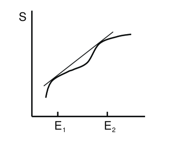
Figure 1: A non-concave entropy curve, which for additive systems is made concave by the common tangent line. In systems with long range interactions, the non-concave curve may represent the actual entropy of the system, yielding negative specific heat.

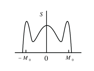
Figure 2: A typical entropy vs magnetization curve of a magnetic system with long range interactions near a first order transition at a given energy. As the energy varies the heights of the peaks change and a first order transition is obtained at the energy where the peaks are of equal height.

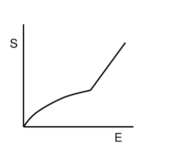
Figure 3: A typical entropy vs energy curve for a system with long range interactions exhibiting a first order transition. The slope discontinuity at the transition results in a temperature discontinuity.

2 Phase diagrams of models with strong long range interactions

In order to obtain better insight into the thermodynamic behavior of systems with strong long range interactions it is instructive to analyze phase diagrams of representative models. A particularly convenient class of models is that where the long range part of the interaction is of mean-field type. In such models $\sigma=0$, and as pointed out above, they have been applied in studies of dipolar ferromagnets [Campa et al (2007b)]. The insight obtained from studies of these models may, however, be relevant for other systems with $\sigma<0$, since the main feature of these models, namely non-additivity, is shared by models with $\sigma\leq 0$.

In recent studies both the canonical and microcanonical phase diagrams of some spin models with mean-field type long range interactions have been analyzed. Examples include discrete spin models such as the Blume-Emery-Griffiths model [(8), Barré et al (2002)] and the Ising model with long and short range interactions [Mukamel et al (2005)] as well as continuous spin models of $XY$ type [de Buyl et al (2005), Campa et al (2006)]. These models are simple enough so that their thermodynamic properties can be evaluated in both ensembles. The common feature of these models is that their phase diagrams exhibit first and second order transition lines. In has been found that in all cases, the canonical and microcanonical phase diagrams differ from each other in the vicinity of the first order transition line. A classification of possible types of inequivalent canonical and microcanonical phase diagrams in systems with long range interactions is given in [Bouchet and Barré (2005)]. In what follows we discuss in some detail the thermodynamics of one model, namely, the Ising model with long and short range interactions [Mukamel et al (2005)].

Consider an Ising model defined on a ring with $N$ sites. Let $S_{i}=\pm 1$ be the spin variable at site $i=1,\dots,N$. The Hamiltonian of the systems is composed of two interaction terms and is given by

$${}H=-\frac{K}{2}{\sum_{i=1}^{N}}\left(S_{i}S_{i+1}-1\right)-\frac{J}{2N}\left({\sum_{i=1}^{N}}S_{i}\right)^{2}.$$ (1)

The first term is a nearest neighbor coupling which could be either ferromagnetic $(K>0)$ or antiferromagnetic $(K<0)$. On the other hand the second term is ferromagnetic, $J>0$, and it corresponds to long range, mean-field type interaction. The reason for considering a ring geometry for the nearest neighbor coupling is that this is more convenient for carrying out the microcanonical analysis. Similar features are expected to take place in higher dimensions as well.

The canonical phase diagram of this model has been analyzed some time ago [Nagle (1970), Bonner and Nagle (1971), Kardar (1983)]. The ground state of the model is ferromagnetic for $K>-J/2$ and is antiferromagnetic for $K<-J/2$. Since the system is one dimensional, and since the long range interaction term can only support ferromagnetic order, it is clear that for $K<-J/2$ the system is disordered at any finite temperature, and no phase transition takes place. However, for $K>-J/2$ one expects ferromagnetic order at low temperatures. Thus a phase transition takes place at some temperature to a paramagnetic, disordered phase (see Fig. 4). For large $K$ the transition was found to be continuous, taking place at temperature given by

$$\beta=e^{-\beta K}.$$ (2)

Here $\beta=1/T$, $J=1$ is assumed for simplicity, and $k_{B}=1$ is taken for the Boltzmann constant. The transition becomes first order for $K<K_{CTP}$, with a tricritical point located at an antiferromagnetic coupling $K_{CTP}=-\ln 3/{2\sqrt{3}}\simeq-0.317$. As usual, the first order line has to be evaluated numerically. The first order line intersects the $T=0$ axis at $K=-1/2$. The $(K,T)$ phase diagram is given in Fig. (4).

Let us now analyze the phase diagram of the model within the microcanonical ensemble [Mukamel et al (2005)]. To do this one has to calculate the entropy of the system for given magnetization and energy. Let

$$U=-\frac{1}{2}\sum_{i}\left(S_{i}S_{i+1}-1\right)$$ (3)

be the number of antiferromagnetic bonds in a given configuration characterized by $N_{+}$ up spins and $N_{-}$ down spins with $N_{+}+N_{-}=N$. One would like to evaluate the number of microscopic configurations corresponding to $(N_{+},N_{-},U)$. Such configurations are composed of $U/2$ segments of up spins which alternate with the same number of segments of down spins, where the total number of up (down) spins is $N_{+}$ $(N_{-})$. The number of ways of dividing $N_{+}$ spins into $U/2$ groups is

$$\left(\begin{array}[]{c}N_{+}-1\\ U/2-1\end{array}\right)~{},\\$$ (4)

with a similar expression for the down spins. To leading order in $N$, the number of configurations corresponding to $(N_{+},N_{-},U)$ is given by

$$\Omega(N_{+},N_{-},U)=\left(\begin{array}[]{c}N_{+}\\ U/2\end{array}\right)\left(\begin{array}[]{c}N_{-}\\ U/2\end{array}\right)~{}.\\$$ (5)

Note that a multiplicative factor of order $N$ has been neglected in this expression, since only exponential terms in $N$ contribute to the entropy. This factor corresponds to the number of ways of placing the $U$ ordered segments on the lattice. Expressing $N_{+}$ and $N_{-}$ in terms of the number of spins, $N$, and the magnetization, $M=N_{+}-N_{-}$, and denoting $m=M/N$, $u=U/N$ and the energy per spin $\epsilon=E/N$, one finds that the entropy per spin, $s(\epsilon,m)=\frac{1}{N}\ln\Omega$, is given in the thermodynamic limit by

$${}s(\epsilon,m) = \frac{1}{2}(1+m)\ln(1+m)+\frac{1}{2}(1-m)\ln(1-m)$$ (6)

$$- u\ln u-\frac{1}{2}(1+m-u)\ln(1+m-u)$$

$$- \frac{1}{2}(1-m-u)\ln(1-m-u)~{},$$

where $u$ satisfies

$$\epsilon=-\frac{J}{2}m^{2}+Ku~{}\,.$$ (7)

By maximizing $s(\epsilon,m)$ with respect to $m$ one obtains both the spontaneous magnetization $m_{s}(\epsilon)$ and the entropy $s(\epsilon)\equiv s(\epsilon,m_{s}(\epsilon))$ of the system for a given energy $\epsilon$.

In order to analyze the microcanonical phase transitions corresponding to this entropy we expand $s$ in powers of $m$,

$$s=s_{0}+Am^{2}+Bm^{4}~{}.$$ (8)

Here the zero magnetization entropy is

$${}s_{0}=-\frac{\epsilon}{K}\ln\frac{\epsilon}{K}-\left(1-\frac{\epsilon}{K}\right)\ln\left(1-\frac{\epsilon}{K}\right)~{},$$ (9)

the coefficient $A$ is given by

$${}A=\frac{1}{2}\left[\frac{1}{K}\ln\left(\frac{K-\epsilon}{\epsilon}\right)-\frac{\epsilon}{K-\epsilon}\right]~{},$$ (10)

and $B$ is another energy dependent coefficient which can be easily evaluated. In the paramagnetic phase both $A$ and $B$ are negative so that the $m=0$ state maximizes the entropy. At the energy where $A$ vanishes, a continuous transition to the magnetically ordered state takes place. Using the thermodynamic relation for the temperature

$$\frac{1}{T}=\frac{ds}{d\epsilon}~{},$$ (11)

the caloric curve in the paramagnetic phase is found to be

$${}\frac{1}{T}=\frac{1}{K}\ln\frac{K-\epsilon}{\epsilon}~{}.$$ (12)

This expression is also valid at the critical line where $m=0$. Therefore, the critical line in the $(K,T)$ plane may be evaluated by taking $A=0$ and using (12) to express $\epsilon$ in terms of $T$. One finds that the expression for the critical line is the same as that obtained within the canonical ensemble, (2).

The transition is continuous as long as $B$ is negative, where the $m=0$ state maximizes the entropy. The transition changes its character at a microcanonical trictitical point where $B=0$. This takes place at $K_{MTP}\simeq-0.359$, which may be computed analytically using the expression for the coefficient $B$. The fact that $K_{MTP}<K_{CTP}$ means that while the microcanonical and canonical critical lines coincide up to $K_{CTP}$, the microcanonical line extends beyond this point into the region where, within the canonical ensemble, the model is magnetically ordered (see Fig. (4)). In this region the microcanonical specific heat is negative. For $K<K_{MTP}$ the microcanonical transition becomes first order, and the transition line has to be evaluated numerically by maximizing the entropy. As discussed in the previous subsection, such a transition is characterized by temperature discontinuity. The shaded region in the $(K,T)$ phase diagram of Fig. (4) indicates an inaccessible domain resulting from the temperature discontinuity.

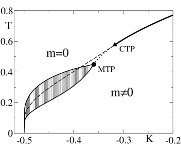
Figure 4: The $(K,T)$ phase diagrams of the model (1) within the canonical and microcanonical ensembles. In the canonical ensemble the large $K$ transition is continuous (bold solid line) down to the trictitical point CTP where it becomes first order (dashed line). In the microcanonical ensemble the continuous transition coincides with the canonical one at large $K$ (bold line). It persists at lower K (dotted line) down to the tricritical point MTP where it turns first order, with a branching of the transition line (solid lines). The region between these two lines (shaded area) is not accessible.

The main features of the phase diagram given in Fig. (4) are not peculiar to the Ising model defined by the Hamiltonian (1), but are expected to be valid for any system in which a continuous line changes its character and becomes first order at a tricritical point. In particular, the lines of continuous transition are expected to be the same in both ensembles up to the canonical tricritical point. The microcanonical critical line extends beyond this point into the ordered region of the canonical phase diagram, yielding negative specific heat. When the microcanonical tricritical point is reached, the transition becomes first order, characterized by a discontinuity of the temperature. These features have been found in studies of other discrete spin models such as the spin-$1$ Blume-Emery-Griffiths model [(8), Barré et al (2002)]. They have also been found in continuous spin models such as the $XY$ model with two- and four-spin mean-field like ferromagnetic interaction terms [de Buyl et al (2005)], and in an $XY$ model with long and short range, mean-field type, interactions [Campa et al (2006)].

3 Ergodicity breaking

Ergodicity breaking in models with long range interactions has recently been explicitly demonstrated in a number of models such as a class of anisotropic $XY$ models [Borgonovi et al (2004), Borgonovi et al (2006)], discrete spin Ising models [Mukamel et al (2005)], mean-field $\phi^{4}$ models [Hahn and Kastner (2005), Hahn and Kastner (2006)] and isotropic $XY$ models with four-spin interactions [Bouchet et al (2008)]. Here we outline a demonstration of this feature for the Ising model with long and short range interactions defined in the previous section [Mukamel et al (2005)].

Let us consider the Hamiltonian (1), and take, for simplicity, a configuration of the spins with $N_{+}>N_{-}$. The local energy $U$ is, by definition, non-negative. It also has an upper bound which, for the case $N_{+}>N_{-}$, is $U\leq 2N_{-}$. This upper bound is achieved when the negative spins are isolated, each contributing two negative bonds to the energy. Thus $0\leq u\leq 1-m$. Combining this with (7) one finds that for positive $m$ the accessible states have to satisfy

$$m\leq\sqrt{-2\epsilon}\quad,\quad m\geq m_{+}\quad,\quad m\leq m_{-}$$ (13)

$$\mbox{with}\,\,m_{\pm}=-K\pm\sqrt{K^{2}-2(\epsilon-K)}~{}.$$

Similar restrictions exist for negative $m$. These restrictions yield the accessible magnetization domain shown in Fig. (5) for $K=-0.4$.

The fact that the accessible magnetization domain is not convex results in nonergodicity. At a given, sufficiently low energy, the accessible magnetization domain is composed of two intervals with large positive and large negative magnetization, respectively. Thus starting from an initial condition which lies within one of these intervals, local dynamics, to be discussed in the next section, is unable to move the system to the other accessible interval, and ergodicity is broken. At intermediate energy values another accessible magnetization interval emerges near the $m=0$ state and three disjoint magnetization intervals are available. When the energy is increased the the three intervals join together and the model becomes ergodic.

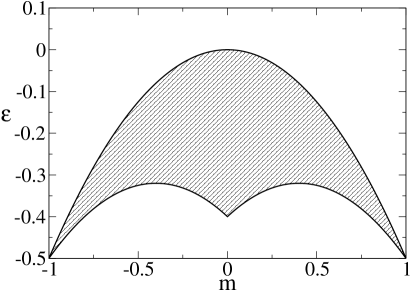
Figure 5: Accessible region in the $(m,\epsilon)$ plane (shaded area) of the Hamiltonian (1) with $K=-0.4$. At low energies, the accessible domain is composed of two disjoint magnetization intervals and at intermediate energies three such intervals exist, yielding ergodicity breaking. At higher energies the three intervals join together and ergodicity is restored.

4 Slow relaxation

In systems with short range interactions the relaxation from a thermodynamically unstable state is typically a fast process. For example, in a magnetic, Ising like system, starting with a magnetically disordered state at a low temperature, where the stable state is the ordered one, the system will locally order in short time. This leads to a domain structure in which the system is divided into magnetically up and down domains of some typical size. The domains forming process is fast in the sense that its characteristic time does not scale with the system size. This domain structure is formed by fluctuations, when a locally ordered region reaches a critical size for which the loss its surface free energy is compensated by the gain in its bulk free energy. This critical size is independent of the system size, leading to a finite relaxation time. Once the domain structure is formed it exhibits a coarsening process in which the domains grow in size while their number is reduced. This process, which is typically slow, eventually leads to the ordered equilibrium state of the system.

This is very different from what happens in systems with strong long range interactions. Here the initial relaxation from a thermodynamically unstable state need not be fast and it could take place over a time scale which diverges with the system size. The reason is that in the case of long range interactions one cannot define a critical size of an ordered domain, since the bulk and surface energies of a domain are of the same order. It is thus of great interest to study relaxation processes in systems with long range interactions and to explore the types of behavior which might be encountered. In principle the relaxation process may depend on the nature and symmetry of the order parameter, say, whether it is discrete, Ising like, or one with a continuous symmetry such as the $XY$ model. It may also depend on the dynamical process, whether it is stochastic or deterministic. In this subsection we briefly review some recent results obtained in studies of the dynamics of some models with long range interactions.

We start by considering the Ising model with long and short range interactions defined in section (2). The relaxation processes in this model have recently been studied [Mukamel et al (2005)]. Since Ising models do not have intrinsic dynamics, the common dynamics one uses in studying them is the Monte Carlo (MC) dynamics, which simulates the stochastic coupling of the model to a thermal bath. If one is interested in studying the dynamics of an isolated system, one has to resort to the microcanonical MC algorithm developed by Creutz  [Creutz (1983)] some time ago. According to this algorithm a demon with energy $E_{d}\geq 0$ is allowed to exchange energy with the system. One starts with a system with energy $E$ and a demon with energy $E_{d}=0$. The dynamics proceeds by selecting a spin at random and attempting to flip it. If, as a result of the flip, the energy of the system is reduced, the flip is carried out and the excess energy is transferred to the demon. On the other hand if the energy of the system increases as a result of the attempted flip, the energy needed is taken from the demon and the move is accepted. In case the demon does not have the necessary energy the move is rejected. After sufficiently long time and for large system size, $N$, the demon’s energy will be distributed according to the Boltzmann distribution $\exp(-E_{d}/k_{B}T)$, where $T$ is the temperature of the system with energy $E$. Thus, by measuring the energy distribution of the demon one obtains the caloric curve of the system. Note that as long as the entropy of the system is an increasing function of its energy, the temperature is positive and the average energy of the demon is finite. The demon’s energy is thus negligibly small compared with the energy of the system, which scales with its size. The energy of the system at any given time is $E-E_{D}$, and it exhibits fluctuations of finite width at energies just below $E$.

In applying the microcanonical MC dynamics to models with long range interactions, one should note that the Boltzmann expression for the energy distribution of the demon is valid only in the large $N$ limit. To next order in $N$ one has

$$P(E_{D})\sim\exp{(-E_{D}/T-E_{D}^{2}/{2C_{V}T^{2}})}~{},$$ (14)

where $C_{V}=O(N)$ is the system’s specific heat. In systems with short range interactions, the specific heat is non-negative and thus the next to leading term in the distribution function is a stabilizing factor which may be neglected for large $N$. On the other hand, in systems with long range interactions, $C_{V}$ may be negative in some regions of the phase diagram, and on the face of it, the next to leading term may destabilize the distribution function. However the next to leading term is small, of order $O(1/N)$, and it is straightforward to argue that as long as the entropy is an increasing function of the energy, the next to leading term does not destabilize the distribution. The Boltzmann distribution for the energy of the demon is thus valid for large $N$.

Using the microcanonical MC algorithm, the dynamics of the model (1) has been studied in detail [Mukamel et al (2005)]. Breaking of ergodicity in the region in the $(K,\epsilon)$ plane where it is expected to take place has been observed.

The microcanonical MC dynamics has also been applied to study the relaxation process of thermodynamically unstable states. It has been found that starting with a zero magnetization state at energies where this state is a local minimum of the entropy, the model relaxes to the equilibrium, magnetically ordered, state on a time scale which diverges with the system size as $\ln N$. The divergence of the relaxation time is a direct result of the long range interactions in the model.

The logarithmic divergence of the relaxation time may be understood by considering the Langevin equation which corresponds to the dynamical process. The equation for the magnetization $m$ is

$$\frac{\partial m}{\partial t}=\frac{\partial s}{\partial m}+\xi(t)\,\,\,,\,\,\,<\xi(t)\xi(t^{\prime})>=D\delta(t-t^{\prime})$$ (15)

where $\xi(t)$ is the usual white noise term. The diffusion constant $D$ scales as $D\sim 1/N$. This can be easily seen by considering the non-interacting case in which the magnetization evolves by pure diffusion where the diffusion constant is known to scale in this form. Since we are interested in the case of a thermodynamically unstable $m=0$ state, which corresponds to a local minimum of the entropy, we may, for simplicity, consider an entropy function of the form

$$s(m)=am^{2}-bm^{4}$$ (16)

with $a$ and $b$ non-negative parameters. In order to analyze the the relaxation process we consider the corresponding Fokker-Planck equation for the probability distribution $P(m,t)$ of the magnetization at time $t$. It takes the form

$$\frac{\partial P(m,t)}{\partial t}=D\frac{\partial^{2}P(m,t)}{\partial m^{2}}-\frac{\partial}{\partial m}\left(\frac{\partial s}{\partial m}P(m,t)\right)\;,$$ (17)

This equation could be viewed as describing the motion of a particle whose coordinate, $m$, carries out an overdamped motion in a potential $-s(m)$ at temperature $T=D$. In order to probe the relaxation process from the $m=0$ state it is sufficient to consider the entropy (16) with $b=0$. With the initial condition for the probability distribution $P(m,0)=\delta(m)$, the large time asymptotic distribution is found to be [Risken (1996)]

$$P(m,t)\sim\exp\left[-\frac{ae^{-at}m^{2}}{D}\right]\,.$$ (18)

This is a Gaussian distribution whose width grows with time. Thus, the relaxation time from the unstable state, $\tau_{us}$, which corresponds to the width reaching a value of $O(1)$, satisfies

$$\tau_{us}\sim-\ln D\sim\ln N~{}.$$ (19)

The logarithmic divergence with $N$ of the relaxation time seems to be independent of the nature of the dynamics. Similar behavior has been found when the model (1) has been studied within the Metropolis-type canonical dynamics at fixed temperature [Mukamel et al (2005)].

The relaxation process from a metastable state (rather than an unstable state discussed above) has been studied rather extensively in the past. Here the entropy has a local maximum at $m=0$, while the global maximum is obtained at some $m\neq 0$. As one would naively expect, the relaxation time from the metastable $m=0$ state, $\tau_{ms}$, is found to grow exponentially with $N$ [Mukamel et al (2005)]

$$\tau_{ms}\sim e^{N\Delta s}~{}.$$ (20)

The entropy barrier corresponding to the non-magnetic state, $\Delta s$, is the difference in entropy between that of the $m=0$ state and the entropy at the local minimum separating it from the stable equilibrium state. Such exponentially long relaxation times are expected to take place independently of the nature of the order parameter or the type of dynamics (whether it is stochastic or deterministic). This has been found in the past in numerous studies of canonical, Metropolis-type dynamics, of the Ising model with mean-field interactions [Griffiths et al (1966)], in deterministic dynamics of the $XY$ model [Antoni et al (2004)] and in models of gravitational systems [Chavanis and Rieutord (2003), Chavanis (2005)].

A different, rather intriguing, type of relaxation process has been found in studies of the Hamiltonian dynamics of the $XY$ model with mean-field interactions [Antoni and Ruffo (1995), Latora et al (1998), Latora et al (1999), Yamaguchi (2003), Yamaguchi et al (2004)]. This model has been termed the Hamiltonian Mean Field (HMF) model. In this model, some non-equilibrium quasi-stationary states have been identified, whose relaxation time grows as a power of the system size, $N$, for some energy interval. These non-equilibrium quasi-stationary states (which become steady states in the thermodynamic limit) exhibit some interesting properties such as anomalous diffusion which have been extensively studied ([Latora et al (1999), Yamaguchi (2003), Yamaguchi et al (2004), Bouchet and Dauxois (2005)]). At other energy intervals the relaxation process has been found to be much faster, with a relaxation time which grows as $\ln N$ [Jain et al (2007)]. In what follows we briefly outline the main results obtained for the HMF model and for some generalizations of it.

The HMF model is defined on a lattice with each site occupied by an $XY$ spin of unit length. The Hamiltonian takes the form

$$H=\sum_{i=1}^{N}\frac{p_{i}^{2}}{2}+\frac{1}{2N}\sum_{i,j=1}^{N}\left[1-\cos(\theta_{i}-\theta_{j})\right]~{},$$ (21)

where $\theta_{i}$ and $p_{i}$ are the phase and momentum of the $i$th particle, respectively. In this model the interaction is mean-field like. The model exhibits a continuous transition at a critical energy $\epsilon_{c}=3/4$ from a paramagnetic state at high energies to a ferromagnetic state at low energies. Within the Hamiltonian dynamics, the equations of motion of the dynamical variables are

$$\frac{d\theta_{i}}{dt}=p_{i}~{},\qquad\qquad\frac{dp_{i}}{dt}=-m_{x}\sin\theta_{i}+m_{y}\cos\theta_{i}~{},$$ (22)

where $m_{x}$ and $m_{y}$ are the components of the magnetization density

$$\vec{m}=\left(\frac{1}{N}\sum_{i=1}^{N}\cos\theta_{i},\frac{1}{N}\sum_{i=1}^{N}\sin\theta_{i}\right)~{}.$$ (23)

The Hamiltonian dynamics obviously conserves both energy and momentum. A typical initial configuration for the non-magnetic state is taken as the one where the phase variables are uniformly and independently distributed in the interval $\theta_{i}\in[-\pi,\pi]$. A particularly interesting case is that where the initial distribution of the momenta is uniform in an interval $[-p_{0},p_{0}]$. This has been termed the waterbag distribution. For such phase and momentum distributions the initial energy density is given by $\epsilon=p_{0}^{2}/6-1/2$.

Extensive numerical studies of the relaxation of the non-magnetic state with the waterbag initial distribution have been carried out. It has been found that at an energy interval just below $\epsilon_{c}$ this state is quasi-stationary, in the sense that the magnetization fluctuates around its initial value for some time $\tau_{qs}$ before it switches to the non-vanishing equilibrium value. This characteristic time has been found to scale as [Yamaguchi (2003), Yamaguchi et al (2004)]

$$\tau_{qs}\sim N^{\gamma}$$ (24)

with $\gamma\simeq 1.7$.

A very useful insight into the dynamics of the HMF model is provided by analyzing the evolution of the probability distribution of the phase and momentum variables, $f(\theta,p,t)$, within the Vlasov equation approach [Yamaguchi et al (2004)]. It has been found that in the energy interval $\epsilon^{*}<\epsilon<\epsilon_{c}$, with $\epsilon^{*}=7/12$, the waterbag distribution is linearly stable. It is unstable for $\epsilon<\epsilon^{*}$. In this interval the following growth law for the magnetization $m=\sqrt{m_{x}^{2}+m_{y}^{2}}~{}$ has been found [Jain et al (2007)]:

$$m(t)\sim\frac{1}{\sqrt{N}}e^{\Omega t}~{},$$ (25)

where

$$\Omega=\sqrt{6(\epsilon^{*}-\epsilon)}~{}.$$ (26)

The robustness of the quasi-stationary state to various perturbations has been explored in a number of studies. The anisotropic HMF model has recently been shown to exhibit similar relaxation processes as the HMF model itself [Jain et al (2007)]. The anisotropic HMF model is defined by the Hamiltonian

$$H=\sum_{i=1}^{N}\frac{p_{i}^{2}}{2}+\frac{1}{2N}\sum_{i,j=1}^{N}\left[1-\cos(\theta_{i}-\theta_{j})\right]-\frac{D}{2N}\left[\sum_{i=1}^{N}\cos\theta_{i}\right]^{2}~{},$$ (27)

where the anisotropy term with $D>0$ represents global coupling and favors order along the $x$ direction. The model exhibits a transition from magnetically disordered to a magnetically ordered state along the $x$ direction at a critical energy $\epsilon_{c}=(3+D)/4$. An analysis of the Vlasov equation corresponding to this model shows that as in the isotropic case, the waterbag initial condition is stable for $\epsilon^{*}<\epsilon<\epsilon_{c}$, where $\epsilon^{*}=(7+D)/12$. In this energy interval a quasi-stationary state has been observed numerically, with a power law behavior (24) of the relaxation time. The exponent $\gamma$ does not seem to change with the anisotropy parameter. Logarithmic growth in $N$ of the relaxation time is found for $\epsilon<\epsilon^{*}$. A model with local, on site anisotropy term has also been analyzed along the same lines [Jain et al (2007)]. The model is defined by the Hamiltonian

$$H=\frac{1}{2}\sum_{i=1}^{N}p_{i}^{2}+\frac{1}{2N}\sum_{i,j=1}^{N}(1-\cos(\theta_{i}-\theta_{j}))+W\sum_{i=1}^{N}\cos^{2}\theta_{i}~{}.$$ (28)

Here, too, both types of behavior have been found.

Other extensions of the HMF model include the addition of short range, nearest neighbor coupling to the Hamiltonian [Campa et al (2006)], and coupling of the HMF model to a thermal bath, making the dynamics stochastic [Baldovin and Orlandini (2006)]. In both cases quasi-stationarity is observed with a power law growth of the relaxation time (24) with an exponent $\gamma$ which seems to vary with the interaction parameters of the models.

3 Weak Long Range Interactions

In this section we consider weak long range interactions, where $0<\sigma<\sigma_{c}(d)$. Systems with such interactions are additive and thus the special features found for strong long range interactions do not take place. However, as discussed in the Introduction, due to the long range correlations which are built in the vicinity of phase transitions weak long range interactions are expected to modify their thermodynamic properties. Systems with weak long range interactions have been extensively studied over the last four decades. Much is known about the collective behavior of these systems, the mechanism by which they induce long range order in low dimensions and the their critical behavior at continuous phase transitions. In this Section we discuss two features of these interactions: long range order in $1d$ models, and the upper critical dimension above which the critical exponents of a second order phase transition are given by the Landau or mean-field exponents.

1 Long Range Order in a one dimensional Ising Model

Over 70 years ago Peierls [Peierls ( 1923), Peierls ( 1935)] and Landau [Landau ( 1937), Landau and Lifshitz (1969)] concluded that long range order (or spontaneous symmetry breaking) does not take place in $1d$ systems with short range interactions at finite temperatures. This may be easily argued by considering the $1d$ Ising model with nearest neighbor interaction

$$H=-J\sum_{i=1}^{N-1}S_{i}S_{i+1}$$ (29)

where $J>0$ is a ferromagnetic coupling. The ground state of the model is ferromagnetic with all spins parallel, say, in the up direction. consider now an excitation where all spins in a segment of length $n$ are flipped down. The energy cost of this excitation is $4J$, and is independent of the length $n$. On the other hand the entropy of this excitation is $\ln N$, as the segment can be located at any point on the lattice. The free energy cost of the excitation is thus

$$\Delta F=4J-T\ln N$$ (30)

which for sufficiently large $N$ is negative at any given temperature $T>0$. Thus at any finite temperature and in the thermodynamic limit, more excitations with arbitrarily large $n$ are generation and the ferromagnetic long range order of the $T=0$ ground state is destroyed.

The non-existence of phase transitions in $1d$ models with short range interactions can also be demonstrated by considering the transfer matrix of the model. Since due to the short range nature of the interactions the matrix is of finite order, and since all the matrix elements are positive, the Perron-Frobenius theorem guarantees that its largest eigenvalue is positive and non-degenerate [Bellman (1970), Ninio (1976)]. However, for a transition to take place the largest eigenvalue has to become degenerate. Thus no transition takes place.

The argument presented above for the $1d$ case does not apply for the Ising model in higher dimensions. The reason is that the energy cost of a flipped droplet of linear size $R$ scales as the surface area of the droplet, $R^{d-1}$. Generating large droplets is thus energetically costly, and long range order can be maintained at sufficiently low temperatures. From the dynamical point of view the increase of the energy cost with the droplet size means that there is a driving force on the droplet to shrink, and thus while droplets are spontaneously generated at finite temperatures, they tend to decrease in size with time. At low temperatures, where the rate at which droplets are generated are small, droplets do not have a chance to join together and flip the magnetization of the initial ground state before they shrink and disappear. Thus long range order is preserved in the long time limit. This is in contrast with the $1d$ case, where the energy cost of a droplet is independent of its size, and there is no driving force on a droplet to shrink.

In 1969, Dyson introduced an Ising model with a pair-wise coupling which decreases algebraically with the distance between the spins [Dyson ( 1969a), Dyson ( 1969b)]. He demonstrated that depending on the power law of the coupling, the model may exhibit a phase transition and long range order. The Hamiltonian of the Dyson model is

$$H=-\sum_{i,j}J(j)S_{i}S_{i+j}~{},$$ (31)

with

$$J(j)=\frac{J}{j^{1+\sigma}}~{}.$$ (32)

where $J>0$ is a constant. It has been shown that for weak long range interactions, namely for $0<\sigma<\sigma_{c}(d=1)=1$, the model exhibits long range order. The fact that $\sigma_{c}(d=1)=1$ will be discussed in what follows.

To argue for the existence of a phase transition in this model we apply the argument given above for the case of short range interactions to the Hamiltonian (31). To this end we take the ferromagnetic ground state of the model and consider the excitation energy of a state in which, say, the leftmost $n$ spins are flipped. The energy of this excitation is

$$E=2J\sum_{k=1}^{n}\sum_{j=l-k+1}^{N-k}\frac{1}{j^{1+\sigma}}~{}.$$ (33)

In order to estimate this energy we replace the sums by integrals,

$$E\sim 2J\int_{1}^{n}dy\int_{n-k+1}^{N-y}dx\frac{1}{x^{1+\sigma}}~{}.$$ (34)

The integrals may be readily evaluated to yield

$$E\sim-\frac{2J}{\sigma}nN^{-\sigma}+\frac{2J}{\sigma(1-\sigma)}(n^{1-\sigma}-1)~{}.$$ (35)

For $0<\sigma<1$ the first term in (35) vanishes in the thermodynamic limit and the excitation energy increases with the length of the droplet as $n^{1-\sigma}$. Therefore, large droplets tend to shrink in size. This is similar to the behavior of droplets in models with short range interactions in dimension higher than one. Thus at low enough temperatures, the model is expected to exhibit spontaneous symmetry breaking. On the other hand for $\sigma>1$ the energy of a droplet is bounded, approaching $2J/\sigma(\sigma-1)$ in the large $n$ limit. As in the case of the short range model, no spontaneous symmetry breaking is expected to take place here. It is interesting to note that for the case of strong long range interactions, namely for $\sigma<0$, the excitation energy increases with the system size as $N^{-\sigma}$ and the energy is super- extensive.

The Dyson model has been a subject of extensive studies over the years. A particular point of interest is its behavior at the borderline case $\sigma=1$, where logarithmic corrections to the power law decay are significant . Also, as will be discussed in the following subsection, the critical exponents of the model are expected to be mean-field like for $0<\sigma<1/2$, see, for example, [Luijten and Blöte ( 1997), Monroe (1998)].

2 Upper Critical Dimension

Perhaps the simplest approach for studying phase transitions in a given system is provided by the Landau theory [Landau and Lifshitz (1969)]. In this theory one first identifies the order parameter of the transition, say the local magnetization, $m$, in the case of a magnetic transition. One then uses the symmetry properties of the order parameter, expand the free energy in powers of the order parameter and determine its equilibrium value by minimizing the free energy. In the case of a single component, Ising like, magnetic transition, the free energy per unit volume $f$ takes the form

$$f=\frac{1}{2}tm^{2}+\frac{1}{4}um^{4}+O(m^{6})~{},$$ (36)

where $t$ and $u>0$ are phenomenological parameters. The fact that only even powers of $m$ appear in this expansion is a result of the up-down symmetry of the magnetic order parameter. The equilibrium magnetization $m$ is found by minimizing this free energy. This theory yields a phase transition at $t=0$, with $m=0$ for $t>0$ and $m=\sqrt{-t/u}$ for $t<0$. Thus the parameter $t$ may be taken as temperature dependent with $t\propto(T-T_{c})/T_{c}$ close to the critical temperature $T_{C}$. Below the transition the order parameter grows as $m\propto(-t)^{\beta}$, with the order parameter critical exponent $\beta=1/2$. Similarly, one can obtain the other critical exponents associated with the transition. For example the free energy per unit volume, $f$, of the model (36) is $0$ for $t>0$ and $-t^{2}/4u$ for $t<0$. Thus the specific heat per unit volume, $C=-T\partial^{2}f/\partial T^{2}$, exhibits a discontinuity at the transition. The critical exponent $\alpha$ associated with the specific heat singularity, $C\propto t^{-\alpha}$, is thus $\alpha=0$ within the Landau theory. Other critical exponent, corresponding to other thermodynamic quantities such as the magnetic susceptibility, correlation function etc. can be easily calculated in a similar fashion. Within the Landau theory, the coefficients in the free energy (36) are taken as phenomenological parameters. For any given microscopic model, these coefficients may be calculated using the mean-field theory, in which fluctuations of the order parameter are neglected.

Theories which neglect fluctuations of the order parameter usually yield the exact free energy of the model only in the limit of infinite dimension. However one can show that the mean-field, or the Landau theory, yield the correct critical exponents above a critical dimension, which for systems with short range interactions is $d_{c}=4$. This dimension is referred to as the upper critical dimension of the model. For $d<d_{c}$, the critical exponents become $d$-dependent, and the fluctuations of the order parameter need to be properly taken care of. This is usually done, for example, by applying renormalization group techniques. For reviews see, for example [Fisher ( 1974), Fisher ( 1998)]. Long range interactions tend to suppress fluctuations. It is thus expected that long range interactions should result in a smaller critical dimension, $d_{c}(\sigma)$, which could be a function of the interaction parameter $\sigma$. They can also modify the critical exponents below the critical dimension, see [Fisher et al (1972)]. The case of dipolar interactions is of particular interest. For these anisotropic interactions the upper critical dimension remains $d_{c}=4$, however the critical exponents at dimensions below $4$ are modified by the long range nature of the interaction, see [Aharony and Fisher ( 1974)].

In this Section we consider the upper critical dimension of systems with weak long range interactions. We first analyze the case of short range interactions, and then extend the analysis to models with long range interactions. To this end one should extend the Landau theory to allow for fluctuations of the order parameter, and examine their behavior close to the transition. A convenient and fruitful starting point for this analysis is provided by constructing the coarse grained effective Hamiltonian of the system. This Hamiltonian, referred to as the Landau-Ginzburg model, is expressed in terms of the long wavelength degrees of freedom, and is obtained by averaging over the short wavelength ones. For any given system, this model can be derived phenomenologically using the symmetry properties of the order parameter involved in the transition. For example, for systems with a single component, Ising-like, order parameter, say, the magnetization, the effective Hamiltonian is expressed in terms of the local coarse grained magnetization $m({\bf r})$. For systems with short range interactions the Hamiltonian takes the form

$$\beta H=\int d^{d}r[\frac{1}{2}tm^{2}+\frac{1}{4}um^{4}+\frac{1}{2}(\nabla m)^{2}]~{},$$ (37)

where $t$ and $u>0$ are phenomenological parameters, as in the Landau theory, and $d$ is the spatial dimension. It is obtained as an expansion in the small order parameter $m$, using the up-down symmetry of the microscopic interactions, noting that short range local interactions result in a long wavelength gradient term in the energy, of the form $(\nabla m)^{2}$. The partition sum, $Z$, corresponding to this Hamiltonian is obtained by carrying out the functional integral over all magnetization profiles $m({\bf r})$,

$$Z=\int D[m(\vec{r})]e^{-\beta H}~{}.$$ (38)

When spatial fluctuations of the order parameter are neglected, the model is reduced to the Landau theory discussed above.

Before demonstrating that the upper critical dimension of the model (37) is $d_{c}=4$, we consider the model at $t>0$ and evaluate the fluctuations of the order parameter around its average value $<m>=0$. To this end we express the effective Hamiltonian in terms of the Fourier modes of the order parameter,

$$m({\bf q})=\int d^{d}re^{i{\bf q}\cdot{\bf r}}m({\bf r})~{}.$$ (39)

In terms of these modes one has

$$m({\bf r})=\frac{1}{V}\sum_{{\bf q}}e^{-i{\bf q}\cdot{\bf r}}m({\bf q})~{},$$ (40)

and

$$\int m^{2}({\bf r})=\frac{1}{V}\sum_{{\bf q}}m({\bf q})m(-{\bf q})$$ (41)

Neglecting the fourth order terms in the effective Hamiltonian (37) one is left with a Gaussian model which can be expressed in terms of the Fourier modes as

$$\beta H=\frac{1}{2V}\sum_{{\bf q}}(t+q^{2})m({\bf q})m(-{{\bf q}})~{}.$$ (42)

In the limit $V\rightarrow\infty$ the sum can be expressed as an integral

$$\beta H=\frac{1}{2(2\pi)^{d}}\int d^{d}q(t+q^{2})m({\bf q})m(-{\bf q})~{}.$$ (43)

To calculate the two-point order parameter correlation function, one first evaluates the average amplitudes of the Fourier modes using the Gaussian Hamiltonian (42),

$$<m({\bf q})m({\bf q^{\prime}})>=\frac{V}{t+q^{2}}\delta_{{\bf q},-{\bf q^{\prime}}}~{}.$$ (44)

The two-point correlation function is then given by

$$<m({\bf r})m({\bf r^{\prime}})>=\frac{1}{V}\sum_{{\bf q}}\frac{1}{t+q^{2}}e^{-i{\bf q}{\bf(r-r^{\prime})}}~{},$$ (45)

which in the $V\rightarrow\infty$ limit becomes

$$<m({\bf r})m({\bf r^{\prime}})>=\frac{1}{(2\pi)^{d}}\int d^{d}q\frac{e^{-i{\bf q}{\bf(r-r^{\prime})}}}{t+q^{2}}~{}.$$ (46)

Scaling ${\bf q}$ by $\sqrt{t}$ the integral (46) implies that the correlation function can be expressed in terms of a correlation length

$$\xi=t^{1/2}~{},$$ (47)

which diverges at the critical point with an exponent $\nu=1/2$. It is easy to verify that at distances larger than $\xi$ the correlation function decays exponentially with the distance as $e^{-{\bf|r-r^{\prime}|}/\xi}$ with a sub-leading power law correction.

The Landau Ginzburg effective Hamiltonian (37) may be used to calculate the local fluctuations of the order parameter, on a coarse grained scale of of linear size $\xi$. From (41) and (44) it follows that

$$<m^{2}({\bf r})>\equiv\frac{1}{V}\int d^{d}rm^{2}({\bf r})=\frac{1}{V}\sum_{{\bf q}}\frac{1}{t+q^{2}}~{}.$$ (48)

Taking now the limit $V\rightarrow\infty$, and integrating over modes with a wavelength bigger than the correlation length $\xi$, namely $0<q<\xi^{-1}=\sqrt{t}$ one finds

$$<m^{2}({\bf r})>=\int_{q<{\sqrt{t}}}\frac{d^{d}q}{(2\pi)^{d}}\frac{1}{t+q^{2}}~{}\propto~{}t^{\frac{d}{2}-1}~{}.$$ (49)

In the Landau theory, the fluctuations of the order parameter have been neglected. To check the validity of this assumption, or alternatively, to check at which dimensions this assumption is valid, we consider the fluctuations below the critical point ($t<0$). Let

$$m_{0}=\sqrt{-\frac{t}{u}}$$ (50)

be the order parameter at $t<0$. To calculate the fluctuations of the order parameter we consider small local deviations $m({\bf r})=m_{0}+\delta m({\bf r})$ around the average value. To second order in $\delta m({\bf r})$ the effective Landau-Ginzburg Hamiltonian is

$$\beta H=\frac{1}{2}(t+3um_{0}^{2})(\delta m({\bf r}))^{2}+\frac{1}{2}(\nabla\delta m({\bf r}))^{2}~{},$$ (51)

which, after using (50), becomes

$$\beta H=|t|(\delta m({\bf r}))^{2}+\frac{1}{2}(\nabla\delta m({\bf r}))^{2}~{}.$$ (52)

Thus the fluctuations of the order parameter around their average value below the transition are controlled by a similar effective Hamiltonian as the fluctuations of the order parameter above $T_{c}$. It therefore follows from (49) that

$$<\delta m^{2}({\bf r})>~{}\propto~{}|t|^{\frac{d}{2}-1}$$ (53)

For the Landau theory to be self consistent near the transition one requires that the fluctuations of the order parameter are negligibly small compared with the order parameter, namely,

$$<\delta m^{2}({\bf r})>~{}\ll~{}m_{0}^{2}~{}.$$ (54)

This amounts to

$$|t|^{\frac{d}{2}-1}~{}\ll~{}|t|~{},$$ (55)

which is satisfied for mall $t$ as long as

$$d>d_{c}=4~{}.$$ (56)

This analysis suggests that in systems with short range interactions, for which the Landau-Ginzburg effective Hamiltonian (37) applies, the fluctuations of the order parameter are negligibly small, and the critical exponents corresponding to the transition are those given by the Landau theory. In dimensions less than $4$ the inequality (55) could be satisfied only away from the critical point $|t|>|t_{G}|$, where $t_{G}$ defines the Ginzburg temperature interval. This interval depends on the amplitudes of the power laws appearing in (55), which can vary from one system to another. This is known as the Ginzburg criterion [Ginzburg ( 1960), Hohenberg ( 1968), Als-Nielsen and Birgeneau ( 1977)]. According to this criterion the true critical exponents of a system in, say, dimension $d=3$, can be observed only at a temperature interval $|t|<|t_{G}|$. Outside this interval, one should expect a crossover of the critical exponents to those of the Landau theory.

So far we discussed the upper critical dimension of a generic critical point of a system with short range interactions. Let us now examine how this analysis is modified when one considers weak long range interactions. For such systems the Landau-Ginzburg effective Hamiltonian takes the form

$$\beta H=\int d^{d}r[\frac{1}{2}tm^{2}+\frac{1}{4}um^{4}]+\int d^{d}r~{}d^{d}r^{\prime}m({\bf r})m({\bf r^{\prime}})\frac{1}{|{\bf r-r^{\prime}}|^{d+\sigma}}~{},$$ (57)

where the second integral yields the contribution of the long range interaction to the energy. In terms of the Fourier components of the order parameter this integral may be expressed as

$$\frac{1}{V}\sum_{{\bf q}}m({\bf q})m({-\bf q})\int d^{d}R\frac{e^{-i{\bf q}\cdot{\bf R}}}{R^{d+\sigma}}~{}.$$ (58)

To leading order in $q$ the Fourier transform of the long range potential is of the form $a+bq^{\sigma}$, where $a$ and $b$ are constants. Note, though, that for integer values of $\sigma$ a logarithmic correction to this form is present. For $\sigma=2$ it becomes $a+bq^{2}\ln q$. These logarithmic corrections do not affect the considerations which will be presented below. Thus the Landau-Ginzburg effective Hamiltonian is

$$\beta H=\frac{1}{2V}\sum_{{\bf q}}(\bar{t}+bq^{\sigma}+q^{2})m({\bf q})m(-{{\bf q}})~{},$$ (59)

where $\bar{t}=t+a$. The $q^{2}$ term results from short range interactions which are always present in the system.

It is straightforward to repeat the above analysis for the upper critical dimension in systems with short range interaction and extend it to the case of weak long range interactions. For $\sigma>2$ the $q^{\sigma}$ term in (59) is dominated by the $q^{2}$ term and may thus be neglected. One is then back to the model corresponding to short range interactions and the upper critical dimension is $d_{c}=4$. On the other hand for $0<\sigma<2$ the dominant term is $q^{\sigma}$. The correlation length in this case diverges as

$$\xi~{}\propto~{}|\bar{t}|^{-1/\sigma}~{}.$$ (60)

The order parameter fluctuations satisfy

$$<(\delta m({\bf r}))^{2}>=\int_{q<1/\xi}\frac{d^{d}q}{(2\pi)^{d}}\frac{1}{2|\bar{t}|+q^{\sigma}}~{}\propto~{}|\bar{t}|^{d/\sigma-1}~{}.$$ (61)

Requiring that the fluctuations are much smaller than the order parameter (54),

$$|\bar{t}|^{d/\sigma-1}~{}\ll~{}|\bar{t}|~{},$$ (62)

one concludes that fluctuations may be neglected as long as

$$d>d_{c}=2\sigma~{}.$$ (63)

Alternatively, this implies that in $d<4$ dimensions there exists a critical $\sigma$

$$\sigma_{c}(d)=\frac{d}{2}$$ (64)

such that for $0<\sigma<\sigma_{c}(d)$ the critical exponents are mean-field like. For $\sigma_{c}(d)<\sigma<2$ the critical exponents are affected by the long range nature of the interaction and they become $\sigma$ dependent, see, for example, [Fisher et al (1972)]. For $\sigma>2$ the critical exponents become those of short range interactions. Applied to the Dyson model discussed in Section 1, these results suggest that in $1d$ the critical exponents of the model are mean-field like for $0<\sigma<1/2$, and become of long range type for $1/2<\sigma<1$. For $\sigma>1$ the interaction is effectively short range and no transition takes place.

The results of this analysis are presented in Fig. (6), where the type of critical behavior in various regions of the $(d,\sigma)$ plane is indicated.

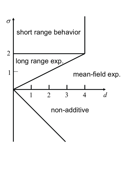
Figure 6: The $(d,\sigma)$ phase diagram, where the type of critical behavior in various regions in this plane is indicated. The system is non-additive with strong long range interactions at $d\leq\sigma\leq 0$. For $\sigma>0$, the critical exponents can be either mean-field, sort range like or characteristic of the long range interactions depending on $\sigma$ and $d$. Note that in the case $\sigma>2$, no phase transition takes place for $d\leq 1$.

4 Long Range Correlations in Non-equilibrium Driven Systems

As discussed in the Introduction, steady states of driven systems are expected to exhibit long range correlations when the dynamics involves one or more conserved variables. This takes place even though the dynamics is local, with transition rates which depend only on the local microscopic configuration of the dynamical variable. Such long range correlations have been shown to lead to phase transitions and long range order in a number of one dimensional models. For reviews on steady state properties of driven models see, for example, [Schmittmann and Zia (1995), Schütz (2001), Derrida (2007), Mukamel (2000)]. Features which are characteristic of strong long range interactions, such as inequivalence of ensembles, have been reported in some cases [Grosskinsky and Schütz (2008)]. In this Section we discuss a particular model, the $ABC$ model, introduced by Evans and co-workers [Evans et al (1998a), Evans et al (1998b)] which exhibits spontaneous symmetry breaking and for which such correlations can be explicitly demonstrated. Moreover, for particular parameters defining this model, its dynamics obey detailed balance. For this choice of the parameters the steady state becomes an equilibrium state, which can be expressed in terms of an effective Hamiltonian. This Hamiltonian has been explicitly expressed in terms of the dynamical variables of the model, and shown to display strong long range interactions.

The model is defined on a $1d$ lattice of length $N$ with periodic boundary conditions. Each site is occupied by either an $A$, $B$, or $C$ particle. The evolution is governed by random sequential dynamics defined as follows: at each time step two neighboring sites are chosen randomly and the particles of these sites are exchanged according to the following rates

(65)

The rates are cyclic in $A$, $B$ and $C$ and conserve the number of particles of each type $N_{A},N_{B}$ and $N_{C}$, respectively.

For $q=1$ the particles undergo symmetric diffusion and the system is disordered. This is expected since this is an equilibrium steady state. However for $q\neq 1$ the particle exchange rates are biased. We will show that in this case the system evolves into a phase separated state in the thermodynamic limit.

To be specific we take $q<1$, although the analysis may trivially be extended for any $q\neq 1$. In this case the bias drives, say, an $A$ particle to move to the left inside a $B$ domain, and to the right inside a $C$ domain. Therefore, starting with an arbitrary initial configuration, the system reaches after a relatively short transient time a state of the type $\ldots AABBCCAAAB\ldots$ in which $A,B$ and $C$ domains are located to the right of $C$, $A$ and $B$ domains, respectively. Due to the bias $q$, the domain walls $\ldots AB\ldots$, $\ldots BC\ldots$, and $\ldots CA\ldots$, are stable, and configurations of this type are long-lived. In fact, the domains in these configurations diffuse into each other and coarsen on a time scale of the order of $q^{-l}$, where $l$ is a typical domain size in the system. This leads to the growth of the typical domain size as $(\ln t)/|\ln q|$. Eventually the system phase separates into three domains of the different species of the form $A\ldots AB\ldots BC\ldots C$. A finite system does not stay in such a state indefinitely. For example, the $A$ domain breaks up into smaller domains in a time of order $q^{-min\{N_{B},N_{C}\}}$. In the thermodynamic limit, however, when the density of each type of particle is non vanishing, the time scale for the break up of extensive domains diverges and we expect the system to phase separate. Generically the system supports particle currents in the steady state. This can be seen by considering, say, the $A$ domain in the phase separated state. The rates at which an $A$ particle traverses a $B$ ($C$) domain to the right (left) is of the order of $q^{N_{B}}$ ($q^{N_{C}}$). The net current is then of the order of $q^{N_{B}}-q^{N_{C}}$, vanishing exponentially with $N$. This simple argument suggests that for the special case $N_{A}=N_{B}=N_{C}$ the current is zero for any system size.

The special case of equal densities $N_{A}=N_{B}=N_{C}$ provide very interesting insight into the mechanism leading to phase separation. We thus consider it in some detail. Examining the dynamics for these densities, one finds that it obeys detailed balance with respect to some distribution function. Thus in this case the model is in fact in thermal equilibrium. It turns out however that although the dynamics of the model is local the effective Hamiltonian corresponding to the steady state distribution has long range interactions, and may thus lead to phase separation. This particular mechanism is specific for equal densities. However the dynamical argument for phase separation given above is more general, and is valid for unequal densities as well.

In order to specify the distribution function for equal densities, we define a local occupation variable $\{X_{i}\}=\{A_{i},B_{i},C_{i}\}$, where $A_{i}$, $B_{i}$ and $C_{i}$ are equal to one if site $i$ is occupied by particle $A$, $B$ or $C$ respectively and zero otherwise. The probability of finding the system in a configuration $\{X_{i}\}$ is given by

$$W_{N}(\{X_{i}\})=Z_{N}^{-1}q^{{H}(\{X_{i}\})}.$$ (66)

where $H$ is the Hamiltonian

$${H}(\{X_{i}\})=\sum_{i=1}^{N-1}\sum_{k=i+1}^{N}(C_{i}B_{k}+A_{i}C_{k}+B_{i}A_{k})-(N/3)^{2},$$ (67)

and the partition sum is given by $Z_{N}=\sum q^{{H}(\{X_{i}\})}$. In this Hamiltonian, the site $i=1$ can be arbitrarily chosen as one of the sites on the ring. It is easy to see that the Hamiltonian does not depend on this choice and the Hamiltonian is translationally invariant as expected. The interactions in this Hamiltonian are strong long range interactions, where the the strength of the interaction between two sites is independent of their distance. This corresponds to $\sigma=-1$ in the notation used in these Notes. The Hamiltonian is thus super-extensive, and the energy of macroscopic excitations scale as $N^{2}$.

In order to verify that the dynamics (65) obeys detailed balance with respect to the distribution function (66,67) it is useful to note that the energy of a given configuration may be evaluated in an alternate way. Consider the fully phase separated state

$$A\ldots AB\ldots BC\ldots C$$ (68)

The energy of this configuration is $E=0$, and, together with its translationally relates configurations, they constitute the $N-$fold degenerate ground state of the system. We now note that nearest neighbour (nn) exchanges $AB\rightarrow BA,BC\rightarrow CB$ and $CA\rightarrow AC$ cost one unit of energy each, while the reverse exchanges result in an energy gain of one unit. The energy of an arbitrary configuration may thus be evaluated by starting with the ground state and performing nn exchanges until the configuration is reached, keeping track of the energy changes at each step of the way. This procedure for obtaining the energy is self consistent only when the densities of the three species are equal. To examine self consistency of this procedure consider, for example, the ground state (68), and move the leftmost particle $A$ to the right by a series of nn exchanges until it reaches the right end of the system. Due to translational invariance, the resulting configuration should have the same energy as (68), namely $E=0$. On the other hand the energy of the resulting configuration is $E=N_{B}-N_{C}$ since any exchange with a $B$ particle yields a cost of one unit while an exchange with a $C$ particle yields a gain of one unit of energy. Therefore for self consistency the two densities $N_{B}$ and $N_{C}$ have to be equal, and similarly, they have to be equal to $N_{A}$.

The Hamiltonian (67) may be used to calculate steady state averages corresponding to the dynamics (65). We start by an outline of the calculation of the free energy. Consider a ground state of the system (68). The low lying excitations around this ground state are obtained by exchanging nn pairs of particles around each of the three domain walls. Let us first examine excitations which are localized around one of the walls, say, $AB$. An excitation can be formed by one or more $B$ particles moving into the $A$ domain (equivalently $A$ particles moving into the $B$ domain). A moving $B$ particle may be considered as a walker. The energy of the system increases linearly with the distance traveled by the walker inside the $A$ domain. An excitation of energy $m$ at the $AB$ boundary is formed by $j$ walkers passing a total distance of $m$. Hence, the total number of states of energy $m$ at the $AB$ boundary is equal to the number of ways, $P(m)$, of partitioning an integer $m$ into a sum of (positive) integers. This and related functions have been extensively studied in the mathematical literature over many years. Although no explicit general formula for $P(m)$ is available, its asymptotic form for large $m$ is known [Andrews (1976)]

$$P(m)\simeq\frac{1}{4m\sqrt{3}}\exp{(\pi(2/3)^{1/2}\ m^{1/2})}.$$ (69)

Also, a well known result attributed to Euler yields the generating function

$$Y=\sum_{m=0}^{\infty}q^{m}P(m)=\frac{1}{(q)_{\infty}},$$ (70)

where

$$(q)_{\infty}=\lim_{n\rightarrow\infty}(1-q)(1-q^{2})\ldots(1-q^{n}).$$ (71)

This result may be extended to obtain the partition sum $Z_{N}$ of the full model. In the limit of large $N$ the three domain walls basically do not interact. It has been shown that excitations around the different domain boundaries contribute additively to the energy spectrum [Evans et al (1998b)]. As a result in the thermodynamic limit the partition sum takes the form

$$Z_{N}=N/[(q)_{\infty}]^{3},$$ (72)

where the multiplicative factor $N$ results from the $N-$fold degeneracy of the ground state and the cubic power is related to the three independent excitation spectra associated with the three domain walls.

It is of interest to note that the partition sum is linear and not exponential in $N$, as is the case for systems with short range interactions, leading to a non-extensive free energy. Since the energetic cost of macroscopic excitations is of order $N^{2}$ they are suppressed, and the equilibrium state is determined by the ground state and some local excitations around it.

Whether or not a system has long-range order in the steady state can be found by studying the decay of two-point density correlation functions. For example the probability of finding an $A$ particle at site $i$ and a $B$ particle at site $j$ is,

$$\langle A_{i}B_{j}\rangle=\frac{1}{Z_{N}}\sum_{\{X_{k}\}}A_{i}B_{j}~{}q^{{H}(\{X_{k}\})},$$ (73)

where the summation is over all configurations $\{X_{k}\}$ in which $N_{A}=N_{B}=N_{C}$. Due to symmetry many of the correlation functions will be the same, for example $\langle A_{i}A_{j}\rangle=\langle B_{i}B_{j}\rangle=\langle C_{i}C_{j}\rangle$. A sufficient condition for the existence of phase separation is

$$\lim_{r\rightarrow\infty}~{}\lim_{N\rightarrow\infty}(\langle A_{1}A_{r}\rangle-\langle A_{1}\rangle\langle A_{r}\rangle)>0.$$ (74)

Since $\langle A_{i}\rangle=1/3$ we wish to show that $\lim_{r\rightarrow\infty}~{}\lim_{N\rightarrow\infty}\langle A_{1}A_{r}\rangle>1/9$. In fact it can be shown [Evans et al (1998b)] that for any given $r$ and for sufficiently large $N$,

$$\langle A_{1}A_{r}\rangle=1/3-{O}(r/N).$$ (75)

This result not only demonstrates that there is phase separation, but also that each of the domains is pure. Namely the probability of finding a particle a large distance inside a domain of particles of another type is vanishingly small in the thermodynamic limit.

The $ABC$ model exhibits phase separation and long range order as long as $q\neq 1$. The parameter $q$ is in fact a temperature variable in the case of equal densities, with $\beta=-\ln q$ as can be seen from (66). Thus the model leads to a phase separated state at any finite temperature. A very interesting limit is that of $q\rightarrow 1$, which amount to taking the infinite temperature limit. To probe this limit Clincy and co-workers [Clincy et al (2003)] studied the case $q=e^{-\beta/N}$. This amount to either scaling the temperature by N or alternatively scaling the Hamiltonian (67) by $1/N$, as is done by the Kac prescription. It has been shown that in this case the model exhibits a phase transition at inverse temperature $\beta_{c}=2\pi\sqrt{3}$, where the system is homogeneous at high temperatures and phase separated at low temperatures.

The analysis of the $ABC$ model presented in this section indicates that rather generally, one should expect features which are characteristic of long range interactions, to show up in steady states of driven systems. In the $ABC$ model, for equal densities where the effective Hamiltonian governing the steady state can be explicitly written, the interactions are found to be of strong long range (in fact mean-field) nature. By continuity, this is expected to hold even for the non-equal densities case, where no effective interaction can be written. It is of interest to explore in more detail steady state properties of driven systems within the framework of systems with long range interactions outlined above.

5 Summary

In these Notes some properties of systems with long range interactions have been discussed. Two broad classes can be identified in systems with pairwise interactions which decay as $1/r^{d+\sigma}$ at large distances $r$. Those with $-d\leq\sigma\leq 0$, which we term ”strong” long range interactions and those with $0<\sigma\leq\sigma_{c}(d)$ which are termed ”weak” long range interactions. Here $\sigma_{c}(d)=2$ for $d\geq 4$ and $\sigma_{c}(d)=d/2$ for $d<4$. Some thermodynamic and dynamical features which are characteristic of these two classes have been discussed and demonstrated in representative models.

Systems with strong LRI are non-additive and as a result they do not share many of the common features of systems with short range interactions. In particular, the various ensembles need not be equivalent, the microcanonical specific heat can be negative and temperature discontinuity can take place as the energy of the system is varied. These systems also display distinct dynamical behavior, with slow relaxation processes where the characteristic relaxation time diverges with the system size. In addition they are found to exhibit breaking of ergodicity which is induced by the long range nature of the interaction. Some general considerations arguing that such phenomena should take place have been presented. Simple models (the Ising model with long and short range interactions and the XY model) have been analyzed, where these features are explicitly demonstrated. While the models are mean-field like with $\sigma=-d$, the characteristic features they display are expected to hold in the broader class of systems with $-d\leq\sigma\leq 0$.

Systems with weak LRI are additive, and therefore the general statistical mechanical framework of systems with short range interactions applies here as well. However, near phase transitions, where long range correlation are naturally built up, weak long range interactions are effective in modifying the system’s thermodynamic properties. For example, unlike short range interactions weak LRI can induce long range order in one dimensional systems. They also affect the upper critical dimension of a system, above which the universality class of the transition is that of the mean-field approximation.

Systems driven out of equilibrium tend to exhibit long range correlations when their dynamics involves conserved variables. Thus such driven systems are expected to display some of the features of equilibrium systems with long range interactions. A simple model of three species of particles, the $ABC$ model, is discussed in these Notes, where its long range correlations can be explicitly expressed in terms of long range interactions. The interactions are found to be of strong long range nature. Thus, exploring features characteristic of long range interactions in driven systems could lead to useful insight and better understanding of their collective behavior.

Acknowledgements

I thank Ori Hirschberg for comments on these Notes. Support of the Israel Science Foundation (ISF) and the Minerva Foundation with funding from the Federal German Ministry for Education and Research is gratefully acknowledged.

References

- Aharony and Fisher ( 1974) Aharony A. and Fisher M. E. (1974). Phys. Rev. B, 8, 3323.
- Als-Nielsen and Birgeneau ( 1977) Als-Nielsen J. and Birgeneau R. J. (1977). Am. J. Phys., 45, 554.
- Andrews (1976) Andrews G. E. (1976). The Theory of Partitions, Encyclopedia of Mathematics and its Applications (Addison Wesley, MA), 2, 1.
- Antoni and Ruffo (1995) Antoni M. and Ruffo S. (1995). Phys. Rev. E, 52, 2361.
- Antoni et al (2004) Antoni M., Ruffo S. and Torcini A. (2004). Europhys. Lett., 66, 645.
- Antonov (1962) Antonov V. A. (1962). Vest. Leningrad Univ., 7, 135 (1962); Translation in IAU Symposium/Symp-Int Astron Union 113, 525 (1995).
- Baldovin and Orlandini (2006) Baldovin F. and Orlandini E. (2006). Phys. Rev. Lett., 96, 240602.
- (8) Barré J., Mukamel D. and Ruffo S. (2001). Phys. Rev. Lett., 87, 030601.
- Barré et al (2002) Barré J., Mukamel D. and Ruffo S. (2002). in Dynamics and Thermodynamics of Systems with Long-Range Interactions, edited by T. Dauxois, S. Ruffo, E. Arimondo, and M. Wilkens Lecture Notes in Physics 602, Springer-Verlag, New York.
- (10) Barré J., Dauxois T., De Ninno G., Fanelli D. and Ruffo S. (2004) Phys. Rev. E 69, 045501(R).
- Bellman (1970) Bellman R. (1970). Introduction to Matrix Analysis (New York: McGraw-Hill).
- Bonner and Nagle (1971) Bonner J. C. and Nagle J. F. (1971). J. Appl. Phys., 42, 1280.
- Borgonovi et al (2004) Borgonovi F., Celardo G. L., Maianti M. and Pedersoli E. (2004). J. Stat. Phys., 116, 1435.
- Borgonovi et al (2006) Borgonovi F., Celardo G. L., Musesti A.,Trasarti-Battistoni R. and Vachal P. (2006). Phys. Rev. E, 73, 026116.
- Bouchet and Barré (2005) Bouchet F. and Barré J. (2005). J. Stat. Phys., 118, 1073.
- Bouchet and Dauxois (2005) Bouchet F. and Dauxois T. (2005). Phys. Rev. E, 72, 045103.
- Bouchet et al (2008) Bouchet F., Dauxois T., Mukamel D. and Ruffo S. (2008). Phys. Rev. E, 77, 011125.
- de Buyl et al (2005) de Buyl P., Mukamel D. and Ruffo S. (2005). AIP Conf. Proceedings, 800, 533.
- Campa et al (2006) Campa A., Giansanti A., Mukamel D. and Ruffo S.(2006). Physica A, 365, 120.
- (20) Campa A., Giansanti A., Morigi G. and Sylos Labini F. (Eds.) (2007a) Dynamics and Thermodynamics of Systems with Long Range Interactions: Theory and Experiments, AIP Conf. Proc. , 970.
- Campa et al (2007b) Campa A., Khomeriki R., Mukamel D. and Ruffo S. (2007b), Phys. Rev. B, 76, 064415.
- Chavanis (2002) Chavanis, P. H. (2002). ”Statistical mechanics of two-dimensional vortices and three-dimensional stellar systems”, in Dynamics and Thermodynamics of Systems with Long-Range Interactions, edited by T. Dauxois, S. Ruffo, E. Arimondo, and M. Wilkens Lecture Notes in Physics 602, Springer-Verlag, New York.
- Chavanis and Rieutord (2003) Chavanis P. H. and Rieutord M. (2003). Astronomy and Astrophysics, 412, 1.
- Chavanis (2005) Chavanis P.H. (2005). Astron.Astrophys., 432, 117.
- Chomaz and Gulminelli (2002) Chomaz P. and Gulminelli F. (2002). in Dynamics and Thermodynamics of Systems with Long-Range Interactions, edited by T. Dauxois, S. Ruffo, E. Arimondo, and M. Wilkens, Lecture Notes in Physics 602, Springer-Verlag, New York.
- Clincy et al (2003) Clincy M., Derrida B. and Evans M. R. (2003). Phys. Rev. E, 67, 066115.
- Des Cloizeax and Jannink (1990) des Cloizeax J. and Jannink G. (1990). Polymers in Solution: Their Modelling and Structure (Clarendon Press, Oxford).
- Creutz (1983) Creutz M. (1983). Phys. Rev. Lett., 50, 1411.
- (29) Dauxois T., Ruffo S., Arimondo E. and Wilkens M. (Eds.) 2002, Dynamics and Thermodynamics of Systems with Long-Range Interactions, Lecture Notes in Physics 602, Springer-Verlag, New York.
- Derrida (2007) Derrida B. (2007). J. Stat. Mech., P07023.
- Dyson ( 1969a) Dyson F. J. (1969a). Commun. Math. Phys., 12, 91.
- Dyson ( 1969b) Dyson F. J. (1969b). Commun. Math. Phys., 12, 212.
- Evans et al (1998a) Evans M. R., Kafri Y., Koduvely H. M. and Mukamel D. (1998a). Phys. Rev. Lett., 80, 425.
- Evans et al (1998b) Evans M. R., Kafri Y., Koduvely H. M. and Mukamel D. (1998b). Phys. Rev. E, 58, 2764.
- Fel’dman (1998) Fel’dman E. B. (1998). J. Chem. Phys., 108, 4709.
- Fisher et al (1972) Fisher M. E., Ma S. K. and Nickel B. G. (1972) Phys. Rev. Lett., 29, 917.
- Fisher ( 1974) Fisher M. E. (1974). Rev. Mod. Phys., 46, 597.
- Fisher ( 1998) Fisher M. E. (1998). Rev. Mod. Phys., 70, 653.
- Ginzburg ( 1960) Ginzburg V. L. (1960). Sov. Phys. Solid State, 2, 1824.
- Griffiths et al (1966) Griffiths R. B., Weng C. Y. and Langer J. S. (1966). Phys. Rev., 149, 1.
- Gross (2000) Gross D.H.E. (2000). Microcanonical thermodynamics: Phase transitions in “small” systems, World Scientific, Singapore.
- Grosskinsky and Schütz (2008) Grosskinsky S. and Schütz G. M. (2008). J. Stat. Phys., 132, 77.
- Hahn and Kastner (2005) Hahn I. and Kastner M. (2005). Phys. Rev. E, 72, 056134.
- Hahn and Kastner (2006) Hahn I. and Kastner M. (2006). Eur. Phys. J. B, 50, 311.
- Hertel and Thirring (1971) Hertel P. and Thirring W. (1971). Ann. of Phys., 63, 520.
- Hohenberg ( 1968) Hohenberg P. C. (1968). in Proc. Conf. Fluctuations in Superconductors edited by Goree W. S. and Chieton F., Stanford Research Institute.
- Jain et al (2007) Jain K., Bouchet F. and Mukamel D. (2007). J. Stat. Mech., P11008.
- Kac et al (1963) Kac M., Uhlenbeck G. E. and Hemmer P. C. (1963). J. Math. Phys., 4, 216.
- Kardar (1983) Kardar M. (1983). Phys. Rev. B, 28, 244.
- Landau ( 1937) Landau L. D. (1937). Phys. Z. Sowjet., 11, 26.
- Landau and Lifshitz (1960) Landau L. D. and Lifshits E. M. (1960) Course of theoretical physics. v.8: Electrodynamics of continuous media, Pergamon, London.
- Landau and Lifshitz (1969) Landau L. D. and Lifshits E. M. (1969) Course of theoretical physics. v.5: Statistical Physics, second edition, Pergamon, London.
- Latora et al (1998) Latora V., Rapisarda A. and Ruffo S. (1998). Phys. Rev. Lett., 80, 692.
- Latora et al (1999) Latora V., Rapisarda A. and Ruffo S. (1999). Phys. Rev. Lett., 83, 2104.
- Luijten and Blöte ( 1997) Luijten E. and Blöte H. W. J. (1997). Phys. Rev. B, 56, 8945.
- Lynden-Bell and Wood (1968) Lynden-Bell D. and Wood R. (1968). Monthly Notices of the Royal Astronomical Society, 138, 495.
- Lynden-Bell (1999) Lynden-Bell D. (1999). Physica A, 263,293.
- Lynden-Bell (1995) Lynden-Bell R. M. (1995). Mol. Phys., 86, 1353.
- Lynden-Bell (1996) Lynden-Bell R. M. (1996). Gravitational dynamics, edited by O. Lahav, E. Terlevich and R.J. Terlevich, Cambridge Univ. Press.
- Misawa et al (2006) Misawa T., Yamaji Y. and Imada M. (2006). J. Phys. Soc. Jpn., 75, 064705.
- Monroe (1998) Monroe J. L. (1998). J. Math. A: Math. Gen., 31, 9809.
- Mukamel (2000) Mukamel D. (2000). Soft and Fragile Matter: Nonequilibrium Dynamics, Metastability and Flow, Editors Cates M. E. and Evans M. R. (Bristol: Institute of Physics Publishing).
- Mukamel et al (2005) Mukamel D., Ruffo S. and Schreiber N. (2005). Phys. Rev. Lett., 95, 240604.
- Nagle (1970) Nagle J. F. (1970). Phys. Rev. A, 2, 2124.
- Nicholson (1992) Nicholson D. R. (1992). Introduction to Plasma Physics, Krieger Pub. Co.
- Ninio (1976) Ninio F. (1976). J. Phys. A: Math. Gen., 9, 1281.
- Padmanabhan (1990) Padmanabhan T. (1990). Phys. Rep., 188, 285 (1990).
- Peierls ( 1923) Peierls R. E. (1923). Helv. Phys. Acta, 7, 81.
- Peierls ( 1935) Peierls R. E. (1935). Ann. Inst. Poincaré, 5, 177.
- Posch and Thirring (2006) Posch H. and Thirring W. (2006). Phys. Rev. E, 75, 051103.
- Risken (1996) Risken H. (1996). The Fokker-Planck Equation, , Springer-Verlag, Berlin, p. 109.
- Schmittmann and Zia (1995) Schmittmann B. and Zia R. K. P. (1995). Phase Transitions and Critical Phenomena Vol. 17, Editors Domb C. and Lebowitz J.
- Schütz (2001) Schütz G. M. (2001). Phase Transitions and Critical Phenomena Vol. 19, Editors Domb C. and Lebowitz J.
- Thirring (1970) Thirring W. (1970). Z. Phys., 235, 339.
- Yamaguchi (2003) Yamaguchi Y. Y. (2003). Phys. Rev. E, 68, 066210.
- Yamaguchi et al (2004) Yamaguchi Y. Y., Barré J., Bouchet F., Dauxois T. and Ruffo S. (2004). Physica A, 337, 36.