Flow fields in soap films: relating surface viscosity and film thickness

Abstract

We follow the diffusive motion of colloidal particles in soap films with varying $h/d$, where $h$ is the thickness of the film and $d$ the diameter of the particles. The hydrodynamics of these films are determined by looking at the correlated motion of pairs of particles as a function of separation $R$. The Trapeznikov approximation [A. A. Trapeznikov, PICSA (1957)] is used to model soap films as an effective interface in contact with bulk air phases, that behaves as a 2D fluid. The flow fields determined from correlated particle motions show excellent agreement with what is expected for the theory of 2D fluids for all our films where $0.6\leq h/d\leq 14.3$, with the surface viscosity matching that predicted by Trapeznikov. However, for thicker films with $h/d>7\pm 3$, single particle motion is faster than expected. Additionally, while the flow fields still match those expected for 2D fluids, the parameters of these flow fields change markedly for thick films. Our results indicate a transition from 2D to 3D fluid-like behavior occurs at this value of $h/d$.

I Introduction

The motion of a particle in a viscous fluid causes a flow field to be created, that is, fluid mass is displaced in a very specific manner around the particle. The nature of this field depends sensitively on the geometry, boundary conditions and dimensionality of the system in question. For instance, flow fields in 3D decay as $1/R$ in an unbounded fluid, where $R$ is the distance from the localized perturbation. On the other hand, in a 2D fluid such as a thin film, flow fields decay logarithmically with distance Stone and Ajdari (1998); Levine and MacKintosh (2002); Fischer (2004). One example of a 2D system exhibiting such long-range behavior under certain specific circumstances is that of soap films Di Leonardo et al. (2008); Cheung et al. (1996); Mathé et al. (2008). A soap film in its simplest form consists of a thin fluid layer of thickness $h$ buffered from air phases above and below it by surfactant layers. The fluid layer has a 3D viscosity $\eta_{\text{bulk}}$, and the surfactant layers a 2D surface viscosity $\eta_{\text{int}}$ Martin and Wu (1995); Vorobieff and Ecke (1999). However, because of the finite thickness of the fluid layer, and the 2D nature of the surfactant layers, it is unclear whether a soap film should be regarded as a 2D or 3D fluid for arbitrary film thickness, bulk viscosity and surface viscosity.

Two particle microrheology Crocker et al. (2000); Levine and Lubensky (2000) provides a powerful technique to determine the flow fields in soap films. This technique has been used with great success to characterize the rheological and flow properties of 3D systems such as biomaterials Gardel et al. (2003), polymer solutions Starrs and Bartlett (2003); Dasgupta and Weitz (2005) and biological cells Lau et al. (2003). To a lesser extent, it has also been used to determine the surface rheological properties of 2D fluids such as protein monolayers at an air water interface Prasad et al. (2006). Briefly, this technique looks at the correlated motions of particles in the system of interest. When a particle undergoes motion in the system, either by thermal excitation Crocker et al. (2000); Prasad et al. (2006) or by an external perturbation Starrs and Bartlett (2003); Di Leonardo et al. (2008), it creates a flow field in the surrounding medium. This flow field affects the motion of other particles in its vicinity. Therefore, by measuring the correlated motions of pairs of particles as a function of their separation $R$, the flow field in the system can be determined.

In this manuscript, we look at the flow fields in soap films of different thickness $h$ and bulk viscosity $\eta_{\text{bulk}}$, while keeping the surface viscosity $\eta_{\text{int}}$ constant. We embed probe particles of size $d$ in these soap films, and are able to vary the dimensionless parameter $h/d$ by over an order of magnitude, from $h/d=0.6-14.3$ Prasad and Weeks (2009). In order to account for the effects of the surfactant-laden interfaces and the thin fluid layer, we use the Trapeznikov approximation Trapeznikov (1957) that models the soap film as an effective interface with an effective surface viscosity $\eta_{T}=\eta_{\text{bulk}}h+2\eta_{\text{int}}$. The flow fields in these films are then mapped as a function of $R$, and compared to theoretical models of soap film flow. Excellent agreement is obtained between the theoretical models and the flow fields in all soap films, irrespective of the parameter $h/d$, using $\eta_{T}$. However, we find that single-particle motion is faster than expected for thicker films with $h/d>7\pm 3$. This leads us to state that the hydrodynamics of the soap films transition from 2D to 3D-like behavior at this particular value of $h/d$.

II Experiments

II.1 Preparation of soap films

Soap films are prepared from mixtures of water, glycerol and surfactants that stabilize the interfaces. By changing the ratio of water and glycerol, the viscosity $\eta_{\text{{bulk}}}$ of the soap solution can be controlled. The surfactants used in this study are obtained from a commercially available dishwashing detergent brand Dawn. Known quantities of this detergent are added to the water/glycerol mixture to create the soap solutions. The chemical formulation of Dawn is proprietary and hence cannot be determined; however, for all the soap films in this study we use the same amount of dishwashing detergent (2$\%$ by weight) to ensure consistency.

Fluorescent polystyrene spheres (Molecular Probes, carboxylate modified, $d=210$, 500 nm) are added to the soap solutions. The soap films are created by dipping a circular stainless steel frame of diameter 1 mm into the solutions and drawing it out gently. The frame is then enclosed in a chamber designed to maintain relative humidity and minimize convective drift. The particles are then imaged with fluorescence microscopy to determine their motion in real space and real time.

II.2 Particle tracking by fluorescence microscopy

The tracer particles are imaged in a fluorescent microscope at a frame rate of 30 Hz, with a 20$\times$ objective (numerical aperture = 0.4, resolution = 465 nm/pixel) used for large particles ($d=500$ nm), and a 40$\times$ objective (numerical aperture = 0.55, resolution = 233 nm/pixel) for smaller ($d=210$ nm) particles. For each sample, short movies of duration $\sim 30$ s are recorded with a CCD camera that has a 640 $\times$ 486 pixel resolution, with hundreds of particles lying within the field of view. The movies are later analyzed by particle tracking to obtain the positions of the tracers Crocker and Grier (1996). From the particle positions, we determine their vector displacements by the relation $\Delta r(t,\tau)=r(t+\tau)-r(t)$, where $t$ is the absolute time and $\tau$ is the lag time. Any global motion is subtracted from these vector displacements to minimize the effects of convective drift caused by the air phases that contact the soap film. These vector displacements are then used to determine the mean square displacement (MSD), $\langle\Delta r^{2}(\tau)\rangle$, where the average is performed over all particles and all times $t$. Correlated motions of particles Crocker et al. (2000); Mason et al. (1997) are also determined by looking at the products of particle displacements, which we describe in Sec. III in greater detail.

II.3 Determination of soap film thickness

The thickness of the soap films in this study range from $h\sim 300$ nm - 3 $\mu$m, close to the wavelength of visible light. This make the spectroscopic technique of optical interference the most viable option for determining the thickness of these films. Immediately after taking each movie, the film is transferred to a spectrophotometer and its thickness $h$ determined from the transmitted intensity Huibers and Shah (1997). We briefly describe the details of this technique: Two light rays of the same wavelength passing through a thin film will interfere with each other. This interference will be constructive or destructive, depending on whether one light ray has traveled an integer or half-integer multiple of the wavelength with respect to the other ray. The light transmitted through the film will have a minimum (or the absorption will have a maximum) when

$$(2n\,\text{cos}\,\theta)\cdot h=(m+1/2)\lambda$$ (1)

where $n$ is its index of refraction of the film, $\lambda$ is the wavelength of light, $\theta$ is the angle of incidence (typically, $\theta=90^{\text{o}})$, and $m$ is a non-negative integer. If $\lambda_{pk,1}$ and $\lambda_{pk,2}$ are two successive maxima (or minima) in the transmitted light then the thickness of the film can be easily determined by the relation Huibers and Shah (1997)

$$h=\frac{1}{2n}[\frac{1}{\lambda_{pk,1}}-\frac{1}{\lambda_{pk,2}}]^{-1}.$$ (2)

Figure 1: Absorption spectrum of a soap film (50:50 water/glycerol mixture, 2$\%$ Dawn by weight) as a function of normally incident wavelength of light. From the peaks in this spectrum and Eqn. 2, the thickness of the film is inferred to be $h=510$ nm. Inset: The time dependence of $h$ for two different soap films prepared with 60:40 water/glycerol ratio and $2\%$ concentration of Dawn.

Figure 1 demonstrates how the thickness of a soap film is determined in practice. It shows the absorption spectrum for a soap film (50/50 water-glycerol mixture with 2$\%$ Dawn) that has been placed in a UV-Vis spectrophotometer (Agilent Technologies, Santa Clara, CA). The spectrum shows multiple maxima and minima because of constructive and destructive interference as light rays traverse through the soap film. By substituting the values of the two successive maxima $\lambda_{pk,1}=409$ nm and $\lambda_{pk,2}=576$ nm in Eqn. 2 and $n=1.4$ for a 50:50 water glycerol mixture, the thickness $h=504$ nm of the soap film can be estimated. We then average the value of $h$ obtained by repeating this process for all the successive peaks observed in the spectrum, giving us $h=510\pm 10$ nm for this particular soap film.

The inset to Fig. 1 shows a time series of film thickness for two soap films comprised of a 60:40 water-glycerol mixture with $2\%$ Dawn as surfactant. It is evident from the figure that both films thin rapidly over an initial time scale of $\sim$ 500 s, but rapidly equilibrate to a quasi-steady state over longer timescales where relatively small changes are seen in the thickness. Care is taken in our measurements to ensure that the particle trajectories are recorded after this initial transient period. This has the added advantage that convective drift of the tracers is also substantially reduced beyond 500 s, resulting in more accurate measurements of particle motions.

III Theory

A soap film is considered “thin” when the thickness $h$ of the film is comparable to the particle size $d$. In fact, it has been shown that thin films behave as a 2D fluid Prasad and Weeks (2009); Cheung et al. (1996). This assumption can be justified by modeling the soap film, with its two interfaces and a thin fluid layer, as a single effective interface in contact with two bulk air phases Trapeznikov (1957) (see Fig. 2). The effective interface then has an effective surface viscosity, $\eta_{T}$, which is given by

$$\eta_{T}=\eta_{\text{bulk}}h+2\eta_{\text{int}}$$ (3)

where $\eta_{\text{int}}$ is the surface viscosity of the two surfactant-laden interfaces. One immediate consequence of this approximation is that a tracer particle in a soap film must diffuse as though embedded in an interface in contact with bulk air phases. According to Saffman Saffman and Delbrück (1975), this diffusion follows the equation

$$\langle\Delta r^{2}\rangle=\frac{k_{B}T}{\pi\eta_{S}}[\text{ln}(\frac{2\eta_{S}}{\eta_{\text{air}}d})-\gamma_{E}]\tau$$ (4)

where $\eta_{\text{air}}$ is the viscosity of the air phase and $\gamma_{E}=0.577$ is Euler’s constant. It is expected that $\eta_{S}=\eta_{T}$ and indeed this has been found to be true for thin films Prasad and Weeks (2009); the limits of this for thick films will be discussed in Sec. IV.

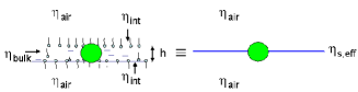
Figure 2: Schematic of the Trapeznikov approximation, where the entire soap film is approximated as a single interface in contact with bulk air phases. Reproduced with permission from Prasad and Weeks (2009).

The other consequence of the Trapeznikov approximation is that the hydrodynamics of a soap film must mimic that of a 2D fluid. To probe the hydrodynamics, we look at the correlated motions of particles embedded in the soap film. Similar to the treatment in Di Leonardo et al. (2008), we measure correlated and anti-correlated coupled displacements of particles to determine the ‘eigenmodes’ of particle motion in a 2D fluid. We give here a brief description of the method used by di Leonardo et al. Di Leonardo et al. (2008). They actively perturbed pairs of particles by means of optical tweezers in a soap film. The displacements of the particles from their mean particle positions are then determined. These displacements are related to strength of the trap and the mobility of the particles. The mobility of each particle is affected by the presence of the other particle, and therefore contains information about the nature of the flow fields in the soap film. The two dimensional Stokes equation can then be solved and the resulting motions of the particles decomposed into eigenmodes of motion. There are four such eigenmodes in 2D, given by $\lambda_{x\pm}$ and $\lambda_{y\pm}$ where $x$, $y$ represent motion parallel and perpendicular to the lines joining the centers of the particles and the $\pm$ represent rigid motions and relative displacements respectively. These mobilities are given by the equation

$$\lambda_{x\pm}=b[1\pm\frac{1}{4\pi\eta_{\text{bulk}}hb}\text{ln}(\frac{L}{R})]$$

$$\lambda_{y\pm}=b[1\pm\frac{1}{4\pi\eta_{\text{bulk}}hb}(\text{ln}(\frac{L}{R})-1)]$$ (5)

where $R$ is the separation between the particles, $L$ is a characteristic length scale and $b$ has units of mobility (kg^-1s). This length scale $L$ demands some explanation; flow fields in 2D are long-ranged and tend to diverge because of the presence of the logarithmic term in Eqn. III. This divergence is cut-off due to the presence of a length scale $L$, which has many possible origins. Some of these include finite size of the film, inertial effects, and viscous drag on the interfaces from the surrounding bulk fluid phases (air). In the subsequent sections, we will look at a series of soap films with different material parameters ($\eta_{\text{bulk}}$, $h$) and discuss in detail the origin of this length scale $L$. A detailed derivation of Eqn. III can also be found in reference Di Leonardo et al. (2008). It is clear from Eqn. III that the mobilities of the particles split around a mean mobility $b$, with rigid motions ($+$) being favored and relative displacements ($-$) being opposed. The hydrodynamic interactions between the particles are also governed by the fluid layer of the film, shown by the appearance of $\eta_{\text{bulk}}h$ in the equation.

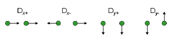
Figure 3: Coupled motions of particles embedded in the soap films. There are 4 possible eigenmodes associated with this coupling, correlated and anti-correlated motion parallel ($D_{x\pm}$) and perpendicular ($D_{y\pm}$) to the lines joining the centers of the particles.

Our approach to determine the flow fields in soap films, while analogous to di Leonardo’s approach, has some important differences. We measure the correlated thermal motions of pairs of particles embedded in the soap films. There are four such eigenmodes in 2D, represented by $D_{x\pm}$ and $D_{y\pm}$ which correspond to the longitudinal and transverse components of coupled motion, with the $\pm$ representing correlated and anti-correlated motion respectively (refer Fig. 3). The correlation functions are given by Cui et al. (2004); Diamant et al. (2005)

$$D_{x\pm}(R,\tau)=\langle\frac{1}{2}[\Delta r_{x}^{i}(\tau)\pm\Delta r_{x}^{j}(\tau)]^{2}\delta(R-R^{ij})\rangle_{i\neq j}$$

$$D_{y\pm}(R,\tau)=\langle\frac{1}{2}[\Delta r_{y}^{i}(\tau)\pm\Delta r_{y}^{j}(\tau)]^{2}\delta(R-R^{ij})\rangle_{i\neq j}$$ (6)

where $i$, $j$ are particle indices, the subscripts $x$ and $y$ represent motion parallel and perpendicular to the line joining the centers of particles and $R^{ij}$ is the separation between particles $i$ and $j$. The average is performed over all possible pairs of particles with a given separation $R$. This has the advantage of averaging out correlations from other particles that are not part of the pair. We are therefore confident that many-body effects due to the presence of other particles are minimized in our correlation functions. Similar to Prasad et al. (2006), we observe that $D_{x\pm}$, $D_{y\pm}\sim\tau$ which enables the estimation of four $\tau$-independent quantities $\langle D_{x\pm}/\tau\rangle_{\tau}$ and $\langle D_{y\pm}/\tau\rangle_{\tau}$ depending only on $R$ and having units of a diffusion constant. In this manuscript, we shall discuss only these $\tau$-independent quantities.

These $\tau$-independent correlation functions have a physical interpretation; for instance, $\langle D_{x+}/2\tau\rangle_{\tau}$ is the diffusion constant of the center of mass of the particle pairs along the line joining their centers, while $\langle D_{x-}/2\tau\rangle_{\tau}$ is the diffusion constant of the interparticle separation. Our correlation functions can then be trivially related to di Leonardo’s eigenmobilities by the relation

$$\langle D_{x\pm}/\tau\rangle=2k_{B}T\lambda_{x\pm}$$

$$\langle D_{y\pm}/\tau\rangle=2k_{B}T\lambda_{y\pm}$$ (7)

From Eqn. III, we can then derive theoretical expressions for our thermally driven correlation functions which are given by

$$\langle D_{x\pm}/\tau\rangle=B[1\pm C\text{ln}(\frac{L}{R})]$$

$$\langle D_{y\pm}/\tau\rangle=B[1\pm C(\text{ln}(\frac{L}{R})-1)]$$ (8)

where $B=2k_{B}Tb$ has units of a diffusion constant and $C=1/(4\pi\eta_{\text{bulk}}hb)$ is a non-dimensional constant. In the subsequent section we explore the validity of these theoretical expressions for a range of soap films with varying $h/d$ and viscosity $\eta_{\text{bulk}}$ of the fluid layer comprising the soap films.

IV Flow fields in soap films

Particle motions in the soap films are quantified by measurements of the mean square displacement (MSD), $\langle\Delta r^{2}\rangle$, which is ensemble-averaged over all particles in the field of view. Figure 4 shows the MSD for one particular soap film (solid symbols, refer caption of figure for details) plotted against the lag time $\tau$. Also shown in the figure is the corresponding MSD for diffusion in a 3D solution that comprises the fluid layer of the soap film (open symbols). From the figure, it is clear that the MSD is linear with respect to $\tau$, indicating free diffusion. By comparing the two MSDs, it is also evident that diffusion in the soap film (solid circles) is faster than in the corresponding bulk solution (open circles). This makes sense, as the Trapeznikov approximation states that the particle is at an effective interface in contact with bulk air phases. Since the air phase has a significantly lower viscosity than the fluid layer, this speeds the diffusive motion of the particle. Finally, Eqn. 4 can be solved to estimate the effective surface viscosity $\eta_{S}$ from the slope of the MSD.

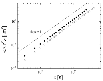
Figure 4: Mean square displacement (MSD) for a soap film, sample f in Table 1 (solid circles) compared to MSD in a bulk solution that comprises the fluid layer of the soap film (open circles). Dashed line shows a slope of 1, indicating free diffusion. The effective surface viscosity of the film can be evaluated from Eqn. 4, and is given by $\eta_{s,\text{eff}}=8.03$ nPa$\cdot$s.

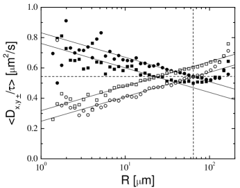
Figure 5: Correlation functions for the same soap film as in Fig. 4. Symbols are: $\langle D_{x+}/\tau\rangle$, solid circles; $\langle D_{x-}/\tau\rangle$, open circles; $\langle D_{y+}/\tau\rangle$, solid squares; $\langle D_{y-}/\tau\rangle$, open squares. Solid lines are fits to the data from Eqn III, with $B=0.54\mu$m²/s (horizontal dashed line), $C=0.13$ and $L=64\mu$m (vertical dashed line).

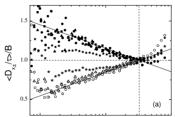
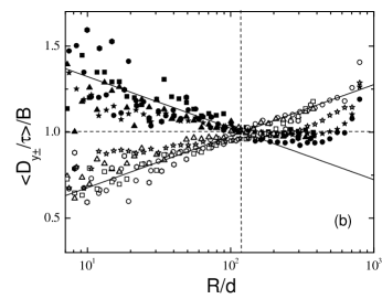
Figure 6: Scaled (a) longitudinal ($\langle D_{x\pm}/\tau\rangle/B$) and (b) transverse ($\langle D_{y\pm}/\tau\rangle/B$) correlation functions for five soap films plotted against the scaled separation $R/d$. Solid symbols represent correlated motion while open symbols represent anti-correlated motion. Refer Table 1 for details about the soap films. Symbols are: triangles, sample a; hexagons, sample c; squares, sample d; circles, sample f; stars, sample i. Solid lines are fits of the form $1\pm 0.13~{}\text{ln}(325d/R)$ and $1\pm 0.13(\text{ln}(325d/R)-1)$ respectively.

After the effective surface viscosity has been determined, we attempt to determine the flow fields in this soap film. This is done by looking at the correlated and anti-correlated motions of pairs of particles, as described in Sec. II.2 of this manuscript. The four correlation functions $\langle D_{x+}/\tau\rangle$, $\langle D_{x-}/\tau\rangle$, $\langle D_{y+}/\tau\rangle$ and $\langle D_{y-}/\tau\rangle$ are shown in Fig. 5 as a function of particle separation $R$. From the figure, it is clear that the correlation functions split around a mean diffusion constant $B$, with rigid motions (+, solid symbols) being favored and relative motions (-, open symbols) opposed. Further, the correlation functions vary logarithmically as a function of $R$, evidenced by the linearity of the data on a log-lin plot. In fact, the data are well characterized by Eqn. III, where $B$, $C$ and $L$ are fitting parameters. A visual way of determining the fit parameters is by noting that $\langle D_{x+}/\tau\rangle=\langle D_{x-}/\tau\rangle=B$ when $R=L$. Therefore, the dashed horizontal and vertical lines in the figure indicate that $B=0.54\mu$m²/s and $L=64\mu$m, while the slope of the four correlations functions simply gives $C=0.13$. These values have been used to fit the four correlation functions with Eqn. III in Fig. 5. We should note that the length scale determined above is smaller than the field of view of the microscope, and is therefore not subject to finite size effects; that is, it truly represents a cut-off length scale for stresses in this particular soap film. Further, as $B$ has units of a diffusion constant, it can be related to the self-diffusion of a single particle in the soap film (by replacing $R=d$ in Eqn. III). Finally, the constant $C=0.13$ represents how quickly the flow fields decay in this particular soap film.

Table 1: Material parameters for the nine soap films described in this paper. $\eta_{\text{{bulk}}}$ (determined from diffusivity measurements in bulk solutions) has an error of $\pm 5\%$, and values of $h$ and $d$ are certain to within $\pm 2\%$. The uncertainties in $\eta_{\text{int}}$, derived from Eqn. 1 and 2, are given in the brackets.

$\eta_{\text{bulk}}$ [mPa$\cdot$s]	$h$ [nm]	$d$ [nm]	$h/d$
a. 2.3	305	500	0.6
b. 3.0	640	500	1.3
c. 6.0	510	500	1.0
d. 10.0	1340	500	2.7
e. 25.0	1100	500	2.2
f. 10.0	780	210	3.7
g. 25.0	2184	210	10.4
h. 30.0	2100	210	10.0
i. 30.0	3000	210	14.3

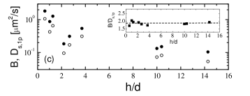
Figure 7: Fit parameters for nine soap films, including the five shown in Fig. 6, as a function of $h/d$. (a) $C$; the dashed line indicates a constant value of 0.13 for all soap films with $h/d<7\pm 3$. (b) $L/d$; the dashed line represents a value of 325, from the scaling of the correlation functions shown in Fig. 6. (c) $B$ (solid circles) compared to the one-particle diffusion constant $D_{s,1p}$ (open circles). The inset shows the ratio $B/D_{s,1p}$ to be nearly constant with a value of 1.9 $\pm$ 0.1.

To test the validity of the functional form of the correlation functions, we measure and plot their values for different soap films with a range of bulk viscosities, thickness and tracer particle sizes. This is shown in Figs. 6(a) and (b), where we have non-dimensionalized the correlation functions by the scale factor $B$ and the separation $R$ by the particle diameter $d$ for five different soap films, including the one shown in Fig. 5. We find that for all soap films with $h/d<7$, the longitudinal correlation functions scale onto a single curve, that is described by the equation $1\pm 0.13~{}\text{ln}(325d/R)$. For the film where $h/d=14.3$ (stars), there is significant deviation from the scaling, particularly relating to the slope $C$ ($C=0.06$ instead of 0.13). Similarly, the transverse correlation functions for the thin films can be well described by the form $1\pm 0.13~{}(\text{ln}(325d/R)-1)$, while the thicker films again deviate from the scaling (the transverse correlation functions are noisier than their longitudinal counterparts, hence the deviation is not as clearly visible). The dashed horizontal lines in Fig. 6(a) and (b) depict the splitting of the normalized diffusion constants around a value of 1, while the vertical lines are placed at values of $R/d=325$ and $325/e~{}(=120)$ for the longitudinal and transverse correlation functions respectively.

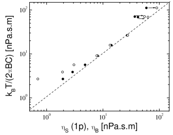
Figure 8: The scaled fit parameter $k_{B}T/(2\pi BC)$ compared to the one-particle effective surface viscosity $\eta_{S}$ (solid circles) and $\eta_{B}$ (open circles). The dashed line indicates equality between the two quantities.

The fitting parameters from the five soap films described above, as well as four additional ones are shown in Fig. 7. The fit parameter $C$ is plotted against $h/d$ in Fig. 7(a), where we see that $C\approx 0.13$ for all films with $h/d<7\pm 3$, while $C\approx 0.06$ for thicker films. On the other hand, the parameter $L/d$ shown in Fig. 7(b) is nearly constant for all soap films. Finally, in Fig. 7(c) we plot both $B$ and $D_{s,1p}$ as a function of $h/d$. Neither the fit parameter nor the one-particle diffusion constant show any discernible trend with $h/d$; however, judging by their equidistant separation on a logarithmic scale, they seem to be correlated together in some fashion. Indeed, plotting $B/D_{s,1p}$ against $h/d$, we find that $B/D_{s,1p}\approx 1.9\pm 0.1$ for all soap films. This is perhaps surprising, as $D_{s,1p}$ is a local measurement determined from the trajectory of single particles, while $B$ is obtained from the correlated motion of pairs of particles.

These parameters can be understood by considering various potentially relevant quantities which all have units of surface viscosity. The first quantity is $\eta_{B}=\eta_{\text{bulk}}h$. This product shows up in the theory (Eqns. III, III and III), and is an appealing quantity because it depends on two physical parameters that are easy to measure. The second quantity is the effective surface viscosity $\eta_{S}$ as determined from the one-particle measurements (Eqn. 4). The third quantity comes from the Trapeznikov approximation (Eqn. 3), which states that the entire soap film can be considered as an effective interface with a larger surface viscosity $\eta_{T}=\eta_{\text{bulk}}h+2\eta_{\text{int}}=\eta_{B}+2\eta_{\text{int}}$, thus suggesting that $\eta_{T}$ is more relevant than the first quantity $\eta_{B}$. The fourth quantity is the combination $k_{B}T/(2\pi BC)$, based on the two-particle correlations. From examining the theoretical expressions for the correlation functions described in Eqns. III, III and III, we see that $B=2k_{B}Tb$ and $C=1/(4\pi\eta_{\text{bulk}}hb)$, so that $k_{B}T/(2\pi BC)=\eta_{B}$. Thus, testing this equality is a test of that theory. In particular, the contribution to $\eta_{T}$ from $\eta_{\text{int}}$ has not been included in the expression for $C$, and so it is possible that the theory needs to be modified. We note that the fluid layer in the soap film studied by di Leonardo et al. Di Leonardo et al. (2008) consisted primarily of glycerol, and presumably $\eta_{\text{int}}$ was irrelevant for their system, that is, $\eta_{B}\approx\eta_{T}\gg\eta_{\text{int}}$. This is not true for our soap films, as we have situations where $\eta_{B}\sim\eta_{\text{int}}$ as well as $\eta_{B}\gg\eta_{\text{int}}$.

To test these conjectures, we compare these three quantities in Fig. 8, where we plot the scaled quantity $k_{B}T/(2\pi BC)$ against the measured one-particle effective surface viscosity $\eta_{S}$ (solid circles) and $\eta_{B}$ (open circles). For thin films with low surface viscosities (lower left corner of the graph), we see the solid symbols for $\eta_{S}$ are to the right of the open symbols for $\eta_{B}$, in agreement with the Trapeznikov approximation. From the difference in these two quantities, one can extract the surface viscosity $\eta_{\text{int}}$ which we have done previously for these data, finding $\eta_{\text{int}}=0.97\pm 0.55$ nPa$\cdot$s$\cdot$m Prasad and Weeks (2009). However, for thicker films with higher surface viscosities (top right corner of Fig. 8), we see the opposite is true; the effective surface viscosities $\eta_{S}$ (solid circles) are lower than $\eta_{B}$ (open circles), showing that Saffman’s equation (Eqn. 4) measures a viscosity that is too low. This occurs even though the thick films still behave as a 2D fluid according to their correlation functions, in other words, Eqns. III, III and III still describe the two-particle correlations, albeit with different parameters.

The comparison with $k_{B}T/(2\pi BC)$ in Fig. 8 bolsters these conclusions. For thin films, $\eta_{S}$ matches better with $k_{B}T/(2\pi BC)$ (comparison of solid symbols with the dashed line, lower left of Fig. 8). For thicker films, $\eta_{B}$ matches better (comparison of open symbols with the dashed line, upper right of Fig. 8). Our data suggest that in the theory leading to Eqns. III, III, and III, we should replace $\eta_{B}=\eta_{\text{bulk}}h$ with $\eta_{T}$; this minor correction would improve the results for thin, less viscous films, and be negligible for thicker viscous films such as those studied in Ref. Di Leonardo et al. (2008). The disagreement between $k_{B}T/(2\pi BC)$ and $\eta_{S}$ shows the breakdown of the applicability of Saffman’s equation to extract a useful surface viscosity from one-particle data, for situations with $h/d>7$, and in fact coincides with a breakdown of the equality $\eta_{S}=\eta_{T}$ Prasad and Weeks (2009).

To summarize, for all films we have $k_{B}T/(2\pi BC)=\eta_{T}$ and for thin films we additionally have $\eta_{S}=\eta_{T}$. The approximation $\eta_{B}\approx\eta_{T}$ is mathematically obvious for thick films, given the definitions of these two surface viscosities. It is worth noting that our prior work suggests that it is necessary to measure $\eta_{S}$ (in thin films) to be able to determine $\eta_{T}$, as the viscosity of the surfactant layers $\eta_{\text{int}}$ is usually not known ahead of time Prasad and Weeks (2009); this current work suggests that measuring $k_{B}T/(2\pi BC)$ is an additional method to obtain $\eta_{T}$ and thus $\eta_{\text{int}}$.

Using these insights, we return to the data shown in Fig. 7. For low values of $h/d$, $C$ is constant, as shown in panel (a); meanwhile, $B$ drops, as shown in panel (c). This suggests that the mobility $b$ scales as $b\sim\eta_{T}^{-1}$ for thin films. Indeed, this explains the correlations of $B$ and $D_{s,1p}$ seen in Fig. 7(c) for thin films, as $D_{s,1p}\sim 1/\eta_{T}$ would be expected Prasad and Weeks (2009). However, at thicker films, $C$ decreases, suggesting that $b$ grows faster than $\eta_{T}^{-1}$; the mobility of particles increases. This is consistent with Saffman’s equation incorrectly yielding a surface viscosity $\eta_{S}$ that is too low for the thicker films.

We also note that the parameter $L/d$ is nearly constant for all soap films. This is very surprising, as the logarithmic cut-off in the decay of the correlation functions can arise from three possible factors: 1) finite size of the film; (2) inertial effects; and (3) viscous drag on the soap film from the bulk air phases. The size of the frame used to house the film is of order $\sim$ 1 cm, which is too large to explain the values of $L$ obtained from fits to the correlation functions. Inertial effects arise at length scales given by $L=\eta_{\text{bulk}}/\rho U$, where $\rho$ is the fluid density and $U$ is a typical probe particle speed. This gives length scales of order $\sim$ 1m, which is again too large to explain our fit-derived length scales. Finally, the viscous cut-off length scale is given by $L=\eta_{s,\text{eff}}/\eta_{\text{air}}$. Clearly, as can be seen from Fig. 8, this length scale must increase as the effective surface viscosity increases. Therefore, the near-constant value of $L/d$ for soap films over a range of $\eta_{s,\text{eff}}$ remains a mystery. Note that none of these potential origins for $L$ would predict any dependence on the particle size $d$; that is, they might predict a film-independent $L$ but not a constant $L/d$ as we find (from data including two different particle sizes $d$ differing by a factor of 2.4).

One additional particle-based explanation for the constant value of $L/d$ could be capillary effects. Capillary effects arise from deformation of the interface by the particle, with an energy gain obtained when two particles stick to each other. However, it isn’t obvious that this moderately short range interaction would lead to such a very long length scale as we observe ($L/d\sim 325$). We leave the reasons for the constant value of $L/d$ as a matter for future research.

V Conclusion

We have used the technique of two-particle microrheology to characterize the flow fields in soap films of varying thickness $h$, where $0.6\leq h/d\leq 14.3$ (based on probe diameter $d$). In particular, we determine the ‘eigenmobilities’ of thermally correlated motions of probe particles in these soap films. These eigenmobilities consist of correlated motion parallel and perpendicular to the lines joining the centers of pairs of particles, and rigid and relative motion as well. The eigenmobilities are found to split around a mean value and decay logarithmically as a function of particle separation for all soap films. The flow fields of all films we observe are well described by theoretical models. A study of the fit parameters shows that thin films have a simple behavior, where a surface viscosity $\eta_{T}$ predicted by Trapeznikov over 50 years ago correctly describes both one-particle and two-particle motions Trapeznikov (1957). In fact, for the thinnest films, our results suggest that prior theoretical work should be modified slightly to use $\eta_{T}$ Di Leonardo et al. (2008). In our work we also a transition from ‘pure-2D’ to ‘3D-influenced’ behavior at $h/d=7\pm 3$. For thicker films, two-particle correlations still follow the predicted form for a quasi-2D fluid, with surface viscosity $\eta_{T}$. However, one-particle motion is faster than expected, and other significant deviations from the thin-film behavior are noted. The results of our study on soap films can have important consequences for other 2D systems, including but not limited to microfluidic flow in confined geometries, protein and surfactant monolayers at an air water interface and the cell membrane.

Funding for this work was provided by the National Science Foundation (DMR-0804174) and the Petroleum Research Fund, administered by the American Chemical Society (47970-AC9). We thank J. Gallivan for use of the spectrophotometer, and H. Diamant, H. A. Stone, and E. van Nierop for helpful discussions.

References

- Stone and Ajdari (1998) H. A. Stone and A. Ajdari, J. Fluid. Mech. 369, 151 (1998).
- Levine and MacKintosh (2002) A. J. Levine and F. C. MacKintosh, Phys. Rev. E. 66, 061606 (2002).
- Fischer (2004) T. M. Fischer, J. Fluid. Mech. 498, 123 (2004).
- Di Leonardo et al. (2008) R. Di Leonardo, S. Keen, F. Ianni, J. Leach, M. J. Padgett, and G. Ruocco, Phys. Rev. E 78, 031406 (2008).
- Cheung et al. (1996) C. Cheung, Y. H. Hwang, X. L. Wu, and H. J. Choi, Phys. Rev. Lett. 76, 2531 (1996).
- Mathé et al. (2008) J. Mathé, J. M. Di Meglio, and B. Tinland, J. Colloid Interfac. Sci. 322, 315 (2008).
- Martin and Wu (1995) B. Martin and X. I. Wu, Rev. Sci. Instrum. 66, 5603 (1995).
- Vorobieff and Ecke (1999) P. Vorobieff and R. E. Ecke, Phys. Rev. E 60, 2953 (1999).
- Crocker et al. (2000) J. C. Crocker, M. T. Valentine, E. R. Weeks, T. Gisler, P. D. Kaplan, A. G. Yodh, and D. A. Weitz, Phys. Rev. Lett. 85, 888 (2000).
- Levine and Lubensky (2000) A. J. Levine and T. C. Lubensky, Phys. Rev. Lett. 85, 1774 (2000).
- Gardel et al. (2003) M. L. Gardel, M. T. Valentine, J. C. Crocker, A. R. Bausch, and D. A. Weitz, Phys. Rev. Lett. 91 (2003), 158302.
- Starrs and Bartlett (2003) L. Starrs and P. Bartlett, J. Phys: Cond. Matt. 15, 251 (2003).
- Dasgupta and Weitz (2005) B. R. Dasgupta and D. A. Weitz, Phys. Rev. E. 71 (2005), 021504.
- Lau et al. (2003) A. W. C. Lau, B. D. Hoffman, A. Davies, J. C. Crocker, and T. C. Lubensky, Phys. Rev. Lett. 91, 198101 (2003).
- Prasad et al. (2006) V. Prasad, S. A. Koehler, and E. R. Weeks, Phys. Rev. Lett. 97, 176001 (2006).
- Prasad and Weeks (2009) V. Prasad and E. R. Weeks, Phys. Rev. Lett. 102, 178302 (2009).
- Trapeznikov (1957) A. A. Trapeznikov, Proceedings of the 2nd International Congress on Surface Activity (1957).
- Crocker and Grier (1996) J. C. Crocker and D. G. Grier, J. Colloid Interfac. Sci. 179, 298 (1996).
- Mason et al. (1997) T. G. Mason, A. Dhople, and D. Wirtz, Mat.Res. Soc. Symp. Proc. 463, 153 (1997).
- Huibers and Shah (1997) P. D. T. Huibers and D. O. Shah, Langmuir 13, 5995 (1997).
- Saffman and Delbrück (1975) P. G. Saffman and M. Delbrück, Proc. Natl. Acad. Sci. USA 72, 3111 (1975).
- Cui et al. (2004) B. X. Cui, H. Diamant, B. H. Lin, and S. A. Rice, Phys. Rev. Lett. 92, 258301 (2004).
- Diamant et al. (2005) H. Diamant, B. Cui, B. Lin, and H. Diamant, J. Physics: Cond. Matt. 17, 2787 (2005).