NUMERICAL ASPECTS OF EVOLUTION OF PLANE CURVES SATISFYING THE FOURTH ORDER GEOMETRIC EQUATION

Abstract

In this review paper we present a stable Lagrangian numerical method for computing plane curves evolution driven by the fourth order geometric equation. The numerical scheme and computational examples are presented.

1 Introduction

The main purpose of this contribution is to suggest a method for computing evolution of closed smooth plane curves driven by the normal velocity $\beta$ depending on the intrinsic Laplacian of the curvature $k$ and curvature itself:

$$\beta=-\partial^{2}_{s}k+b(k)$$ (1)

where $b(k)$ is a $C^{2}$ function of the curvature $k$, $b(0)=0$. Numerical aspects of evolution of plane curves satisfying (1) have been studied in [1] for the case of the surface diffusion flow with no lower order terms, i.e. $\beta=-\partial^{2}_{s}k$, and in [2] for the case of the so-called Willmore flow for which the normal velocity is given by $\beta=-\partial^{2}_{s}k-\frac{1}{2}k^{3}$. Recall that the latter case corresponds to the motion of elastic curves, e.g. the model of Euler-Bernoulli elastic rod, which is an important problem in structural mechanics. The elastic curve evolution and surface diffusion can be found in many practical applications as sintering (in brick production), formation of rock strata from sandy sediments, metal thin film growth etc. (see e.g. [3]).

2 Governing equations

We follow the so-called direct (or Lagrangian) approach. We represent a solution of (1) by the position vector $x$ satisfying the geometric equation $\partial_{t}x=\beta\vec{N}+\alpha\vec{T}$ where $\vec{N},\vec{T}$ are the unit inward normal and tangent vectors. An immersed regular plane curve $\Gamma$ can be parameterized by a smooth function $x:S^{1}\to\mathbb{R}^{2}$, i.e. $\Gamma=\{x(u),u\in S^{1}\}$, for which $g=|\partial_{u}x|>0$. Taking into account the periodic boundary conditions at $u=0,1$ we shall hereafter identify $S^{1}$ with the interval $[0,1]$. The unit arc-length parameterization will be denoted by $s$, so $\mbox{d}s=g\,\mbox{d}u$. The tangent vector $\vec{T}$ and the signed curvature $k$ of $\Gamma$ satisfy $\vec{T}=\partial_{s}x$, $k=\mbox{det}(\partial_{s}x,\partial^{2}_{s}x)$. Moreover, we choose the unit inward normal vector $\vec{N}$ such that $\mbox{det}(\vec{T},\vec{N})=1$. Let a regular smooth initial curve $\Gamma_{0}=\mathop{\mathrm{missing}}{Image}(x_{0})$ be given. It turns out that a family of plane curves $\Gamma_{t}=\mathop{\mathrm{missing}}{Image}(x(.,t)),t\in[0,T)$, satisfying (1) can be represented by a solution to the following system of PDEs:

$$\partial_{t}k=-\partial^{4}_{s}k+\partial^{2}_{s}b(k)+\partial_{s}(\alpha k)+k(k\beta-\partial_{s}\alpha),$$ (2)

$$\partial_{t}\eta=-k\beta+\partial_{s}\alpha,\ \ \ g=\exp(\eta),$$ (3)

$$\partial_{t}x=-\partial_{s}^{4}x-\frac{k^{3}-b(k)}{k}\partial^{2}_{s}x+(\alpha-\frac{3}{2}\partial_{s}(k^{2}))\partial_{s}x\,,$$ (4)

subject to initial conditions $k(.,0)=k_{0}\,,\ g(.,0)=g_{0}\,,\ x(.,0)=x_{0}(.)$ and periodic boundary conditions at $u=0,1$ (cf. [4, 5]).

3 Approximation scheme and numerical experiments

The presence of a tangential velocity $\alpha$ in the position vector equation has no impact on the shape of evolving curves. As it was shown e.g. in [6, 7, 8, 9, 4, 5] for general curvature driven motions (nonlinear, anisotropic, with external forces) incorporation of a suitable tangential velocity into governing equations stabilizes numerical computations significantly. It prevents the direct Lagrangian algorithm from its main drawbacks – the merging of numerical grid points and their order exchange. It also allows for larger time steps without loosing stability. In our numerical solution we consider tangential velocity given by a nonlocal tangential redistributions discussed in a detail in [8, 9, 4, 5]. It follows from [4, 5] that the redistribution functional $\alpha$ satisfying

$$\partial_{s}\alpha=k\beta-\langle k\beta\rangle_{\Gamma}+\omega\left(L/g-1\right)\,,$$ (5)

with a constant $\omega>0$, is capable of asymptotic uniform redistribution of grid points along the evolved curve. In our computational method a numerically evolved curve is represented by discrete plane points $x_{i}^{j}$ where the index $i=1,...,n,$ denotes space discretization and the index $j=0,...,m,$ denotes a discrete time stepping. The linear approximation of an evolving curve in the $j$-th discrete time step is thus given by a polygon with vertices $x_{i}^{j},i=1,...,n$. Due to periodicity conditions we shall also use additional values $x_{-1}^{j}=x_{n-1}^{j}$, $x_{0}^{j}=x_{n}^{j}$, $x_{n+1}^{j}=x_{1}^{j}$, $x_{n+2}^{j}=x_{2}^{j}$. If we take a uniform division of the time interval $[0,T]$ with a time step $\tau=\frac{T}{m}$ and a uniform division of the fixed parameterization interval $[0,1]$ with a step $h=\frac{1}{n}$, a point $x_{i}^{j}$ corresponds to $x(ih,j\tau)$. The systems of difference equations corresponding to (2)–(4) and (5) will be given for discrete quantities $\alpha_{i}^{j}$, $\eta_{i}^{j}$, $r_{i}^{j}$, $k_{i}^{j}$, $x_{i}^{j}$, $i=1,...,n,\ j=1,...,m$, representing approximations of the unknowns $\alpha$, $\eta$, $gh$, $k$, and $x$, respectively. Here $\alpha_{i}^{j}$ represents tangential velocity of a flowing node $x_{i}^{j}$, and $\eta_{i}^{j}$, $r_{i}^{j}\approx|x_{i}^{j}-x_{i-1}^{j}|$, $k_{i}^{j}$, $\nu_{i}^{j}$ represent piecewise constant approximations of the corresponding quantities in the so-called flowing finite volume $\left[x_{i-1}^{j},x_{i}^{j}\right]$. We shall use the corresponding flowing dual volumes $\left[\tilde{x}_{i-1}^{j},\tilde{x}_{i}^{j}\right]$, where $\tilde{x}_{i}^{j}=\frac{x_{i-1}^{j}+x_{i}^{j}}{2}$, with approximate lengths $q_{i}^{j}\approx|\tilde{x}_{i}^{j}-\tilde{x}_{i-1}^{j}|$. At the $j$-th discrete time step, we first find discrete values of the tangential velocity $\alpha_{i}^{j}$ by discretizing equation (5). Then the values of redistribution parameter $\eta_{i}^{j}$ are computed and utilized for updating discrete local lengths $r_{i}^{j}$ by discretizing equations (3). Using already computed local lengths, the intrinsic derivatives are approximated in (2), and (4), and pentadiagonal systems with periodic boundary conditions are constructed and solved for discrete curvatures $k_{i}^{j}$ and position vectors $x_{i}^{j}$. In the sequel, we present in a more detail our discretization. Using $r_{i}^{j-1}$ as an approximation of the length of the flowing finite volume $\left[x_{i-1}^{j-1},x_{i}^{j-1}\right]$ at the previous $j$th time step we construct difference approximation of the intrinsic derivative $\partial_{s}\alpha\approx\frac{\alpha_{i}^{j}-\alpha_{i-1}^{j}}{r_{i}^{j-1}}$ and by taking all further quantities in (5) from the previous time step. We obtain the following expression for discrete values of the tangential velocity: $\alpha_{i}^{j}=\alpha_{i-1}^{j}+r_{i}^{j-1}k_{i}^{j-1}\beta_{i}^{j-1}-r_{i}^{j-1}B^{j-1}+\omega(M^{j-1}-r_{i}^{j-1})$ where $\beta_{i}^{j-1}=-\frac{1}{r_{i}^{j-1}}\left(\frac{k_{i+1}^{j-1}-k_{i}^{j-1}}{q_{i}^{j-1}}-\frac{k_{i}^{j-1}-k_{i-1}^{j-1}}{q_{i-1}^{j-1}}\right)+b(k_{i}^{j-1})$, $q_{i}^{j-1}=\frac{r_{i}^{j-1}+r_{i+1}^{j-1}}{2}$, $M^{j-1}=\frac{1}{n}L^{j-1}$, $L^{j-1}=\sum\limits_{l=1}^{n}r_{l}^{j-1}$, $B^{j-1}=\frac{1}{L^{j-1}}\sum\limits_{l=1}^{n}r_{l}^{j-1}k_{l}^{j-1}\beta_{l}^{j-1}$ and $\alpha_{0}^{j}=0$, i.e. the point $x_{0}^{j}$ is moved in the normal direction only. Inserting (5) in (3) and using a similar strategy give us: $r_{i}^{j-1}\frac{\eta_{i}^{j}-\eta_{i}^{j-1}}{\tau}=-r_{i}^{j-1}B^{j-1}+\omega(M^{j-1}-r_{i}^{j-1})$, for $i=1,...,n,\eta_{0}^{j}=\eta_{n}^{j},\ \ \eta_{n+1}^{j}=\eta_{1}^{j}$. Next we update local lengths by the rule: $r_{i}^{j}=\exp(\eta_{i}^{j}),r_{-1}^{j}=r_{n-1}^{j},\ \ r_{0}^{j}=r_{n}^{j},\ \ r_{n+1}^{j}=r_{1}^{j},\ \ r_{n+2}^{j}=r_{2}^{j}.$ Subsequently, new local lengths are used for approximation of intrinsic derivatives in (2) and (4). First, we derive a discrete analogy of the curvature equation (2). We have to approximate the 4-th order derivative of curvature inside the flowing finite volume $\left[x_{i-1},x_{i}\right]$, $i=1,...,n$. For that goal we take the following finite difference approximation: $\partial_{s}^{4}k(\tilde{x}_{i})\approx\frac{1}{r_{i}q_{i}r_{i+1}q_{i+1}}k_{i+2}-\bigl{(}\frac{1}{r_{i}q_{i}r_{i+1}q_{i+1}}+\frac{1}{r_{i}q_{i}^{2}r_{i+1}}+\frac{1}{r_{i}^{2}q_{i}^{2}}+\frac{1}{r_{i}^{2}q_{i}q_{i-1}}\bigr{)}k_{i+1}+\bigl{(}\frac{1}{r_{i}q_{i}^{2}r_{i+1}}+\frac{1}{r_{i}^{2}q_{i}^{2}}+\frac{2}{r_{i}^{2}q_{i}q_{i-1}}+\frac{1}{r_{i}^{2}q_{i-1}^{2}}+\frac{1}{r_{i}q_{i-1}^{2}r_{i-1}}\bigr{)}k_{i}+\bigl{(}\frac{1}{r_{i}^{2}q_{i}q_{i-1}}+\frac{1}{r_{i}^{2}q_{i-1}^{2}}+\frac{1}{r_{i}q_{i-1}^{2}r_{i-1}}+\frac{1}{r_{i}q_{i-1}r_{i-1}q_{i-2}}\bigr{)}k_{i-1}+\frac{1}{r_{i}q_{i-1}r_{i-1}q_{i-2}}k_{i-2}$. Approximating first and second order terms in (2) by central differences and taking semi-implicit time stepping we obtain following pentadiagonal system with periodic boundary conditions for new discrete values of curvature:

$$a_{i}^{j}k_{i-2}^{j}+b_{i}^{j}k_{i-1}^{j}+c_{i}^{j}k_{i}^{j}+d_{i}^{j}k_{i+1}^{j}+e_{i}^{j}k_{i+2}^{j}=f_{i}^{j}$$

subject to periodic b.c. $k_{-1}^{j}=k_{n-1}^{j},k_{0}^{j}=k_{n}^{j},k_{n+1}^{j}=k_{1}^{j},k_{n+2}^{j}=k_{2}^{j},$ where

$$a_{i}^{j}=\frac{1}{q_{i-1}^{j}r_{i-1}^{j}q_{i-2}^{j}},\ \ e_{i}^{j}=\frac{1}{q_{i}^{j}r_{i+1}^{j}q_{i+1}^{j}},$$

$$f_{i}^{j}=\frac{r_{i}^{j}}{\tau}k_{i}^{j-1}+\frac{b(k_{i+1}^{j-1})-b(k_{i}^{j-1})}{q_{i}^{j}}-\frac{b(k_{i}^{j-1})-b(k_{i-1}^{j-1})}{q_{i-1}^{j}},$$

$$b_{i}^{j}=-\left(\frac{1}{r_{i}^{j}q_{i}^{j}q_{i-1}^{j}}+\frac{1}{r_{i}^{j}(q_{i-1}^{j})^{2}}+\frac{1}{(q_{i-1}^{j})^{2}r_{i-1}^{j}}+\frac{1}{q_{i-1}^{j}r_{i-1}^{j}q_{i-2}^{j}}\right)+\frac{\alpha_{i-1}^{j}}{2}$$

$$d_{i}^{j}=-\left(\frac{1}{q_{i}^{j}r_{i+1}^{j}q_{i+1}^{j}}+\frac{1}{(q_{i}^{j})^{2}r_{i+1}^{j}}+\frac{1}{r_{i}^{j}(q_{i}^{j})^{2}}+\frac{1}{r_{i}^{j}q_{i}^{j}q_{i-1}^{j}}\right)-\frac{\alpha_{i}^{j}}{2}$$

$$c_{i}^{j}=\frac{1}{(q_{i}^{j})^{2}r_{i+1}^{j}}+\frac{1}{r_{i}^{j}(q_{i}^{j})^{2}}+\frac{2}{r_{i}^{j}q_{i}^{j}q_{i-1}^{j}}+\frac{1}{r_{i}^{j}(q_{i-1}^{j})^{2}}+\frac{1}{(q_{i-1}^{j})^{2}r_{i-1}^{j}}+$$

$$\hskip 28.45274pt\frac{r_{i}^{j}}{\tau}-r_{i}^{j-1}k_{i}^{j-1}\beta_{i}^{j-1}+\frac{\alpha_{i}^{j}}{2}-\frac{\alpha_{i-1}^{j}}{2}.$$

In order to construct discretization of equation (4) we approximate the intrinsic derivatives in a dual volume $\left[\tilde{x}_{i-1},\tilde{x}_{i}\right]$. For approximation of the fourth order intrinsic derivative of the position vector we take similar approach as above for curvature, but in the middle point $x_{i}$ of the dual volume. In such a way and using the semi-implicit approach, we end up with two tridiagonal systems for updating the discrete position vector:

$${\cal A}_{i}^{j}x_{i-2}^{j}+{\cal B}_{i}^{j}x_{i-1}^{j}+{\cal C}_{i}^{j}x_{i}^{j}+{\cal D}_{i}^{j}x_{i+1}^{j}+{\cal E}_{i}^{j}x_{i+2}^{j}={\cal F}_{i}^{j}\$$

for $i=1,...,n\,$ subject to periodic b.c. $x_{-1}^{j}=x_{n-1}^{j},\ \ x_{0}^{j}=x_{n}^{j},\ \ x_{n+1}^{j}=x_{1}^{j},\ \ x_{n+2}^{j}=x_{2}^{j}$ where

$${\cal A}_{i}^{j}=\frac{1}{r_{i}^{j}q_{i-1}^{j}r_{i-1}^{j}},\ {\cal E}_{i}^{j}=\frac{1}{r_{i+1}^{j}q_{i+1}^{j}r_{i+2}^{j}},\$$

$${\cal B}_{i}^{j}=-\left(\frac{1}{r_{i}^{j}q_{i-1}^{j}r_{i-1}^{j}}+\frac{1}{(r_{i}^{j})^{2}q_{i-1}^{j}}+\frac{1}{(r_{i}^{j})^{2}q_{i}^{j}}+\frac{1}{r_{i}^{j}q_{i}^{j}r_{i+1}^{j}}\right)+$$

$$\hskip 28.45274pt+\ \frac{\phi(k_{i}^{j})+\phi(k_{i-1}^{j})}{2r_{i}^{j}}+\frac{\alpha_{i}^{j}}{2}-\frac{3}{4}\frac{(k_{i+1}^{j})^{2}-(k_{i}^{j})^{2}}{q_{i}^{j}}$$

$${\cal D}_{i}^{j}=-\left(\frac{1}{r_{i}^{j}q_{i}^{j}r_{i+1}^{j}}+\frac{1}{(r_{i+1}^{j})^{2}q_{i}^{j}}+\frac{1}{(r_{i+1}^{j})^{2}q_{i+1}^{j}}+\frac{1}{r_{i+1}^{j}q_{i+1}^{j}r_{i+2}^{j}}\right)+$$

$$\hskip 28.45274pt+\ \frac{\phi(k_{i+1}^{j})+\phi(k_{i}^{j})}{2r_{i+1}^{j}}-\frac{\alpha_{i}^{j}}{2}+\frac{3}{4}\frac{(k_{i+1}^{j})^{2}-(k_{i}^{j})^{2}}{q_{i}^{j}}\,,$$

$${\cal C}_{i}^{j}=\frac{q_{i}^{j}}{\tau}-({\cal A}_{i}^{j}+{\cal B}_{i}^{j}+{\cal D}_{i}^{j}+{\cal E}_{i}^{j}),\ {\cal F}_{i}^{j}=\frac{q_{i}^{j}}{\tau}x_{i}^{j-1},$$

where $\phi(k)=k^{2}-\frac{b(k)}{k}$. The initial quantities for the algorithm are computed from a discrete representation of the initial curve $x_{0}$, for details see [5]. Every pentadiagonal system is solved by mean of Gauss-Seidel iterations. Next we present results of numerical simulations for the curve evolution driven by (1). In our experiments evolving curves are represented by $n=100$ grid points and we use discrete time step $\tau=0.001$. First we numerically compute time evolution of the initial ellipse with the halfaxes ratio 2:1 for the case $b(k)=0$ (surface diffusion flow). We consider the time interval $[0,2]$. The evolution of curves without considering tangential redistribution indicates accumulation of some curve representing grid points and a poor resolution in other parts of the asymptotic shape, see also Figure 1, a). In the case of asymptotically uniform tangential redistribution, we can see a uniform discrete resolution of the asymptotic shape, see Figure 1, b). Next we present evolution of an nontrivial initial curve driven by (1) with $b(k)=0$. We show evolution of a highly nonconvex initial curve (see Figure 1, c) with asymptotically uniform redistribution ($\omega=1$). Since elastic curve dynamics is very fast in case of highly varying curvature along the curve we have chosen smaller time step $\tau=10^{-6}$. In Figure 2 we present evolution of an initial asteroid driven by (1) with $b(k)=-\frac{1}{2}k^{3}$ (the Willmore flow). A solution computed by the direct Lagrangian method is depicted by cross marks whereas solid curves correspond to the solution computed by the level set method approach. For details we refer the reader to [2].

       

a)                           b)                           c)

Figure 1: Surface diffusion of an initial ellipse and its circular asymptotic shapes without a) and with b) tangential redistribution. Evolution of the highly nonconvex initial curve and its asymptotic circular shape at time $t=0.170$ c).

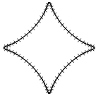
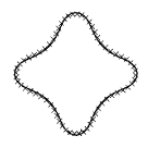
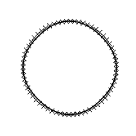
Figure 2: An asteroid as an initial condition and its evolution by the Willmore flow at times $t=0,\,0.0005,\,0.005$.

References

• [1] K. Mikula and D. Ševčovič, Proceedings of Algoritmy 2005, 17th Conference on Scientific Computing, Vysoke Tatry, Podbanske, Slovakia (2005).
• [2] M. Beneš, T. Mikula, K. Oberhuber and D. Ševčovič, Comp. and Vis. in Science, to appear (2008).
• [3] J. Sethian, Level set methods, Cambridge Monographs on Applied and Computational Mathematics, Vol. 3 (Cambridge University Press, Cambridge, 1996).
• [4] K. Mikula and D. Ševčovič, SIAM Journal on Applied Mathematics 61, 1473 (2001).
• [5] K. Mikula and D. Ševčovič, Comput. and Vis. in Science 6, 211 (2004).
• [6] K. Deckelnick, Calc. Var. Partial Differ. Equ. 5, 489 (1997).
• [7] G. Dziuk, Math. Models Methods Appl. Sci. 4, 589 (1994).
• [8] T. Y. Hou, J. S. Lowengrub and M. J. Shelley, J. Comput. Phys. 114, 312 (1994).
• [9] M. Kimura, Japan J. Indust. Appl. Math. 14, 373 (1997).