IFJPAN-IV-2009-2
Non-abelian infra-red cancellations in the unintegrated NLO kernel.

Abstract

Abstract: We investigate the infrared singularity structure of Feynman diagrams entering the next-to-leading-order (NLO) DGLAP kernel (non-singlet). We examine cancellations between diagrams for two gluon emission contributing to NLO kernels. We observe the crucial role of color coherence effects in cancellations of infra-red singularities. Numerical calculations are explained using analytical formulas for the singular contributions.

Submitted To Acta Physica Polonica B

12.38.-t, 12.38.Bx, 12.38.Cy

1 Introduction

This study is part of the effort with the aim of constructing fully-exclusive (unintegrated) kernels for DGLAP [1] evolution in QCD at the complete NLO level. More details on this project can be found in ref. [2]. Let us only mention that construction of the exclusive NLO DGLAP kernels in ref. [2] is done following Curci-Furmanski-Petronzio (CFP) scheme [3] and we adopt this scheme also in our study. In short the CFP scheme uses axial gauge and dimensional regularization ($\overline{MS}$) and generalizes collinear factorization developed in ref. [4]. The two particle-irreducible (2PI) evolution kernels $K_{0}$

$$M=C_{0}(1+K_{0}+K_{0}^{2}+...)=C_{0}\Gamma_{0}$$ (1)

are contracted with the coefficient functions $C_{0}$, which are infra-red finite. All infra-red collinear divergences are encapsulated in $\Gamma_{0}$, which denotes the sum over kernels $K_{0}$. The DGLAP NLO kernel is then extracted according to the scheme [3] as a single pole in $\Gamma_{0}$. More details can be found in ref. [3] and in ref. [2] of these proceedings.

As it is well known individual Feynman diagrams are not gauge-invariant and sizeable cancellations occur among them. In particular some graphs contributing to NLO DGLAP kernels may contain artificial infra-red singularities, which cancel in a bigger subset of diagrams and do not appear in the final results. Our aim is to analyze in detail such cancellations at the level of the exclusive distributions, before the phase space integration, for the diagrams contributing to NLO DGLAP kernels in the CFP scheme.

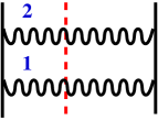
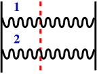
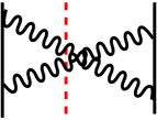
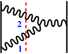
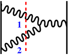
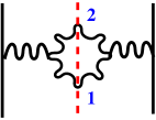
Figure 1: Two gluon Feynman diagrams contributing to non-singlet NLO kernels

We shall analyze singular infra-red structure of the Feynman diagrams depicted in Fig. 1. They describe emission of two gluons off a quark and enter into calculation of the non-singlet NLO kernel. Diagrams of Fig. 1-1 are bremsstrahlung type diagrams, including interference in Fig. 1. Their $C_{F}^{2}$ part is the same as in the corresponding case of QED, hence we shall sometimes call them “abelian”. The other diagrams of Fig. 1 include production of the gluon pair, see Fig. 1, and its interference with the previous bremsstrahlung diagrams, Figs. 1 and 1. Because of the presence of the triple-gluon vertex they are diagrams of the genuine non-abelian origin. Moreover, since the crossed-ladder diagram of Fig.1 carries color factor equal to $C_{F}^{2}-\frac{1}{2}C_{F}C_{A}$, it contributes to both “abelian” and “non-abelian” part of NLO kernel.

Let us now introduce notation. The two gluon phase-space is parametrized using Sudakov variables:

$$\begin{split}&k_{i}=\alpha_{i}p+\alpha_{i}^{-}n+k_{i\perp},\quad i=1,2,\\ &k=k_{1}+k_{2},\qquad q=p-k\end{split}$$ (2)

with $p$ being the four-momentum of the incoming quark and $n$ a light-cone vector. Four-vectors $k_{1}$ and $k_{2}$ denote four-momenta of the emitted gluons, with their transverse parts being $k_{1\perp}$ and $k_{2\perp}$ respectively, and $k^{2}=(k_{1}+k_{2})^{2}$ being their effective mass. The sum of $\alpha_{i}$ is fixed

$$\alpha_{1}+\alpha_{2}=1-x.$$ (3)

We shall examine the distributions of two gluons in the soft limit:

$$\begin{cases}\alpha_{1}\rightarrow 0\cr\alpha_{2}\rightarrow 1-x\end{cases}\text{ or }\begin{cases}\alpha_{1}\rightarrow 1-x\cr\alpha_{2}\rightarrow 0.\end{cases}$$ (4)

We shall also use the “eikonal minus variables” $v_{i}$ of the emitted gluons defined as

$$v_{i}=\frac{k_{i\perp}}{\sqrt{\alpha_{i}}}.$$ (5)

The kernel is then extracted according to the scheme [3] as a single pole in $\Gamma_{0}$:

$$\begin{split}\Gamma_{1}=\frac{C}{2\varepsilon}\left(\frac{\alpha}{\pi}\right)^{2}\int d\Psi\delta(1-x-\alpha_{1}-\alpha_{2})\Theta(Q-\max\{v_{1},v_{2}\})\rho(\alpha_{1},\alpha_{2},v_{1},v_{2},x),\end{split}$$ (6)

where $C$ is the color factor and the function $\rho$ represents contribution from each Feynman diagram (trace and kinematics). We shall also use the dimensionless “eikonal phase-space” defined as follows:

$$d\Psi=\frac{d\alpha_{1}}{\alpha_{1}}\frac{dv_{1}}{v_{1}}d\phi_{1}\frac{d\alpha_{2}}{\alpha_{2}}\frac{dv_{2}}{v_{2}}d\phi_{2}.$$ (7)

The two-gluon phase space is cut from below by means of geometrical regulator $\delta$, namely the factors $1/\alpha_{i}$ are regulated by principal value prescription: $\frac{1}{\alpha_{i}}\rightarrow\frac{\alpha_{i}}{\alpha_{i}^{2}+\delta^{2}}$. The closing of the phase space from above is ensured by the $\Theta$ function. For the gluon pair mass we shall also use technical cut $k^{2}>\kappa$. In the numerical exercises we shall typically integrate (6) over the azimuthal angles $\phi_{i}$ of the gluons, while concentrating on the dependence on $v_{i}$ and $\alpha_{i}$. Also, because of the constraint in eq. (3), if we say that we examine the distribution in $\alpha_{1}/\alpha_{2}$ it really means that we use $\alpha_{1}/(1-x-\alpha_{1})$. Also, due to a simple dimensional argument one of the variables $v_{i}$ can be always factored out from $\rho$ function and the essential dependence of the distributions in variables $v_{i}$ can be reduced to the dependence on the ratio $y=v_{1}/v_{2}$ only.

2 IR cancellations among bremsstrahlung diagrams

In the first part we analyze ”QED-like” bremsstrahlung diagrams of Fig. 1 - 1. We shall first show infrared cancellations among these diagrams in the Monte Carlo exercise and later on analyze the same cancellations analytically.

In the following numerical exercises we keep variable $x$ fixed and equal 0.3. This will ensure that at least one gluon is relatively hard.

The distributions

$$f(\alpha_{i},v_{i})=\int d\phi_{1}d\phi_{2}\delta(1-x-\alpha_{1}-\alpha_{2})\delta\left(Q-\max\{v_{1},v_{2}\}\right)\rho(\alpha_{i},v_{i})$$ (8)

are plotted on Sudakov plane parametrized using variables $\log(\alpha_{1}/\alpha_{2})$ and $\log(v_{1}/v_{2})$, see eq. (5) for definition of $v_{i}$.

Plots in Figs. 2 show contributions from the two ladder diagrams. They are obtained using Monte Carlo program FOAM [5]. As we see, their contributions appear to be strongly ordered in virtuality variables $v_{i}$ of the emitted gluons, see for instance left part of Fig. 2. The interference diagram is shown in the upper right plot of the Fig. 3. It contributes in the region of the phase-space where both bremsstrahlung diagrams are comparable, which is exactly the line of equal virtualities $v_{1}=v_{2}$. The crossed-ladder interference diagram has a singly-logarithmic singularity along the same line $v_{1}=v_{2}$.

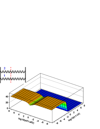
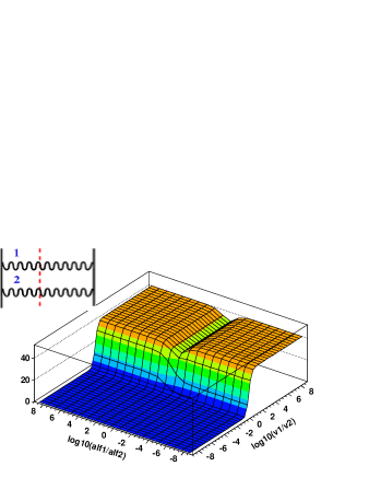
Figure 2: Two double gluon emission ladders

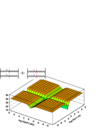
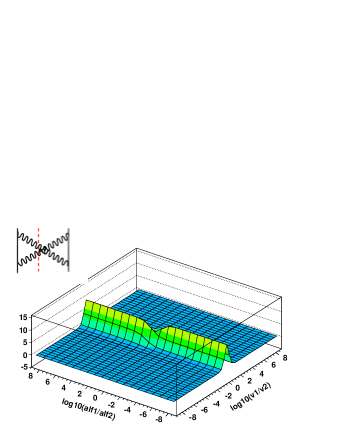
Figure 3: Summarized bremsstrahlung diagram (left), crossed-ladder diagram (right) and their sum (down).

Fig. 3 represents both contributions: from summarized and crossed ladder (upper plots) together with their sum (lower plot). The singly-logarithmic structure, visible on the upper-left plot, disappears completely. The dominant contribution is an infinite “plateau”, with a long “valley” along the line $\alpha_{1}\simeq\alpha_{2}$, This is not an internal infra-red singularity, however, but a leading-log structure. The ladder diagram is not 2PI, but quadratic in the leading-order kernel and therefore requires a soft counterterm to cancel this doubly-logarithmic plateau, see [2]. This counterterm is necessary to construct the NLO kernel and its construction is justified by the CFP scheme. We do not introduce it in this paper, as our aim is to present the universality of gauge cancellations. Therefore we often refer to: “contribution to the NLO kernel” rather than a kernel itself, having in mind that this is not a complete NLO kernel in a strict sense. Despite this dominant LO contribution, in the Fig. 3 one sees no structure in the soft Sudakov limit  (4).

Results of the above numerical exercise can be also understood analytically. Contributions from diagrams in Figs. 1 - 1 in the soft limit are proportional to simple expressions shown in Tab. 1. Two columns in this table refer to two possible different Sudakov limits, with either first or second gluon being soft.

		$\alpha_{1}\rightarrow 0$	$\alpha_{2}\rightarrow 0$
Br1		$C_{F}^{2}\frac{(1+x^{2})}{(1+xy)^{2}}$	$C_{F}^{2}\frac{(1+x^{2})}{(y+x)^{2}}\;x^{2}$
Br2		$C_{F}^{2}\frac{(1+x^{2})}{(1+xy)^{2}}\;x^{2}y^{2}$	$C_{F}^{2}\frac{(1+x^{2})}{(y+x)^{2}}y^{2}$
Bx		$2C_{F}^{2}\frac{(1+x^{2})}{(1+xy)^{2}}\;xy$	$2C_{F}^{2}\frac{(1+x^{2})}{(y+x)^{2}}\;xy$
	SUM	$C_{F}^{2}\left(1+x^{2}\right)$	$C_{F}^{2}\left(1+x^{2}\right)$

Table 1: Contributions from ladders in the Sudakov limit (up to a constant factor)

The common denominator $\frac{1}{(1+xy)^{2}}$ is the (rescaled) square of the virtual quark propagator $\frac{1}{q^{4}}=\frac{1}{((p-k_{1}-k_{2})^{2})^{2}}$ after emitting two gluons. Other factors come from $\gamma$-traces. The last row is the sum of the three, see also the lower plot in Fig. 3. It is finite in the soft Sudakov limit, as the denominator cancels out exactly with the spinorial part of the matrix element squared.

In the above warm-up exercise we have examined in a fine detail how in the NLO kernel calculations, in the axial gauge, quantum interference cancellations do work in practice. In fact they were exactly the same as in QED in axial gauge. Let us now turn to the genuine non-abelian gauge cancellations of the same kind.

3 IR cancellations among genuine non-abelian contributions

In this section we will discuss contributions proportional to $C_{F}C_{A}$ from the diagrams (c-f) of Fig. 1. They are of the genuine non-abelian character, as certified by the presence of $C_{A}$. It is interesting to see how they all “communicate” in the soft Sudakov limit defined below.

We shall start with the overview of the IR cancellations in analytical form and next we shall illustrate them with 2-dimensional plots coming from Monte Carlo numerical exercises. In the following we find useful to use rapidity-related variables $a_{i}$ in order to parametrize phase-space of two gluons:

$$a_{i}=\frac{k_{i\perp}}{\alpha_{i}},\qquad d\Psi=\frac{d\alpha_{1}}{\alpha_{1}}\frac{da_{1}}{a_{1}}d\phi_{1}\,\frac{d\alpha_{2}}{\alpha_{2}}\frac{da_{2}}{a_{2}}d\phi_{2}.$$ (9)

The angular dependence enters only through the relative angle between $k_{1\perp}$ and $k_{2\perp}$ namely $\phi_{12}$, the remaining angle can be integrated out since nothing depends on it.

By the soft Sudakov limit we understand that

$$\begin{cases}\alpha_{i}\rightarrow 0\cr k_{i\perp}\rightarrow 0\end{cases}$$ (10)

while $a_{i}$ is finite. The Sudakov plane in the plots will be parametrized using variables $\log(\alpha_{1}/\alpha_{2})$ and $\log(a_{1}/a_{2})$.

Vg		$C_{F}C_{A}(1+x^{2})\left[\;\frac{u^{2}}{a^{2}}F_{1}+\;\frac{1}{a^{2}}F_{2}\;\right]$
Yg1		$C_{F}C_{A}(1+x^{2})\left[\;\frac{u\cos\phi_{12}-u^{2}}{a^{2}}F_{1}+x\;\frac{\alpha_{2}}{1-x}F_{0}\;\right]$
Yg2		$C_{F}C_{A}(1+x^{2})\left[\;\frac{u\cos\phi_{12}-1}{a^{2}}F_{2}+x\;\frac{\alpha_{1}}{1-x}F_{0}\;\right]$
Bx		$-C_{F}C_{A}(1+x^{2})\;xF_{0}$
	SUM	$C_{F}C_{A}(1+x^{2})\;\frac{u\cos\phi_{12}}{a^{2}}\left(F_{1}+F_{2}\right)$

Table 2: Cancellations of the non-abelian contributions from various diagrams due to gauge invariance (color coherence). Singular part for each diagram is shown in analytical form. Factors $F_{i}$ are relatively mild, see text for their definition.

3.1 General structure of the IR non-abelian cancellations

In Table 2 we summarize the IR cancellations of the non-abelian origin between the two real gluon diagrams contributions to NLO kernel in analytical form. Formulas in Tab. 2 are the leading divergences extracted from two real gluon distributions in a maximally simplified form. Functions $F_{i}$ are relatively mild and defined as follows:

$$\begin{split}&F_{1}=\frac{\alpha_{2}}{\alpha_{1}}\frac{1}{u^{2}}F_{0},\qquad F_{2}=\frac{\alpha_{1}}{\alpha_{2}}u^{2}F_{0},\\ &\sqrt{F_{0}}=\frac{\sqrt{\alpha_{1}\alpha_{2}}u}{\alpha_{1}(1-\alpha_{2})u^{2}+\alpha_{2}(1-\alpha_{1})+2\alpha_{1}\alpha_{2}u\cos\phi_{12}}=\frac{\sqrt{\alpha_{1}\alpha_{2}}a_{1}a_{2}}{q^{2}},\end{split}$$ (11)

where we defined $u=a_{1}/a_{2}$. Moreover we define $a^{2}=1+u^{2}-2u\cos\phi_{12}$, which is up to the $\alpha_{1}\alpha_{2}a_{2}^{2}$ factor, the effective mass of the gluon pair squared $k^{2}=(k_{1}+k_{2})^{2}$. Function $F_{0}$ is proportional to rescaled square of the propagator $1/q^{4}$, which is regular in the soft limit.

The pattern of the IR cancellations in Tab. 2 is manifest.

The most evident singularity is associated with $u/a^{2}$ factor, infinite when the effective mass of the gluon pair is zero. In logarithmic variables this $u/a^{2}$ divergence is seen as a thin infinite ridge along $u=1$. It is a function of $u$ and $\phi_{12}$ only, strongly peaked at $u=1$. In the gluonic vacuum polarization diagram this singularity is dominant. This is, however, a collinear singularity, not a soft one. It remains uncancelled but it is not relevant in our discussion of cancellation of soft singularities. We only mention it to understand the full singularity structure of the diagrams of interest. In Yg1 and Yg2 diagrams the $u/a^{2}$ factor is present, too but the singularity is cancelled out by the numerators.

The factors $uF_{1}$ and $F_{2}/u$ are functions of both $u$ and $\alpha_{1}/\alpha_{2}$. They “soften” the sharp fall of $u/a^{2}$ in the limits $u\rightarrow 0$ and $u\rightarrow\infty$. They are non-zero in the soft Sudakov limit (10), giving rise to a doubly-logarithmic IR divergence. These terms are present in both Vg and Yg diagrams, with opposite signs. This is checked and discussed below in the context of numerical exercises.

In the last row of Tab. 2 the sum of all aforementioned contributions is presented. The terms proportional to $u^{2}F_{1}/a^{2}$ and $F_{2}/a^{2}$ cancel explicitly among diagram with gluonic vacuum polarization and its interference with bremsstrahlung. The remaining factor $F_{1}+F_{2}$ is equal to 1 in the soft Sudakov limit (10), leaving out $u/a^{2}$ factor free from doubly-logarithmic divergences.

Let us stress that this particular cancellation of the doubly logarithmic Sudakov structure of the non-abelian origin in the two-gluon distribution in QCD is usually referred to in the literature as the “color coherence effect”, see for instance ref. [6].

The other IR divergence is caused by the presence of terms $\sim F_{0}$ in diagrams Yg1, Yg2 and Bx, see again Table 2. $F_{0}$ is nonzero along $a_{1}^{2}/a_{2}^{2}=\alpha_{1}/\alpha_{2}$, giving rise to a single-log singularity after phase space integration. This has been discussed already in the case of bremsstrahlung diagrams. Here, however, the analytical cancellation among Yg1, Yg2 and Bx, ensured by $\alpha_{1}+\alpha_{2}=1-x$, occurs in the whole phase-space, not only in the soft limit.

Finally, the only singularities that remain are associated with $u/a^{2}$ term, as discussed before in this section.

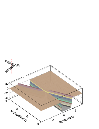
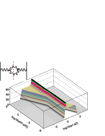
Figure 4: Triple-gluon-vertex diagrams.

3.2 Numerical illustration of IR non-abelian cancellations

In Fig. 4 we show the distribution $f(a_{i},\alpha_{i})$ for two gluons (averaged over the gluon azimuthal angles) for fixed $x=1-\alpha_{1}-\alpha_{2}=0.3$, from gluonic pair production graph (Vg) and its interference with bremsstrahlung (Yg = Yg1+Yg2), see also Tab. 2. Contributions from all diagrams are written explicitly in Tab. 2. In the plots on Figs. 4 - 7 we omit their color coefficients. The gluonic pair production graph (Vg) has a strong peak along the line of equal rapiditites $a_{1}=a_{2}$ originating from $u/a^{2}$ factor (off-shell gluon propagator). In addition, this diagram features in the plot triangular infinite plateau between the lines of the equal rapiditites $a_{1}=a_{2}$ and the line of equal virtualities $v_{1}=v_{2}$. It is exactly this triangular plateau which upon integration leads to $\ln^{2}(1/\delta)$. Note, that in Figs. 4 - 7 we use variables $\log(a_{1}/a_{2})$, contrary to the previous section, where we had $\log(v_{1}/v_{2})$. This is why the line $v_{1}=v_{2}$ is now diagonal in the plots.

Very similar, but with opposite sign, doubly-logarithmic structure is present in the left plot in Fig. 4 from the interference graphs Yg1+Yg2, see also Tab. 2. After adding the contributions from the above diagrams, see Fig. 5, the doubly-logarithmic structure between the lines: $a_{1}=a_{2}$ and $v_{1}=v_{2}$ disappears. What remains, is the single-log singularity, appearing in a familiar shape along the diagonal line of $v_{1}=v_{2}$ (barely visible in the plots of Fig. 4) and collinear singularity represented here as an infinite ridge along the line of equal rapiditites. The latter is associated with zero effective mass of the gluon pair, $k^{2}$.

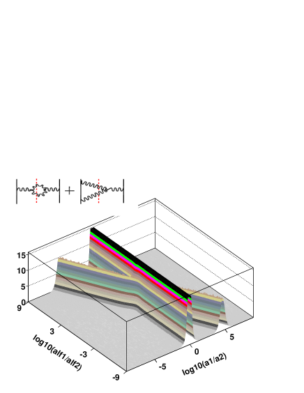
Figure 5: Full cancellation of double-logs between the vacuum polarization diagram and bremsstrahlung-vacuum polarization interference

The above cancellation is the well known “color coherence effect”, see for instance ref. [6]. It reflects the fact that the gluonic pair production graph (Vg) pretends that in the triangular region it is the harder gluon carrying octet color charge which is the “emitter”, with the emission strength $\sim C_{F}C_{A}$. In reality, however, the emitter should be quark carrying triplet color charge, with the almost twice weaker emission strength $\sim C_{F}^{2}$. The role of the interference diagram Yg1+Yg2 is to correct for that and we see this to happen in the plot and in the formulas in Tab. 2. One has to remember that this part of the plot is already populated with the bremsstrahlung diagrams of the previous section proportional to $\sim C_{F}^{2}$.

What still remains in Fig. 5 is a singly-logarithmic structure along the diagonal line $v_{1}=v_{2}$. Its presence is in principle allowed in the doubly-logarithmic Sudakov approximation. A more subtle analysis of the soft limit in QCD shows that it should also vanish and this phenomenon is often referred to as “eikonalization”, see for instance ref. [7, 8]. The job of bringing back the proper soft limit of the two gluon distribution and eliminating remaining single-log structure is done by the crossed bremsstrahlung diagram Bx (in fact its $C_{F}C_{A}$ part), as it is shown in Figs. 6 and 7, see also Tab. 2.

In right hand side of Fig. 6 the crossed-ladder diagram Bx is presented again. On the left hand side of Fig. 6 we show the result of adding the triple-gluon vertex diagrams (Vg+Yg1+Yg2). Both plots have a characteristic single-log structure, seen as an infinite ridge along the diagonal line of equal virtualities $v_{1}=v_{2}$. However, Bx has opposite signs in its $C_{F}C_{A}$ color coefficients. In Fig. 7 we see the result of adding all the above “ non-abelian” diagrams. Bx enters with a minus sign. We see that the singly-logarithmic structure $\sim C_{F}C_{A}$ disappears completely in the soft limit $\alpha_{i}\to 0$. What is still present in the picture is the dominant $1/k^{2}\sim u/a^{2}$ gluon pair mass singularity.

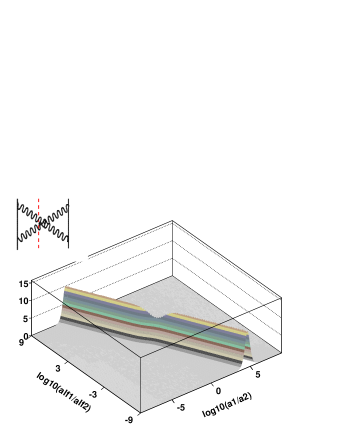
Figure 6: The previous plot (left) and bremsstrahlung diagram (right)

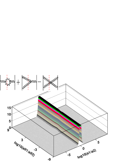
Figure 7: $C_{F}C_{A}$ part of the sum (Vg+Yg $-$ Bx).

The concluding plots are shown in Fig. 8. We presented there Feynman diagrams entering the kernel, both $\sim C_{F}^{2}$ and $\sim C_{F}C_{A}$. In the left plot there are solely amplitude-squared diagrams (Br1, Br2 and Vg) and in the right plot all diagrams including interferences. We see explicitly the crucial role of “color coherence effects” (the interference diagrams) in the cancellation of IR singularities. In the sum of all diagrams of interest we see that remaining structure lies on top of the LO doubly-logarithmic plateau. The plateau does not enter into the NLO kernel. It is cancelled by the counterterm required by the kernel definition, as discussed in Section 2.

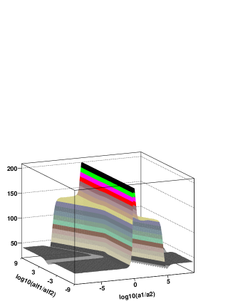
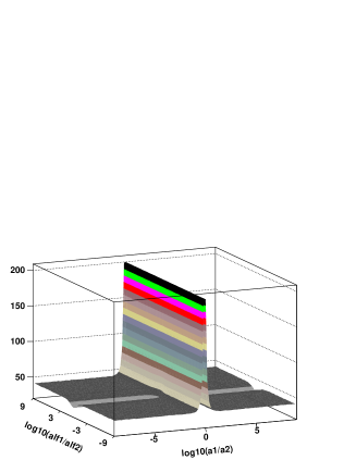
Figure 8: Infra-red cancellations among NLO non-singlet diagrams. Br1, Br2 and Vg (left), Br1, Br2, Bx, Vg, Yg1 and Yg2 (right).

4 Conclusions

We examined the infra-red structure of the diagrams contributing to NLO non-singlet kernel in the unintegrated form.

We have shown the mechanisms of gauge cancellations occurring among different diagrams and the importance of “color coherence effects” for this cancellations.

These effects in soft Sudakov limit are examined/discussed in both analytical and numerical form.

Acknowledgments
We would like to thank Stanisław Jadach, Maciej Skrzypek and Boris Ermolaev for many useful discussions during the preparation of this work.

References

-
[1]
L.N. Lipatov, Sov. J. Nucl. Phys. 20 (1975) 95;
V.N. Gribov and L.N. Lipatov, Sov. J. Nucl. Phys. 15 (1972) 438;
G. Altarelli and G. Parisi, Nucl. Phys. 126 (1977) 298;
Yu. L. Dokshitzer, Sov. Phys. JETP 46 (1977) 64. - [2] S. Jadach and M. Skrzypek, report IFJPAN-IV-09-3, to appear in these proceedings. arXiv:0905.1399 [hep-ph].
- [3] G. Curci, W. Furmanski, and R. Petronzio, Nucl. Phys. B175 (1980) 27.
- [4] R. K. Ellis, H. Georgi, M. Machacek, H. D. Politzer, and G. G. Ross, Phys. Lett. B78 (1978) 281.
- [5] S. Jadach, Comput. Phys. Commun. 152 (2003) 55–100, physics/0203033.
- [6] Y. Dokshitzer, V. Khoze, A. Mueller, and S. Troyan, Basics of Perturbative QCD. Editions Frontieres, 1991.
- [7] D. R. Yennie, S. Frautschi, and H. Suura, Ann. Phys. (NY) 13 (1961) 379.
- [8] J. Frenkel, J. G. M. Gatheral, and J. C. Taylor, Nucl. Phys. B228 (1983) 529.