Parameter estimation for signals from compact binary inspirals injected into LIGO data
Abstract
During the fifth science run of the Laser Interferometer Gravitational-wave Observatory (LIGO), signals modelling the gravitational waves emitted by coalescing non-spinning compact-object binaries were injected into the LIGO data stream. We analysed the data segments into which such injections were made using a Bayesian approach, implemented as a Markov-chain Monte-Carlo technique in our code SPINspiral. This technique enables us to determine the physical parameters of such a binary inspiral, including masses and spin, following a possible detection trigger. For the first time, we publish the results of a realistic parameter-estimation analysis of waveforms embedded in real detector noise. We used both spinning and non-spinning waveform templates for the data analysis and demonstrate that the intrinsic source parameters can be estimated with an accuracy of better than 1–3% in the chirp mass and 0.02–0.05 (8–20%) in the symmetric mass ratio if non-spinning waveforms are used. We also find a bias between the injected and recovered parameters, and attribute it to the difference in the post-Newtonian orders of the waveforms used for injection and analysis.
pacs:
02.50.-r, 02.70.Uu, 04.30.Tv, 04.80.Nn, 95.85.Sz1 Introduction
The inspiral of stellar-mass compact binaries via gravitational-wave emission is among the most promising gravitational-wave sources for ground-based laser interferometers, such as LIGO [1, 2] and Virgo [3]. If such a binary contains a black hole, it is expected to be spinning moderately [4]. A spinning black hole causes the binary orbit to precess, introducing phase and amplitude modulations in the gravitational-wave signal. Accounting for these effects improves the detection efficiency and also improves the accuracy of the parameter estimation on the signal. The accuracy with which the binary parameters can be determined is of significant astrophysical interest; the effect of spin on this accuracy is described in an initial parameter study [5].
We have developed a code called SPINspiral which implements a Markov-chain Monte-Carlo (MCMC) technique [6] to compute the posterior probability-density functions (PDFs), or simply posteriors, of the source parameters of binary inspirals with spinning components. SPINspiral is a modification of an earlier parameter-estimation code for analysis on binaries without spin [7, 8]. In addition to including post-Newtonian gravitational waveforms with a single spinning object [9], we have also implemented a number of improvements designed to make the parameter-space exploration more efficient [10, 11].
During the fifth LIGO science run (S5) [12], modelled gravitational-wave signals from compact binary coalescences with non-spinning members were injected into LIGO data, in order to test the detection pipeline [13, 14]. These hardware injections were made for a variety of masses and signal-to-noise ratios (SNRs). The data sets thus obtained provide the most realistic approximations to actual observed gravitational-wave signals and form an ideal testbed for our parameter-estimation code. In particular, the noise realisation is that of the actual interferometers, as opposed to the Gaussian noise we have used in previous studies, and the injected waveforms are of a higher (2.0) post-Newtonian (pN) order.
In this paper, we present the results of the parameter-estimation analysis with SPINspiral of three such hardware injections; the signals of binary inspirals of black-hole–neutron-star (BH-NS), NS-NS and BH-BH binary inspirals. In section 2 we briefly describe our MCMC code. Section 3 contains the results of our analyses, where we show that we typically recover the chirp mass to a few percent accuracy, while in some cases we find a bias between the injected and recovered values of mass and spin parameters. We conclude these proceedings with a discussion of these results in section 4.
2 Implementation of MCMC technique
In this section, we briefly describe the main features of our MCMC code SPINspiral for binary inspirals with spin, including the waveform used, the likelihood computation and the way we choose our priors and perform jump proposals. More details can be found in [10] and in a forthcoming paper [11].
2.1 Waveform
We use a waveform that takes into account post-Newtonian (pN) expansions up to the 1.5-pN order in phase and is restricted to the Newtonian order in amplitude. The waveform includes the simple-precession prescription [9]. This choice of waveform template allows us to investigate the first-order effects of spin (spin-orbit coupling), as long as only one binary member has spin. In comparison to higher-order pN, double-spin waveforms, where the spin-spin interaction is taken into account, this waveform can be computed analytically and has a parameter space with lower dimensionality, so that the computational cost per iteration is lower and the number of iterations needed for convergence is smaller.
The waveform for a binary inspiral with one spinning object is described by 12 parameters: the chirp mass , symmetric mass ratio , the constant, dimensionless spin magnitude , the constant angle between spin and orbital angular momentum , the luminosity distance and sky position , , the time, orbital phase and precession phase at coalescence , , , and two angles that define the direction of the total angular momentum of the binary: and . Each waveform template is computed in the time domain, and then windowed and Fourier transformed. The calculation of the likelihood (1), which measures how well a model waveform matches the data, is carried out in the frequency domain.
2.2 Computation of the likelihood
We follow a Bayesian approach to infer the posterior probability-density functions (PDFs) of the twelve parameters that describe our waveform. We can compute the likelihood for a model waveform with parameters and data set as measured by a detector using
| (1) |
The tildes indicate that both and are expressed in the frequency domain, and is the one-sided noise power-spectral density. Assuming that the noise of different interferometers is independent, the expression for the posterior PDF given the data from a coherent network of interferometers generalises to
| (2) |
where is the prior distribution of the parameters. Further details on Bayesian inference and its application to a coherent network of detectors can be found in [7].
2.3 Prior distributions
We use prior distributions that are uniform in , , , , and in the linear scales of the remaining parameters. SPINspiral is designed to work as a follow-up analysis tool, to be used after a gravitational-wave trigger has been detected and identified as a binary-inspiral candidate. Hence, we can rely on some prior information from the detection trigger, in particular for the chirp mass and time of coalescence of the trigger. We start our Markov chains from a chirp-mass value chosen randomly from a Gaussian distribution with a width of 0.25 111This value is somewhat arbitrary, and relatively large. If chains can converge from such distant initial values, they are guaranteed to converge when started from the value returned by the detection pipeline. around , with a value for from a Gaussian that is 0.1 s wide around , and randomly from the whole prior distribution in all other parameters.
The prior ranges used in this study for the 12 parameters are between ; ; ; ; ; ; ; ; ; ; ; and . We use these broad, flat priors to keep our study general. However, when additional information becomes available (for instance the time and sky location of a gamma-ray burst during an externally-triggered search), the priors can be restricted accordingly.
2.4 Jump proposals
Bayes’ theorem allows us to combine the model’s prior distribution and likelihood and derive the PDF containing the information about the parameters given the data. We use stochastic Monte-Carlo integration for this purpose, implemented in a Markov-chain Monte-Carlo (MCMC) scheme (e.g. [6]). The Metropolis algorithm used here requires the specification of a proposal distribution, which defines how (and how efficiently) the parameter space is explored. We use an adaptive scheme to regulate the proposed jump size (e.g. [15]) with a target acceptance rate of about 25%.
Typically we propose approximately 10% of our MCMC jumps for each parameter individually. The other jump proposals are done in all 12 parameters at once. To make these all-parameter updates more efficient, we use the covariance matrix that the code computes from previous iterations to guide the jump proposals. More details of our jump proposals are described in section 2.5 of [10] and in [11].
In order to both explore all of the wide prior ranges of our parameter space and at the same time sample the much smaller regions of interest in detail, we use a technique that is known as parallel tempering. We run several (typically ) Markov chains in parallel, each with a different ‘temperature’ assigned. While hot chains can explore a larger part of the parameter space, only data from the coolest chain, which samples the regions of interest in detail, is used to generate the posterior PDFs. Our implementation of parallel tempering is described in more detail in section 2.6 of [10] and in [11].
3 MCMC analysis of hardware injections
During the fifth LIGO science run (S5), which ended in October 2007, modelled gravitational-wave signals from compact binary coalescences (CBCs) were injected into LIGO data to test the CBC detection pipeline. The signals were introduced in the detector by physically moving the mirrors of the interferometer, according to precomputed simulated 2.0-pN, inspiral waveforms. Such hardware injections were done for a variety of binary-component masses and for different signal-to-noise ratios (SNRs).
Most of these hardware injections had non-spinning components, and were done simultaneously for the LIGO 4-km interferometers H1 (Hanford) and L1 (Livingston), and 2-km interferometer H2. However, the signal injected into each detector was that of an optimally oriented (‘face-on’) source located exactly overhead that detector. Hence, the injections were not coherent, i.e., there is no predefined choice of sky location, orientation and distance for the source that is consistent in all interferometers.
Since the SNR in the H2 detector is typically about half of that in the other two LIGO interferometers, adding the H2 data to that of H1 and L1 in our coherent analysis raises the network SNR by only about 6%, while it increases the computational cost by 50%. The CPU time scales linearly with the number of detectors included in the analysis. We therefore ran our parameter estimation with the data from the H1 and L1 only.222Strictly speaking, using data from both H1 and H2 would invalidate Eq. 2, since the noise realisations of the two detectors are not independent.
In order to accurately sample the parameter space in our MCMC runs, we typically need to accumulate a few million iterations. A run with two detectors and the waveform described in section 2.1 takes about a week to compute iterations on a single 2.8 GHz CPU, when five parallel-tempering chains are used.
3.1 A black-hole–neutron-star injection
In this section, we present our analysis of the hardware injection of the signal from a non-spinning inspiral of a 10.0 BH and a 1.4 NS at a distance of 50 Mpc. We used 7.0 s of data from the H1 and L1 interferometers for the parameter estimation. We ran the analysis both allowing the BH spin to be determined (spMCMC) and assuming that no spin was present (nsMCMC).
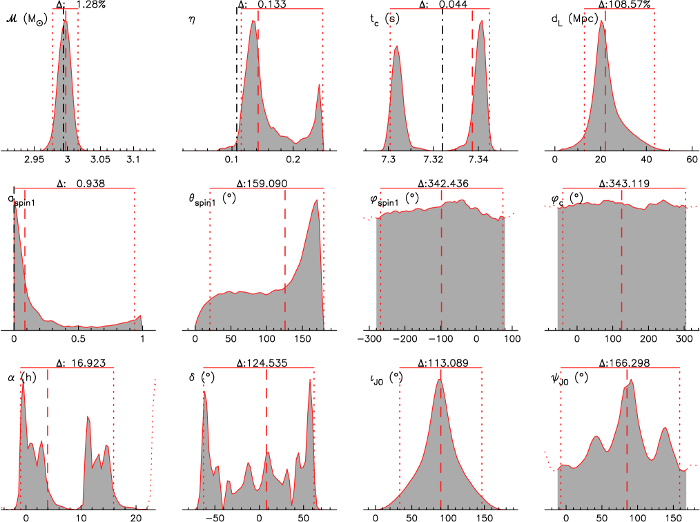
Figure 1 shows the marginalised PDFs from the spMCMC analysis. Each of the panels in the figure contains the posterior PDF for one of the twelve parameters. The railing of the PDF for against the lower limit of the prior range is consistent with the non-spinning nature of the injection. The 2- probability ranges shown in the figure are defined as the smallest range that contains 95.45% of the PDF.

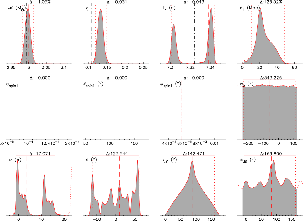
Figure 2 contains the same information as figure 1, but for the nsMCMC analysis. Hence, the three panels , and are empty. The medians and 2- ranges for the main parameters in both the spMCMC and nsMCMC analyses are summarised in table 1. We see clearly that the symmetric mass ratio is overestimated in both parameter-estimation runs. A discussion of a possible explanation of the biases in this and the next analyses can be found in section 4. In addition to that, the PDF for is bimodal for the spMCMC run, but not for the nsMCMC run. This degeneracy seems to be introduced by the correlations between and the spin parameters [5]. These correlations can account for the larger uncertainties in the determination of and in the spMCMC analysis.

-
med. 2- range med. 2- range med. 2- range Injection 2.994 — 0.107 — 0.00 — spMCMC 2.998 2.978 – 3.016 0.143 0.115 – 0.248 0.08 0.00 – 0.94 nsMCMC 2.999 2.983 – 3.014 0.134 0.119 – 0.150 — —
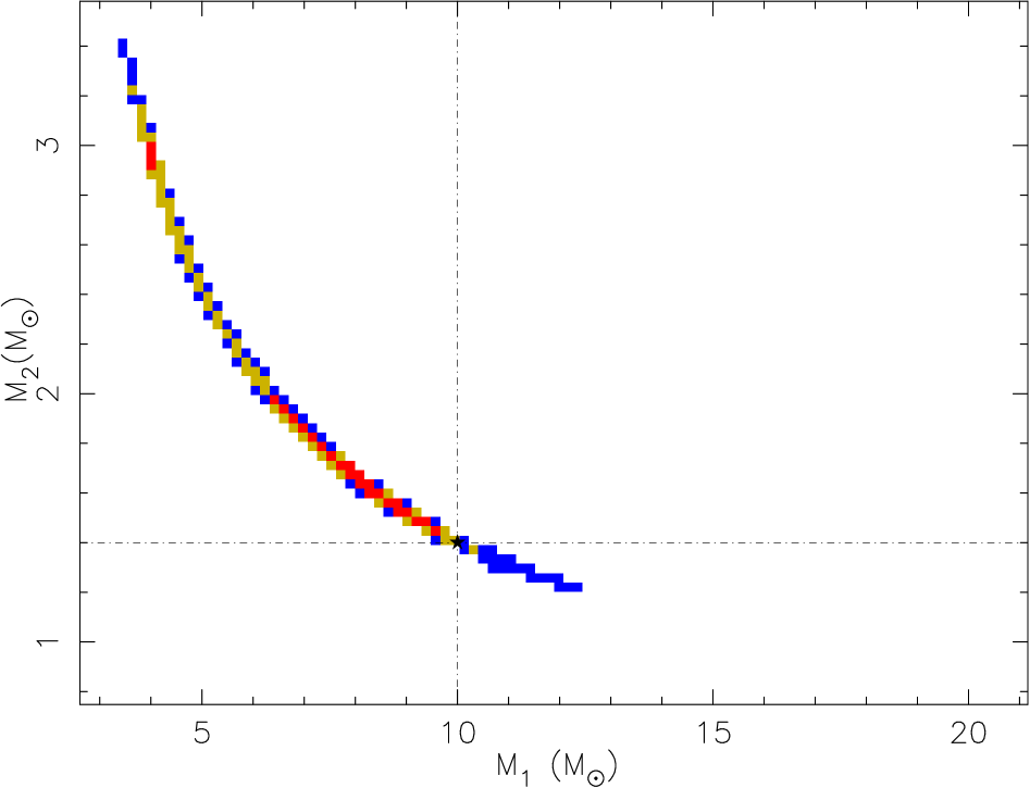
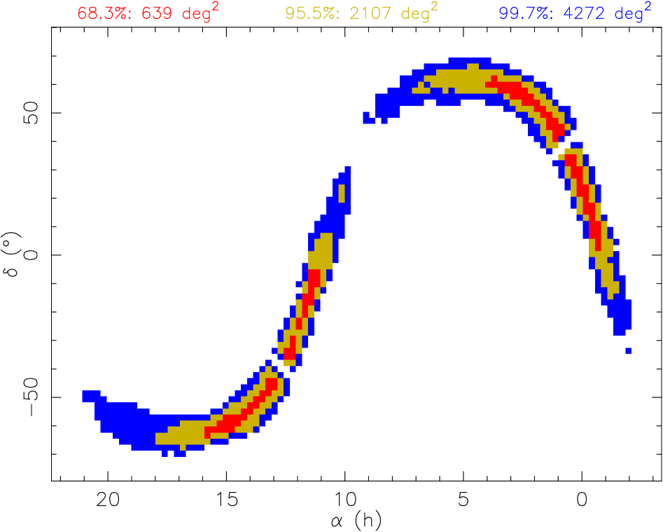
Figure 3 shows two-dimensional PDFs from the spMCMC analysis of the BH-NS inspiral. These PDFs are rather narrow and the surface contained in them is much smaller than suggested by the corresponding one-dimensional PDFs. Figure 3a shows a very thin arc in the - plane, the width of which is determined by the uncertainty in the chirp mass, and whose length is set by the much larger uncertainty in . The 2D PDF in figure 3b represents a great circle in the sky, as expected for a coincident but non-coherent injection. The gaps in the ‘ring’ represent areas where the probability density is low, due to a smaller volume of support in other extrinsic parameters, such as the binary orientation and distance [16].


3.2 A neutron-star–neutron-star injection
We analysed the hardware injection that was performed for the signal of the binary inspiral of two 1.4 neutron stars (NSs) at a distance of 40 Mpc, using 14.0 s of data from each of the detectors H1 and L1. The results of both the spMCMC and nsMCMC analyses for this injection are summarised in table 2. In this case of an equal-mass injection, we cannot overestimate the value of . Instead, we find that the chirp mass is underestimated in the nsMCMC run, but not in the spMCMC run. It is possible that an overestimation of in the spMCMC run mimics the effect of the underestimation of in the nsMCMC run. When compared to table 1, we see that the median for is significantly higher here, indicating that this parameter does not reach the lower limit of the prior as much as is the case for the PDF of the BH-NS analyses in figure 1.
-
med. 2- range med. 2- range med. 2- range Injection 1.219 — 0.250 — 0.00 — spMCMC 1.218 1.211 – 1.229 0.219 0.057 – 0.250 0.41 0.00 – 0.80 nsMCMC 1.214 1.211 – 1.216 0.238 0.201 – 0.250 — —
3.3 A black-hole–black-hole injection
The LSC did a hardware injection into LIGO data for a 3.0+3.0 , non-spinning BH-BH inspiral at a distance of 40 Mpc. We used 8.0 s of data from both H1 and L1 for the analysis. A summary of the results of the spMCMC and nsMCMC analyses is listed in table 3. As for the NS-NS result in section 3.2, we find that the chirp mass is underestimated for the nsMCMC run, but not for the spMCMC run. In the spMCMC run, the value for is again higher than the recovered value in the analysis of the BH-NS signal, and here this parameter is actually slightly overestimated. In section 4 we discuss a possible explanation for these biases.
-
med. 2- range med. 2- range med. 2- range Injection 2.612 — 0.250 — 0.00 — spMCMC 2.608 2.576 – 2.634 0.236 0.153 – 0.250 0.35 0.03 – 0.73 nsMCMC 2.588 2.576 – 2.595 0.240 0.212 – 0.250 — —
4 Conclusions and future work
In these proceedings, we showed that our MCMC code SPINspiral can provide parameter estimation for binary-inspiral signals under realistic circumstances. Whereas in [5] we tested the parameter-estimation code on software injections that we performed ourselves in Gaussian noise and with a fairly high SNR (17 for the network), the examples in this paper show that our code is capable of the post-detection follow-up analysis it was designed for. The hardware injections were performed with a different waveform family, with relatively low SNRs and in observed LIGO detector data. We demonstrated that our parameter-estimation code can use the information that could be available from a detection trigger and return the posterior-density functions for the physical parameters. The results for the weaker signals in our analysis suggest that SPINspiral is able to analyse even the weakest signals that will be detected by the CBC detection pipeline.
Because the hardware injections were done non-coherently, the results presented in section 3 are of limited interest for most parameters. The posterior PDFs for the sky location should be a great circle, which is what we find. However, the inclination should indicate a ‘face-on’ system, whereas our PDFs prefer an ‘edge-on’ system, either because of the shape of the prior distribution, or more strongly than that. The recovered PDFs for the phases and , and the polarisation angle are practically meaningless here. Because the hardware injections were overhead in each detector, there is no consistent solution for , and the recovered distance is smaller than the distance of the injection.
The results for the mass and spin parameters are much more interesting. In several cases, our PDFs for some of these parameters are offset from the injection values. The main reason for this is most likely the systematic error that is introduced by the difference in waveforms used for the injection (2.0-pN) and the parameter estimation (1.5-pN). This difference may give rise to a difference of gravitational-wave cycles during the inspiral in the LIGO band [17]. It seems reasonable that parameters like and should be changed significantly in order to compensate for this effect.
In the BH-NS inspiral in section 3.1 we clearly overestimate in both the spMCMC and nsMCMC runs. In the other two analyses, cannot be overestimated, and we find biases in or instead, which may be due to the correlations between these parameters. On the other hand, we expect that the statistical accuracies which we find in the parameter estimation are representative, and that these accuracies will improve once the systematic biases are dealt with.
To achieve this improvement, part of our current work focuses on the implementation of a more realistic waveform template. SPINspiral is now able to use a 3.5-pN template from the LSC Algorithm Library [18], which allows for the spins of both binary members [19]. Our first results indeed show an improvement in accuracy, especially in the mass parameters, due to the removal of the systematic errors mentioned here (using the same waveform family for injections and parameter-estimation templates), and due to the higher post-Newtonian order used [16].
Our second focus of code development is aimed at adding SPINspiral to the CBC follow-up pipeline. This will allow many people to run the code — and to run it automatically — on triggers that are plausible inspiral events (either from gravitational waves, or from hardware injections). Inclusion of SPINspiral in the pipeline will increase the number of tests we can perform, and make these tests as realistic as possible, optimally approximating the ‘real’ process of gravitational-wave detection and analysis.
Acknowledgements
This work is partially supported by a Packard Foundation Fellowship and a NSF Gravitational Physics grant (PHY-0653321) to VK; NSF Gravitational Physics grant PHY-0553422 to NC. Computations were performed on the Fugu computer cluster funded by NSF MRI grant PHY-0619274 to VK.
References
References
- [1] A. Abramovici et al. LIGO - The Laser Interferometer Gravitational-Wave Observatory. Science, 256:325–333, April 1992.
- [2] Waldman, S. J. (for the LIGO Science Collaboration). Status of ligo at the start of the fifth science run. Class. Quant. Grav., 23(19):S653–S660, 2006.
- [3] F. Acernese et al. Status of virgo detector. Class. Quant. Grav., 24(19):S381–S388, 2007.
- [4] K. Belczynski, R. E. Taam, E. Rantsiou, and M. van der Sluys. Black Hole Spin Evolution: Implications for Short-Hard Gamma-Ray Bursts and Gravitational Wave Detection. ApJ, 682:474–486, July 2008.
- [5] M. V. van der Sluys, C. Röver, A. Stroeer, V. Raymond, I. Mandel, N. Christensen, V. Kalogera, R. Meyer, and A. Vecchio. Gravitational-Wave Astronomy with Inspiral Signals of Spinning Compact-Object Binaries. ApJ, 688:L61–L64, December 2008.
- [6] W. R. Gilks, S. Richardson, and D. J. Spiegelhalter. Markov chain Monte Carlo in practice. London/Boca Raton, Fl.: Chapman & Hall/CRC, 1996.
- [7] C. Röver, R. Meyer, and N. Christensen. Coherent Bayesian inference on compact binary inspirals using a network of interferometric gravitational wave detectors. Phys. Rev. D, 75(6):062004, March 2007.
- [8] C. Röver. PhD thesis, The University of Auckland, 2007.
- [9] T. A. Apostolatos, C. Cutler, G. J. Sussman, and K. S. Thorne. Spin-induced orbital precession and its modulation of the gravitational waveforms from merging binaries. Phys. Rev. D, 49:6274–6297, June 1994.
- [10] M. van der Sluys, V. Raymond, I. Mandel, C. Röver, N. Christensen, V. Kalogera, R. Meyer, and A. Vecchio. Parameter estimation of spinning binary inspirals using Markov chain Monte Carlo. Class. Quant. Grav., 25(18):184011, September 2008.
- [11] M. van der Sluys, V. Raymond, I. Mandel, V. Kalogera, C. Röver, N. Christensen, and A. Vecchio. In preparation.
- [12] D. Sigg and the LIGO Science Collaboration. Status of the LIGO detectors. Class. Quant. Grav., 23:51, April 2006.
- [13] Gouaty R for the LIGO Scientific Collaboration. Detection confidence tests for burst and inspiral candidate events. Class. Quant. Grav., 25(18):184006, September 2008.
- [14] LIGO Scientific Collaboration: B. P. Abbott. Search for gravitational-wave bursts in the first year of the fifth LIGO science run. ArXiv e-prints, April 2009.
- [15] Y. F. Atchadé and J. S. Rosenthal. On adaptive Markov chain Monte Carlo algorithms. Bernoulli, 11(5):815–828, 2005.
- [16] V. Raymond, M. V. van der Sluys, I. Mandel, V. Kalogera, C. Roever, and N. Christensen. Degeneracies in Sky Localisation Determination from a Spinning Coalescing Binary through Gravitational Wave Observations: a Markov-Chain Monte-Carlo Analysis for two Detectors. Class. Quant. Grav., in press, December 2009.
- [17] Luc Blanchet. Gravitational radiation from post-newtonian sources and inspiralling compact binaries. Living Reviews in Relativity, 9(4), 2006.
- [18] LIGO Scientific Collaboration. The LSC Algorithm Library. February 2007.
- [19] A. Buonanno, Y. Chen, and M. Vallisneri. Detecting gravitational waves from precessing binaries of spinning compact objects: Adiabatic limit. Phys. Rev. D, 67(10):104025, May 2003.