Be Star Disk Models in Consistent Vertical Hydrostatic Equilibrium

Abstract

A popular model for the circumstellar disks of Be stars is that of a geometrically thin disk with a density in the equatorial plane that drops as a power law of distance from the star. It is usually assumed that the vertical structure of such a disk (in the direction parallel to the stellar rotation axis) is governed by the hydrostatic equilibrium set by the vertical component of the star’s gravitational acceleration. Previous radiative equilibrium models for such disks have usually been computed assuming a fixed density structure. This introduces an inconsistency as the gas density is not allowed to respond to temperature changes and the resultant disk model is not in vertical, hydrostatic equilibrium. In this work, we modify the bedisk code of Sigut & Jones (2007) so that it enforces a hydrostatic equilibrium consistent with the temperature solution. We compare the disk densities, temperatures, H$\alpha$ line profiles, and near-IR excesses predicted by such models with those computed from models with a fixed density structure. We find that the fixed models can differ substantially from the consistent hydrostatic models when the disk density is high enough that the circumstellar disk develops a cool ($T\lesssim 10,000\;$K) equatorial region close to the parent star. Based on these new hydrostatic disks, we also predict an approximate relation between the (global) density-averaged disk temperature and the $T_{\rm eff}$ of the central star, covering the full range of central Be star spectral types.

1 Introduction

Be stars are non-supergiant B stars that currently show, or have shown in the past, emission in one or more of the hydrogen Balmer lines, typically H$\alpha$ (Porter & Rivinus, 2003). Other common characteristics of Be stars include an infrared excess (Waters, 1986) and linear continuum polarization at the level of approximately one percent (Waters & Marlborough, 1992). These observations can be explained by the presence of a non-spherical distribution of circumstellar material surrounding the central B star (Wood et al., 1997). Be stars have recently been resolved interferometrically in the optical (Quirrenbach et al., 1993; Tycner et al., 2005, 2006) to conclusively show that this circumstellar material is in the form of a thin equatorial disk, a form originally championed by Poeckert & Marlborough (1978). Typically the spectra of Be stars are consistent with this thin disk in near Keplerian rotation in which the equatorial density drops as a power-law in radius. In such models, the vertical structure of the gas (perpendicular to the disk) is often assumed to be in isothermal hydrostatic equilibrium. In this case, the overall disk density, expressed in cylindrical co-ordinates $(R,Z)$ where the $Z$ direction is parallel to the rotation axis of the star, is

$$\rho(R,Z)=\rho_{o}\left(\frac{R_{*}}{R}\right)^{n}e^{-\left(\frac{Z}{H}\right)^{2}}\;.$$ (1)

Here $R_{*}$ is the stellar radius, $\rho_{o}$ is the density of the inner edge of the disk in the equatorial plane (often termed the “base density” of the disk), and $H$ is a vertical scale-height that depends upon the distance, $R$, the stellar mass, $M_{*}$, and a disk temperature, $T_{o}$, assumed valid for all $Z$ at that distance. Such a density model balances the vertical component of the star’s gravitational acceleration (parallel to the rotation axis) with the pressure set by the temperature $T_{o}$. If $T_{o}$ is a constant for all radial distances, the weakening of the vertical gravitational acceleration with $R$ causes $H\propto R^{3/2}$ and the disk flares with increasing distance. Here $\rho_{o}$ and the power-law index, $n$, are the parameters that determine the overall density of the disk (together with the assumed value for $T_{o}$ which is often simply set to a constant fraction of the $T_{\rm eff}$ of the central star). Typically one fixes these parameters by comparing to the observational constraints cited above. By matching the infrared excess of a wide sample of Be stars, Waters et al. (1987) and Dougherty et al. (1994) find power-law indexes in the range of $n=2.0$ to $5.0$. Theoretically, Porter (1999) notes that an isothermal, viscous disk requires $n\geq 3.5$ for outflow, and Jones, Sigut & Porter (2007) find that a hydrodynamical simulation of outflowing viscous disks in which the thermal structure of the disk is taken into account (following Jones, Sigut & Marlborough, 2004) predicts $n$ in the range of $3.0$ to $3.5$ in the inner portion of the disk, $R\lesssim 10\,R_{*}$, where hydrogen spectrum likely forms.

While empirically probing the temperature structure within Be star disks is a difficult observational challenge, several theoretical models of the temperature structure of such disks now exist (Carciofi & Bjorkman, 2006; Sigut & Jones, 2007). Typically, for low densities, the disks are nearly isothermal. However, as the density rises (i.e. as $\rho_{o}$ is increased), a cool equatorial region develops close to the star and the disk gas becomes far from isothermal in the vertical direction, even at a single $R$. Such models are fundamentally inconsistent because the derived temperature structure can no longer be consistent with the assumption of a vertically isothermal gas as required by Eq. 1. As observational diagnostics can be very sensitive to the gas density in the disk, such an inconsistency may have observational consequences in terms of the predicted emission line profiles and strengths, the predicted IR excess, and the predicted linear polarization signature. For example, Carciofi & Bjorkman (2006) suggest that the fundamental limitation to Waters (1986) technique for determining disk density from the slope of the IR continuum is the a priori assumption of disk geometry via the adoption of a constant disk opening angle.

It is the purpose of the present work to eliminate this inconsistency between the temperature and density structure of the disk. Radiative equilibrium models are constructed in which the vertical disk density structure is in a hydrostatic equilibrium consistent with the computed temperature distribution.

2 Theory

We assume an axisymmetric disk described by the cylindrical co-ordinates $(R,Z)$. We shall also assume that the disk density in the equatorial plane ($Z=0$) is a known function of $R$ of the form

$$\rho(R,0)=\rho_{o}\,\left(\frac{R_{*}}{R}\right)^{n}\;,$$ (2)

where $R_{*}$ is the stellar radius; $\rho_{o}$ and the power-law index $n$ are free parameters that fix the density structure of the disk. Thus at any location $R$, the density $\rho(R,0)$ is known, and we shall denote this density simply as $\rho(0)$. If the gas at this location is in vertical hydrostatic equilibrium, then the vertical pressure gradient must satisfy the equation of hydrostatic equilibrium,

$$\frac{dP}{dz}=-\rho\,g_{\rm z}\;.$$ (3)

Here $g_{\rm z}$ is the vertical (or z-component) of the star’s gravitational acceleration at location $R$, namely

$$g_{z}=GM_{*}\,\frac{Z}{(R^{2}+Z^{2})^{3/2}}\;,$$ (4)

where $M_{*}$ is the mass of the central star. In all cases, $\rho_{o}$ in Eq. 2 is so small that the mass of the disk is completely negligible compared to that of the star. The pressure can be eliminated from the hydrostatic equation as the gas is assumed to obey the perfect gas law,

$$P=\frac{\rho}{\mu m_{H}}\,kT\;.$$ (5)

This introduces the vertical temperature distribution into the problem. In this equation, $P$, $\rho$, $T$, and $\mu$ are functions of $Z$ (the mean-molecular weight, $\mu$, depends on $Z$ because it is determined by the ionization state of the gas). Using the perfect gas law to eliminate the pressure from Eq. 3, and using Eq. 4, we find that

$$\frac{1}{\rho}\,\frac{d\rho}{dz}=-\alpha(Z)\,\frac{Z}{(R^{2}+Z^{2})^{3/2}}\;,$$ (6)

where $\alpha(Z)$ is the function

$$\alpha(Z)=GM_{*}\,\frac{\mu(Z)m_{\rm H}}{kT(Z)}\;.$$ (7)

Using the boundary condition that the density at $Z=0$ is equal to $\rho(0)$, Eq. 6 can be numerically integrated assuming that the functions $T(Z)$ and $\mu(Z)$ are known. Typically a numerical solution is required as the temperature $T(Z)$ is available only at a fixed number of vertical grid points via a radiative equilibrium solution. In the sections to follow, we shall use the bedisk code of Sigut & Jones (2007) to compute the thermal structure of several Be disks so that the vertical hydrostatic equation can be numerically integrated at each distance from the star.

The analytic solution of Eq. 6, seen in Eq. 1, is obtained when the vertical temperature variation can be replaced by a constant temperature $T_{o}$ (with the mean-molecular weight also assumed to be a constant, $\mu_{o}$). In this case, Eq. 7 is just the parameter $\alpha_{o}$, and Eq. 6 is readily integrated to give

$$\rho(Z)=\rho(0)\,e^{-\alpha_{o}\left(\frac{1}{R}-\frac{1}{\sqrt{R^{2}+Z^{2}}}\right)}\;.$$ (8)

In the case of a geometrically thin disk in which $Z/R\ll 1$, applicable to the Be stars, this result simplifies to

$$\rho(Z)=\rho(0)e^{-\frac{\alpha_{o}}{2R}\left(\frac{Z}{H}\right)^{2}}\;.$$ (9)

Comparing to Eq. 1, the scale-height H is given by

$$H=\sqrt{\frac{2R^{3}}{\alpha_{o}}}\;,$$ (10)

which gives the cited $H\propto R^{3/2}$ disk flaring with distance. Thus the assumption of vertically isothermal gas in the Be disk is required to reproduce the density structure of Eq. 1.

3 Computational Procedure

To obtain the temperature structure of various Be star disk models, we use the bedisk code of Sigut & Jones (2007). This code has been successfully used to interpret a wide range of Be star observational signatures (for example, see Tycner et al., 2008; Jones et al., 2008, 2009). The bedisk code solves the radiative equilibrium problem for the disk gas by balancing the heating and cooling rates computed for a user-specified set of atomic models. Energy input to the disk is assumed to come from the radiation of the central star. This photoionizing radiation field is represented as a sum of the direct component from the central star and the diffuse component from the disk itself, which is treated by the on-the-spot (OTS) approximation (Osterbrock, 1989). Sigut & Jones (2007) present results for a direct (but still approximate) treatment of the diffuse component to demonstrate its affect on the thermal structure of the disk. They find that even for a dense disk with $\rho_{o}=5\cdot 10^{-11}\;\rm g\,cm^{-3}$ and an $R^{-2.5}$ radial drop-off, the additional heating provided by the diffuse component increases the temperature in the inner equatorial plane by only 10-20% and conclude that the OTS approximation gives good results.

Limb darkening of the central star is accounted for in the direct photoionizing radiation field, but the gravitational darkening and geometric distortion implied by rapid rotation is yet to be implemented. Heating of the gas is via photoionization and collisional excitation. Cooling of the gas is via recombination and collisional de-excitation. The atomic level populations required to compute the heating and cooling rates were found by solving the requisite statistical equilibrium equations. The transfer of line radiation is handled through the escape probability approximation. See Sigut & Jones (2007) for further details.

To achieve a solution that is both in radiative equilibrium and in a vertical hydrostatic equilibrium consistent with the temperature structure, some modification to the bedisk code is required. The initial density distribution is simply that of Eq. 1. bedisk then obtains the disk temperatures on a fixed grid specified by the cylindrical coordinates $(R_{i},Z_{ij})$, with $i=1,2,\ldots,n_{r}$ and $j=1,2,\ldots,n_{z}$ where $R_{i+1}>R_{i}$ and $Z_{i,j+1}>Z_{i,j}$. The solution starts closest to the star (at $i=1$) and statistical and radiative equilibrium is solved for each $Z_{1,j}$ for $j=n_{z},n_{z}-1,\ldots,1$, i.e. by proceeding down towards the equatorial plane. Then Eq. 6 is numerically integrated using the density in the equatorial plane as the boundary condition. As a result of this integration, the total gas density for $i=1$ and all $j=1,2,\ldots,n_{z}$ is updated. As the gas density at each $Z_{1,j}$ has been changed, radiative equilibrium must be resolved to obtain a new temperature distribution. This process is iterated until the maximum fractional change in the gas density drops below 1%. Once this has happened, the calculation proceeds to the next radial distance in the disk, $i=2$, and so on.

If, on average, $N_{\rho}$ density iterations are required to meet the convergence tolerance, then the entire calculation for consistent vertical hydrostatic equilibrium takes $N_{\rho}$ times that required for the radiative equilibrium solution with the fixed density structure of Eq. 1. As $N_{\rho}\approx 5-10$, a significant lengthening of the execution time of bedisk occurs. Finally, we have found that the various iterative estimates for the density often tend to oscillate around the true value, and it is generally advantageous to update the grid densities with a relaxed estimate that is the average of the old value and the new predicted estimate.

4 Results

To demonstrate typical differences between disks computed with a fixed, isothermal density structure (referred to as “fixed” models) and those computed with consistent vertical hydrostatic equilibrium (referred to as “hydrostatic” models), we consider pure hydrogen and helium envelopes surrounding the three central stars with parameters found in Table 1. These parameters represent central stars with spectral types of approximately B0, B2, and B5. While the bedisk code can handle multiple atomic models, and thus can compute the radiative equilibrium solution for a gas with a solar composition, such calculations are much more computationally intensive than the hydrogen/helium models considered here. Nevertheless, the hydrogen/helium models are completely adequate to illustrate the main differences between the fixed and hydrostatic models over a wide range of disk parameters. For the atomic models, we have adopted the 15 level H i and 13 level He i models of Sigut & Jones (2007); H ii and He ii/iii were represented as single levels. While the inclusion of helium has only a small affect on the thermal solution, it allows for a more realistic mean molecular weight for the gas. The total helium number density was assumed to be 0.1 of the total hydrogen number density.

For all calculations, the disk was represented by $N_{r}=84$ and $N_{z}=50$ grid points with $R_{\rm max}/R_{*}=50$. The power law density index for the equatorial density (Eq. 2) was taken to be $n=3.5$ in all cases.

Table 1: Adopted parameters for the central B stars.

Parameter	B0	B2	B5
Radius ($\rm R_{\sun}$)	10.0	7.0	5.0
Mass ($\rm M_{\sun}$)	17.0	12.0	9.0
$\log_{10}(L/L_{\sun}$)	4.5	3.8	3.0
$T_{\rm eff}\;$(K)	25000	20000	15000
$\log(g)$	4.0	4.0	4.0

In the discussion that follows, we first outline the detailed differences between the predicted temperature and density distributions in the disk models. Next we consider how well the fixed models can predict the density-weighted disk temperature given an appropriate choice for the $T_{o}$ parameter. Finally, we examine the differences in selected observational predictions of the models, namely in the H$\alpha$ line profile and in the near-infrared excess, both of which have been used by previous investigators to determine the density structure of Be star circumstellar disks.

4.1 Disk Temperatures and Densities

Figure 1 compares the predicted density structure of fixed and hydrostatic disks computed for the B0 model with $\rho_{o}=5\cdot 10^{-11}\;\rm g\,cm^{-3}$. In the case of the fixed model, an isothermal temperature of $T_{o}=13,500\;$K was chosen for Eq. 1 (the reason for this choice will be discussed below). The lower-left panel of this figure shows the difference in the logarithm of the predicted density, and the lower-right panel, these differences as a histogram that includes all of the grid points. The hydrostatic model is generally more concentrated towards the equatorial plane than the fixed model, and this is particularly clear from the histogram of differences. This central concentration is a result of the cool, equatorial region that develops in a such a high density disk (see next paragraph).

Figure 2 compares the predicted vertical disk scale heights between the fixed and hydrostatic disks. Scale heights for fixed disks follow from Eq. 10 and are shown for isothermal temperatures ranging from $8500$ to $17500\;$K. Scale heights for the hydrostatic disk are found numerically by locating the point above the disk at which the density falls to $1/e$ of its value in the equatorial plane. The cool equatorial region that develops close to the star (see additional discussion below) is clearly reflected in the hydrostatic disk scale height for $R/R_{*}\leq 5$. Beyond this, the scale height rapidly rises, and by $R/R_{*}\approx 10$, it closely matches the fixed, isothermal model corresponding to $T_{o}=13,500\;$K. Thus in the region close to the star, $R/R_{*}\leq 10$, the scale heights and their variation with $R$ are not well represented by any of the isothermal models.

One additional subtle point is that the hydrostatic disk is somewhat less massive than the fixed disk. For the fixed model, the mass follows directly from Eq. 1 and the adopted parameters. However, for the hydrostatic disk, the mass follows the density adopted in the equatorial plane (Eq. 2) and the hydrostatic equilibrium solution. In this case, the mass of the fixed disk is $2.78\cdot 10^{-8}$ solar masses whereas the mass of the hydrostatic disk is about 20% less at $2.16\cdot 10^{-8}$ solar masses.

Figure 3 compares the predicted temperature structure of both disks. As shown in the lower panels, there are significant differences in temperature. Due to the large initial density ($\rho_{o}=5\cdot 10^{-11}\;\rm g\,cm^{-3}$), both the fixed and hydrostatic models have a cool, equatorial zone close to the star. Above and below this cool zone are hotter sheaths which can still be directly illuminated by at least part of the central star. Large temperature differences between the fixed and hydrostatic models can result from the differing locations of these hot sheathes as the hydrostatic model is more concentrated in density towards the equatorial plane. There is also a significant temperature difference between the two models at the location of the optically thin gas far above the equatorial plane. This is a result of the very large density difference between the fixed and hydrostatic models in this region as illustrated in Figure 1.

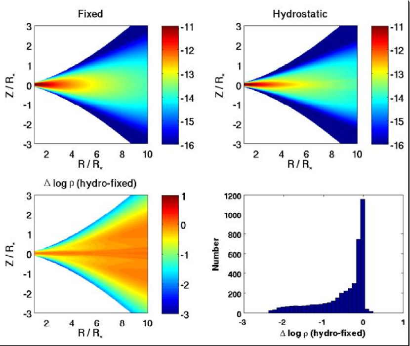
Figure 1: The density structure of a fixed (upper left) and hydrostatic (upper right) disk with $\rho_{o}=5\cdot 10^{-11}\,\rm g\,cm^{-3}$ and $n=3.5$ for the B0 model of Table 1. The lower-left panel shows the differences in $\log(\rho)$ directly, while the lower-right panel gives a histogram of these differences over all 4200 grid points.

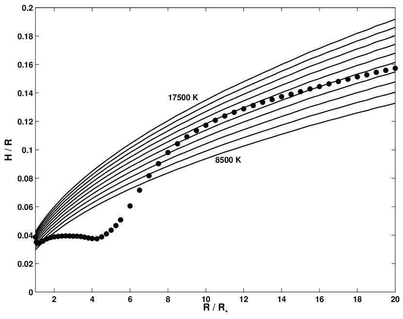
Figure 2: Vertical disk scale height as a function of radial distance for a B0 model with $\rho_{o}=5\,10^{-11}\,\rm g\,cm^{-3}$ and $n=3.5$. The solid lines are scale heights for fixed models (Eqns 1 and 10) with isothermal temperatures ranging from 8500 to $17500\;$K in steps of $1000\;$K (moving upward in the figure). The filled circles are the scale heights of a hydrostatic model of the same $\rho_{o}$ and $n$ found by locating the vertical height at which the density dropped to $1/e$ of its value in the equatorial plane.

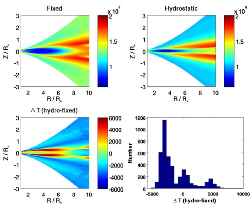
Figure 3: The temperature structure of a fixed (upper left) and hydrostatic (upper right) disk with $\rho_{o}=5\cdot 10^{-11}\,\rm g\,cm^{-3}$ and $n=3.5$ for the B0 model. The lower-left panel shows the temperature differences directly, while the lower-right panel gives a histogram of these differences over all 4200 grid points.

In this comparison, one might question the choice of $T_{o}=13,500\;$K adopted for the fixed model. To address this point, an additional set of fixed calculations was performed by varying $T_{o}$ from $9,500$ to $17,500\;$K with all of the other model parameters held fixed. Figure 4 summarizes these results by giving histograms of the differences in temperature and in the logarithm of the density over the entire grid. As can be seen from Figure 4, the density distribution is best represented by the coolest model, $T_{o}=9,500\;$K. This is not surprising as $\rho_{o}$ is large enough that a cool equatorial region develops with temperatures as low as $8,000\;$K in some regions. Conversely, Figure 4 shows that the temperature is best represented by the hottest model, $T_{o}=17,500\;$K. This result, however, is a bit deceptive. As will be shown in the next section, it is the coolest model which does the best job in reproducing the observables. The large temperature differences in the $T_{o}=9,500\;$K model often result from the misalignment in the height of the cool gas and hot sheaths.

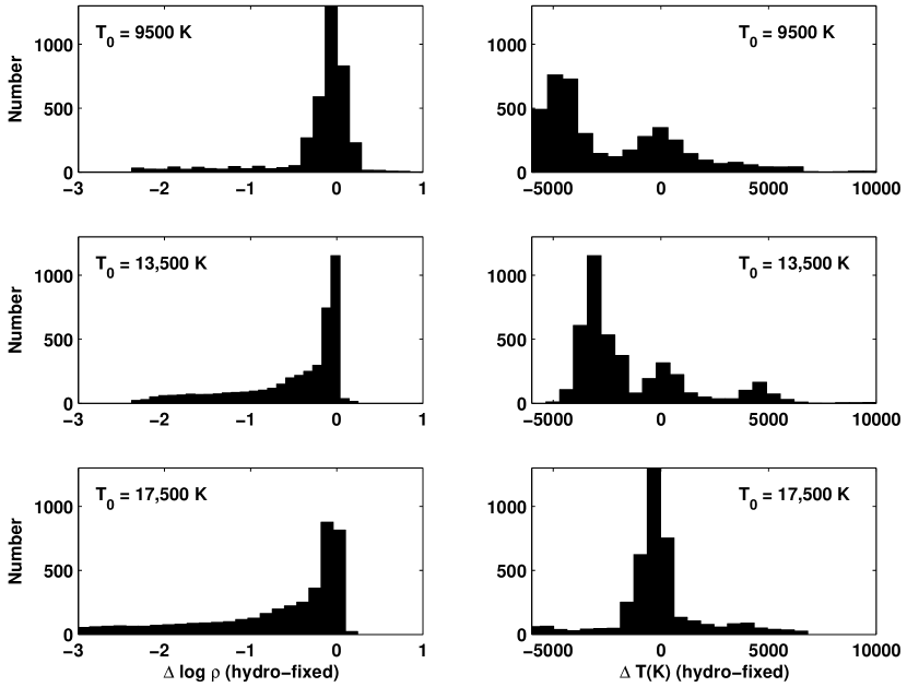
Figure 4: Histograms of the density (left panels) and temperature (right panels) differences between fixed and hydrostatic models for $\rho_{o}=5\cdot 10^{-11}\,\rm g\,cm^{-3}$ and $n=3.5$ for the B0 model. The fixed models assume $T_{o}=9,500\;$K (top row), $13,500\;$K (middle row), and $17,500\;$K (bottom row).

The previous large differences between the fixed and hydrostatic models reflect the poor job the assumption of an isothermal $T_{o}$ does in representing the density structure of a disk that develops a cool equatorial region. Figure 5 illustrates the development of this cool region, for the B0 spectral type, as the overall disk density is increased. Plotted is the density-weighted temperature,

$$<T_{\rm Disk}(R)>\equiv\frac{\int_{0}^{Z_{\rm max}}\rho(R,Z)\,T(R,Z)\,dZ}{\int_{0}^{Z_{\rm max}}\rho(R,Z)\,dZ}\;,$$ (11)

as a function of radial distance for six hydrostatic models with initial densities, $\rho_{o}$, ranging from $5.0\cdot 10^{-13}$ to $1.0\cdot 10^{-10}\;\rm g\,cm^{-3}$. All models assumed $n=3.5$. This figure illustrates that models with $\rho_{o}\lesssim 5.0\cdot 10^{-12}\;\rm g\,cm^{-3}$, do not have an extensive cool, equatorial zone near the star where $T(R,Z)\lesssim 10,000\;$K whereas denser models rapidly develop such a region. This lack of a strong temperature gradient for the less dense models suggests that the isothermal approximation of Eq. 1 is adequate to represent their density structure. This is borne out by Figure 6 which compares the disk temperatures of a low-density ($\rho_{o}=1.0\cdot 10^{-12}\;\rm g\,cm^{-3}$) hydrostatic model with a fixed model computed with the same $\rho_{o}$ and $T_{o}=13,500\;$K. There is little temperature difference between the two models. Figure 7 compares (as histograms) the predicted disk temperatures and densities for three choices of the $T_{o}$ parameter, $9,500$, $13,500$ and $17,500\;$K, with the hydrostatic model. As is clear from this figure, $T_{o}=13,500\;$K does an adequate job of reproducing both the densities and temperatures in the disk.

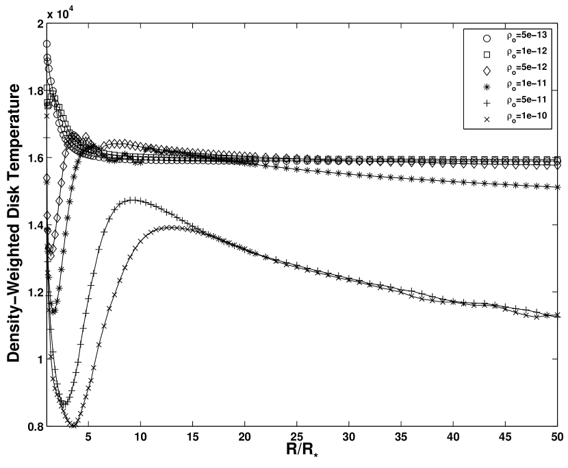
Figure 5: The density-averaged temperature as a function of radial distance for six hydrostatic models corresponding to values of $\rho_{o}$ ranging from $5.0\cdot 10^{-13}\;\rm g\,cm^{-3}$ to $1.0\cdot 10^{-10}\;\rm g\,cm^{-3}$ (see legend) for the B0 model.

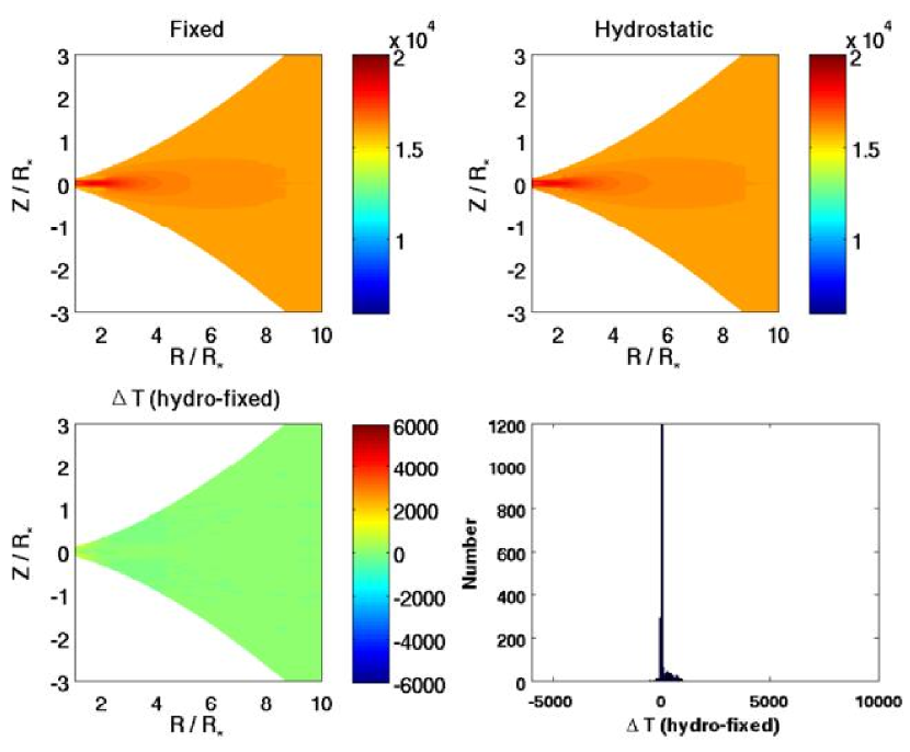
Figure 6: Comparison of the disk temperatures between a fixed (upper left) and hydrostatic (upper right) model with for $\rho_{o}=1\cdot 10^{-12}\,\rm g\,cm^{-3}$ and $n=3.5$ for the B0 model. The fixed model assumes $T_{o}=13,500\;$K.

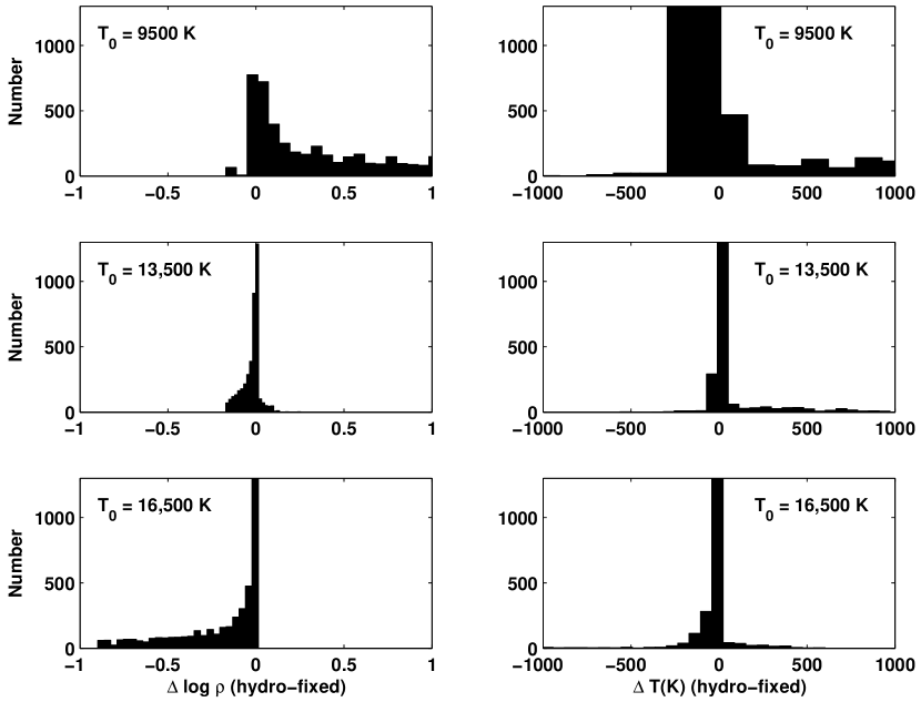
Figure 7: Histograms of the density (left panels) and temperature (right panels) differences between fixed and hydrostatic models for $\rho_{o}=1\cdot 10^{-12}\,\rm g\,cm^{-3}$ and $n=3.5$ for the B0 model. The fixed models assume $T_{o}=9,500\;$K (top row), $13,500\;$K (middle row), and $17,500\;$K (bottom row).

The general conclusion is that the isothermal, fixed $T_{o}$ models are appropriate for low-density disks provided a reasonable choice for $T_{o}$ is made. However, denser disks develop a cool equatorial region and the disk densities and the resultant temperatures cannot be computed assuming a fixed, isothermal density structure. This result is confirmed by similar calculations for the disks surrounding the two later spectral types of Table 1. However, rather than present similar plots and histograms for these models, we will proceed to the next section where a systematic comparison of the predicted density-averaged disk temperatures is made between fixed and hydrostatic models.

4.2 Density-Averaged Disk Temperatures

To further investigate the reliability of the fixed density models, we examine how well they can predict the global, density-weighted, average disk temperature, defined as

$$<T_{\rm Disk}>\equiv\frac{1}{M_{\rm Disk}}\int_{V}\rho\,T\,dV\;.$$ (12)

Here $M_{\rm Disk}$ is the total mass of the disk, and the integral is over the total volume of the disk.

Equation 12 was computed for 9 central stars, ranging in $T_{\rm eff}$ from $13,800\;$K to $30,000\;$K in order to cover the full range of Be star spectral types. For each central star, 14 disk models were computed for different choices of the base disk density, $\rho_{o}$, covering the range $\rho_{o}=2.5\cdot 10^{-13}\;\rm g\,cm^{-3}$ to $5.0\cdot 10^{-10}\;\rm g\,cm^{-3}$. All models assumed an $n=3.5$ radial power-law index. In total, 126 hydrostatic disk models were computed. Figure 8 shows the results with the density-weighted, disk temperature expressed as a fraction of the stellar $T_{\rm eff}$. The (unweighted) average ratio at each $T_{\rm eff}$ (shown in the figure by the filled squares) is well-fit by the quadratic relation

$$\frac{<T_{\rm Disk}>}{T_{\rm eff}}=0.096\,T^{2}_{4}-0.448\,T_{4}+1.098\;,$$ (13)

where $T_{4}$ is the stellar effective temperature in units of $10^{4}\;$K. Over the $T_{\rm eff}$ range of the Be stars, the average ratio ranges between 0.55 and 0.65, suggesting some validity to the often-used approximation that a good estimate for an (isothermal) disk temperature is a constant fraction of the stellar $T_{\rm eff}$ (for example, Waters et al. (1987) adopted $<T_{\rm Disk}>=0.8\,T_{\rm eff}$). Similar ratios are found throughout the literature, including some based on sophisticated modeling, such as that of Carciofi & Bjorkman (2006) who found a ratio of 0.6 for moderate density disks surrounding a B3 IV star. The current work finds that $<T_{\rm Disk}>/T_{\rm eff}\approx 0.6$ is a reasonable fit to the average trend over the entire range of Be stars, with the quadratic fit of Eqn (13) representing a marginal improvement. However, the current work also makes clear that at each individual $T_{\rm eff}$, the scatter about this average is large and depends in a systematic way on the disk density $\rho_{o}$. Increasing the overall density drives the density-weighted temperatures to lower values due to the development of the cool equatorial zone noted in Figure 5. As shown in Figure 8, ratios as low as 0.45 can be predicted for dense disks, and ratios as high as 0.7 for rarefied disks.

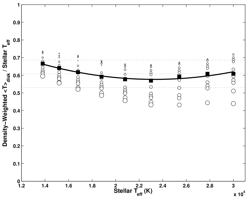
Figure 8: Density-weighted disk temperature (Equation 12) as a function of the central star’s $T_{\rm eff}$. At each $T_{\rm eff}$, the open circles represent disks with different base densities, $\rho_{o}$, with the size of the symbol signifying the size of $\rho_{o}$. The smallest circles correspond to $\rho_{o}=2.5\cdot 10^{-13}\;\rm g\,cm^{-3}$ and the largest circles, to $\rho_{o}=5.0\cdot 10^{-10}\;\rm g\,cm^{-3}$. The filled squares are the (unweighted) average temperatures, and the solid line is the quadratic fit given by Equation (13).

To examine the accuracy of the fixed models in predicting the density-weighted disk temperature over a wide range of central effective temperatures and disk densities, the 126 models were rerun but this time as fixed density models with $T_{o}$ (see Equation 7 and discussion) chosen to be equal to the $<T_{\rm Disk}>$ predicted by the corresponding hydrostatic model. Figure 9 compares the $<T_{\rm Disk}>$ predicted by the fixed models to the hydrostatic results. As can be seen from the figure, the fixed models with an appropriately chosen $T_{o}$ can reproduce the $<T_{\rm Disk}>$ of the hydrostatic models to within $\pm 500\;$K over a wide range of $T_{\rm eff}$ and $\rho_{o}$. This is particularly true for the models with low values for $\rho_{o}$, which scatter well within $\pm 250\;$K. However, larger deviations occur for the denser disks and, for $T_{\rm eff}>18,000\;$K, the fixed models for the largest densities all predict hotter $<T_{\rm Disk}>$ values by up to $1500\;$K.

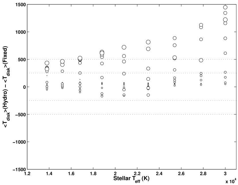
Figure 9: Difference between the density-weighted disk temperature predicted by the fixed and hydrostatic models. For the fixed models, the $T_{o}$ parameter was chosen to be the hydrostatic prediction for $<T_{\rm Disk}>$. As in Figure (8), the open symbols represent the different base densities chosen for each disk.

Despite this reasonable agreement, it is very important to next see if fixed models can be used to successfully predict more readily observed diagnostics such as H$\alpha$ line profiles and infrared excesses.

4.3 Observational Diagnostics

To demonstrate more direct observational consequences of consistent vertical hydrostatic equilibrium, we considered a disk with a density of $\rho_{o}=5.0\cdot 10^{-11}\;\rm g\,cm^{-3}$ and $n=3.5$. As noted in Section 4.1, this density is large enough that a cool equatorial region forms close to the star where the vertical temperature distribution is far from isothermal. Radiative equilibrium solutions were found for the fixed density structure of Eq. 1 for several values of the $T_{o}$ parameter. Observable quantities were computed for each of these fixed models to see if any could reproduce the observational predictions of the hydrostatic disk with the same $\rho_{o}$ and $n$. This process was repeated for each of the three stars given in Table 1 which correspond spectral types B0, B2, and B5.

The first observational diagnostic considered is the predicted H$\alpha$ line profile corresponding to each model. The H$\alpha$ line profile was obtained by solving the transfer equation using the hydrogen level populations predicted by bedisk. In all cases, a viewing angle of $i=35\,$ degrees was chosen (where $i=0$ corresponds to a pole-on star) and the equatorial velocity was set to $325\;\rm km\,s^{-1}$. This results in a projected stellar rotation velocity of $v\,\sin\,i=186\;\rm km\,s^{-1}$. An equatorial velocity of $325\;\rm km\,s^{-1}$ is approximately 70% of the critical rotation velocities given the parameters of Table 1. Pure Keplerian rotation, with zero outflow velocity, was assumed for the disk.

To represent the stellar disk, an LTE, photospheric, H$\alpha$ line profile was used corresponding to the $T_{\rm eff}$ and $\log(g)$ of Table 1, The profile for each element of the stellar surface was shifted by its projected radial velocity, resulting in a rotationally broadened photospheric profile. For the calculation of the H$\alpha$ emissivity and opacity in the disk, the Stark profiles of Barklem & Piskunov (2003) were used.

Figure 10 shows the resultant H$\alpha$ line profiles predicted by the hydrostatic and fixed models for each of the three spectral types considered. The fourth panel shows the variation with $T_{o}$ of the total H$\alpha$ equivalent width of the fixed models. The equivalent widths of the consistent hydrostatic models are also shown. The H$\alpha$ equivalent width increases with $T_{o}$ for the fixed models and the increase is $\approx\,30$% for a factor of two increase in $T_{o}$. Typically, the fixed model with (nearly) the lowest value of $T_{o}$ is most successful in matching the hydrostatic prediction. This again reflects the influence of the cool equatorial region that develops in the higher-density disks. The H$\alpha$ emissivity is controlled mainly by the high temperature “sheaths” above and below the equatorial plane in the inner disk. The lower $T_{o}$ values better represent the actual inner disk scale heights thus placing the hot sheaths closer the location predicted by the hydrostatic models (see Figure 3).

Another observational diagnostic is the infrared excess predicted by the models. Infrared excesses (expressed in magnitudes), relative to the underlying photospheric contribution, are shown in Figure 11. Again, the excess is found by solving the transfer equation along a series of rays threading the disk system. To represent the star, an LTE, line-blanketed stellar atmosphere was used corresponding to the parameters listed in Table 1. Solutions were obtained at three wavelengths in the near-infrared, 2, 5, and 15$\;\mu$m. The predicted IR excess for a series of fixed disk models with varying $T_{o}$ are shown in Figure 11. Also shown in the figure are the predictions of the hydrostatic models with the same $\rho_{o}$ and $n$ for each spectral type. For the earlier spectral types, the differences are generally small, within a few tenths of a magnitude, for plausible choices of $T_{o}$. However, larger differences are predicted for the latest spectral type considered, B5. Close inspection of this figure also shows that there is, in general, no single choice for $T_{o}$ that will reproduce the IR excess at the three wavelengths considered. Typically a higher $T_{o}$ is required to match the excess at a shorter wavelength; this effect is particularly clear in the B5 model where the magnitude differences are largest.

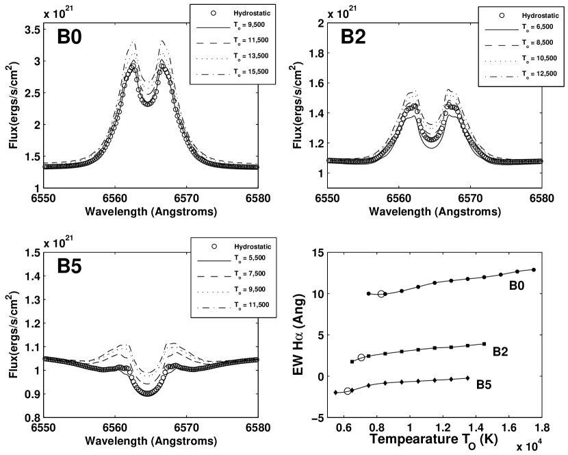
Figure 10: Predicted H$\alpha$ line profiles for hydrostatic models and fixed models (assuming various $T_{o}$) for three stellar spectral types (upper panels and lower left panel). The variation of the H$\alpha$ equivalent width (in Å) for these stars as a function of $T_{o}$ for the fixed models is also shown in the lower right panel. The equivalent width predicted by the hydrostatic model associated with these stars is shown as an open circle.

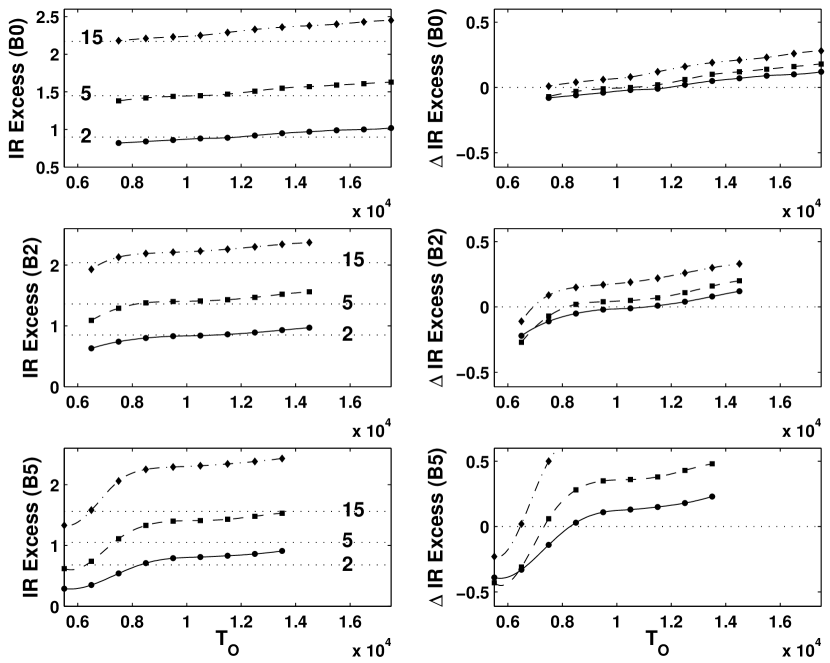
Figure 11: Predicted IR excess for a series of fixed disk models computed by varying $T_{o}$ for three stellar spectral types. Absolute IR excesses are shown on the panels on the left. The line styles and symbols correspond to wavelengths of 2$\,\mu$m (solid line, circles), 5$\,\mu$m (dashed line, squares), and 15$\,\mu$m (dash-dot line, diamonds). The predictions of the hydrostatic models are shown as a dotted line with the wavelength in $\mu$m as indicated. The differences in the IR excess, fixed minus hydrostatic, are shown in the right-hand panel. The line styles have the same interpretation except that the dotted line in each shows the zero magnitude difference for reference.

5 Conclusions

In this work, we have compared predicted disk temperatures, densities, H$\alpha$ line profiles and equivalent widths, and near-IR excesses between a set of Be disk models computed in consistent radiative and vertical hydrostatic equilibrium and a set of corresponding radiative equilibrium models that assumed a fixed density structure. Large differences between the predicted temperatures and densities can occur between the hydrostatic and fixed models when the density is large enough that the disk develops a cool equatorial region close to the star. In this case, there seems to be no choice for the single, isothermal temperature $T_{o}$ that characterizes the fixed density structure that will yield a model matching the observational signatures of a consistent model.

These conclusions are particularly important given the way such sets of Be disk models are used to compare to observations and extract disk parameters. Typically, a grid of models is computed for a wide range of $\rho_{o}$ with a fixed density structure parametrized by a single temperature $T_{o}$ (see for example Sigut & Jones, 2007). This grid is then used to compared to observations of, say, H$\alpha$ line profiles or IR excesses to select the most appropriate disk parameters. As shown in this work, such a grid will contain a systematic error in the predictions for high $\rho_{o}$ where a cool equatorial region in the disk develops; such models are poorly approximated by disks with a density structure fixed a priori. To extract the “true” distribution of disk parameters, within the context of a thin disk in vertical hydrostatic equilibrium, a grid which consistently enforces both radiative and vertical hydrostatic equilibrium should be employed.

References

- Barklem & Piskunov (2003) Barklem, P. S., & Piskunov, N. E. 2000 in Modelling of Stellar Atmospheres, IAU Symposium 210, N. E. Piskunov, W. W. Weiss, & D. F. Gray eds., p.E28
- Carciofi & Bjorkman (2006) Carciofi, A. C., & Bjorkman, J. E. 2005, ApJ, 639, 1081
- Dougherty et al. (1994) Dougherty, S. M., Waters, L. B. F. M., Burki, G., Coté, J., Cramer, N., van Kerkwijk, M. H., & Taylor, A. R. 1994, A&A, 290, 609
- Jones et al. (2009) Jones, C. E., Molak, A., Sigut, T. A. A., de Kota, A., Lenorzer, A., & Popa, S. C. 2009, MNRAS, 392, 383
- Jones et al. (2008) Jones, C. E., Tycner, C., Sigut, T. A. A., Benson, J. A., & Hutter, D. J. 2008, ApJ, 687, 598
- Jones, Sigut & Porter (2007) Jones, C. E., Sigut, T. A. A., & Porter, J. M. 2007, MNRAS, 386, 1922
- Jones, Sigut & Marlborough (2004) Jones, C. E., Sigut, T. A. A., & Marlborough, J. M. 2004, MNRAS, 352, 841
- Osterbrock (1989) Osterbrock, D. E. 1989, Astrophysics of Gaseous Nebulae and Active Galactic Nuclei (Mill Valley: Univ. Sci. Books)
- Poeckert & Marlborough (1978) Poeckert, R., & Marlborough, J. M. 1978, ApJ, 220, 940, PM
- Porter (1999) Porter, J. M. 1999, A&A, 348, 512
- Porter & Rivinus (2003) Porter, J. M., & Rivinius, T. 2003, PASP, 115, 1153
- Quirrenbach et al. (1993) Quirrenbach, A., Hummel, C. A., Buscher, D. F., Armstrong, J. T., Mozurkewich, D., & Elias, N. M. II 1993, ApJ, 416, L25
- Sigut & Jones (2007) Sigut, T.A.A., & Jones, C. E. 2007, ApJ, 668, 481
- Tycner et al. (2008) Tycner, C., Jones, C. E., Sigut, T. A. A., Schmitt, H. R., Benson, J. A., Hutter, R. T., & Zavala, R. T. 2008, ApJ, 689, 461
- Tycner et al. (2005) Tycner, Christopher, Lester, John B., Hajian, Arsen R., Armstrong, J. T., Benson, J. A., Gilbreath, G. C., Hutter, D. J., Pauls, T. A., & White N. M 2005, ApJ, 624, 359
- Tycner et al. (2006) Tycner, Christopher, Gilbreath, G. C., Zavala, R. T., Armstrong, J. T., Benson, J. A., Hajian, Arsen R., Hutter, D. J., Jones, C. E., Pauls, T. A., & White, N. M. 2006, AJ, 131, 2710
- Waters (1986) Waters, L. B. F. M. 1986 A&A, 162, 121
- Waters et al. (1987) Waters, L. B. F. M., Cote, J., & Lamers, H. J. G. L. M. 1987, A&A, 185, 206
- Waters & Marlborough (1992) Waters, L. B. F. M., & Marlborough, J. M. 1992 A&A256, 195
- Wood et al. (1997) Wood K., Bjorkman K. S., & Bjorkman J. E. 1997, ApJ, 477, 926