The nature of the line profile variability in the spectrum of the massive binary HD 152219

Abstract

Context. HD 152219 is a massive binary system with O9.5 III + B1-2 V/III components and a short orbital period of 4.2 d. Its primary component further displays clear line profile variability (LPV). The primary component being located within the pulsational instability domain predicted for high-luminosity stars, we previously suggested that the observed LPV could be associated with non-radial pulsations.

Aims. The aim of the present work is to determine the nature of the observed LPV in the spectrum of the primary component of HD 152219.

Methods. During a 4-night FEROS monitoring campaign, we collected a new set of 134 high signal-to-noise spectra. These new observations were then used to re-investigate the variability of different line profiles in the spectrum of HD 152219.

Results. Based on the present analysis, we discard the non-radial pulsations and point out the Rossiter-McLaughlin effect as the cause of the LPV in HD 152219. The upper limit on the amplitude of possible weak pulsations is set at a few parts per thousand of the continuum level.

Conclusions.

1 Introduction

With only a few objects known to present pulsations, asteroseismology of massive stars remains essentially a terra incognita. This partly results from the lack of dedicated observational studies and the difficulty of disentangling possible pulsations from wind effects or co-rotating structures. Among the known O-type pulsators, $ζ$ Oph (O9 V) is the best studied object, with 19 frequencies identified either photometrically or spectroscopically and corresponding both to radial and non-radial pulsations (Walker et al. 2005, and reference therein). HD 93521 is an isolated O9.5 Vp star exhibiting non-radial pulsations (NRPs) with periods of 1.8h and 2.9h, corresponding to harmonic degrees $l$ of 9 and 5 respectively (Rauw et al. 2008; Howarth et al. 1998). Other candidates that could harbor NRPs are $ζ$ Pup (Reid & Howarth 1996), $ξ$~Per and $λ$ Cep (de Jong et al. 1999), and HD 152249 (Gosset et al. 2008). Additionally, Fullerton et al. (1991) suggested that the O7 II star HD 34656 shows radial pulsations, possibly revealing the radial fundamental mode.

HD 152219 is an O9 III + B1-2 III/V short period binary ($P\sim 4.2$ d) in the core of the NGC 6231 cluster. In Sana et al. (2006, Paper I), we showed that the primary component displays clear line profile variability (LPV). With $\log T_{\mathrm{eff}}=4.50$ and $\log L/L_{\odot}=5.07$, the primary star lies on the prolongation of the $\beta$ Cep instability strip (e.g., Pamyatnykh 1999; Miglio et al. 2007), within the domain of instability predicted by Pamyatnykh (1999) for high-luminosity stars.

In the present paper, we report on a 4-night intensive monitoring campaign of the object, that aimed at determining the nature of the observed LPVs. In Paper I, we focused on the He ii$\lambda$4686 line as it is the only well isolated, strong primary line that is uncontaminated by the secondary signature or by neighbouring lines. This strategy not only renders the analysis more straightforward, but it has the further advantage of avoiding any poorly quantified effects that can hamper spectral disentangling methods in the presence of varying spectral signatures (see e.g., Linder et al. 2008). In the present paper, we analyze a larger subset of lines: H$\beta$, He i$\lambda\lambda$4712, 4921, 5875, 6678 and He ii$\lambda$4686.

Table 1: Synthetic view of the June 2006 FEROS campaign. The first column indicates the night number with respect to the beginning of the campaign. The second and third columns yield the heliocentric Julian date (in format HJD$-$2 450 000) and phase interval ranges covered. The last column lists the number $n$ of spectra obtained each night.

#	HJD range	$\phi_{\lambda 4686}$	$n$
1	3911.50709–3911.86854	0.754–0.839	19
2	3912.47729–3912.87965	0.983–0.078	32
3	3913.47072–3913.88523	0.217–0.315	49
4	3914.48017–3914.87588	0.455–0.548	34

Table 2: Sample of the journal of the spectroscopic observations of HD 152219. ‘HJD’ gives heliocentric Julian date (HJD$-$2 450 000) at mid-exposure. $\phi_{\lambda 4686}$ indicates the corresponding phase according to the new He ii$\lambda$4686 ephemeris of Table 3. $RV_{1}$ gives the primary radial velocity as measured on the He ii$\lambda$4686 line. ‘Exp’ lists the exposure time (in seconds) while ‘SNR’ indicates the measured signal-to-noise ratio in the range 4740–4750Å. The full table is available at the CDS.

HJD	$\phi_{\lambda 4686}$	$RV_{1}$	Exp	SNR
3860.81531	0.804	20.15	900	320
3861.66960	0.005	$-$133.85	900	323
3861.92118	0.064	$-$149.33	900	361
3862.65506	0.237	$-$69.29	900	284
3862.90246	0.296	$-$29.43	900	356
3863.64302	0.470	74.92	900	294
3863.88654	0.528	90.92	900	380
3864.65014	0.708	67.76	720	310
3864.86446	0.758	42.87	600	334
3911.50709	0.758	38.58	1200	142
3911.52338	0.762	38.77	1500	276
3911.55914	0.771	29.30	900	215
3911.57020	0.773	28.47	900	275
3911.58127	0.776	27.06	900	223
3911.61757	0.784	17.72	1200	194
3911.63210	0.788	15.42	1200	229
3911.64664	0.791	15.23	1200	213
3911.66996	0.797	14.08	1200	306
3911.68451	0.800	13.18	1200	325
3911.69905	0.804	14.59	1200	368
3911.71393	0.807	14.65	1200	276
3911.72847	0.811	14.59	1200	285
3911.76994	0.820	14.52	1200	302
3911.79196	0.826	12.80	1020	249

2 Observations and data reduction

During four consecutive nights in June 2006, we intensively monitored HD 152219, using the FEROS echelle spectrograph mounted on the ESO/MPG 2.2m telescope at La Silla (Chile). The detector was a 2k $\times$ 4k EEV CCD with a pixel size of 15$\mu$m $\times$ 15$\mu$m. The spectral resolving power of FEROS is 48 000. The atmospheric dispersion corrector (ADC) was used to maximize the throughput at high airmass (up to $z<3$), but it was also used at low airmass to preserve the homogeneity of the data set. The exposure time was varied between about 300 and 1200 sec in order to match the observing conditions (airmass, atmosphere transparency, seeing) but also to cover various time ranges. The campaign yielded a total of 134 spectra. The resulting signal-to-noise ratios (SNR), as measured on the reduced 1D spectra in the continuum region 4740–4750Å, are all above 200, but for 10 spectra. On average, the SNR is close to 300. Table 1 provides a synthetic view of the campaign while Table 2 presents the journal of the observations. The full table is available at the CDS and, beyond the sample data displayed here, the table further contains all the RV measurements performed on the various lines studied in this paper

As a complement to the June 2006 campaign, nine FEROS spectra were obtained during five consecutive nights in May 2006 in order to improve the accuracy of the ephemeris. The typical exposure time was 900 sec and the obtained SNR about 300 as seen from Table 2.

The data reduction was performed using a modified FEROS pipeline working under the MIDAS environment. Beyond the modifications already described in Paper I, several new features were implemented. We used a 2D fit of the order position for improved stability. We also used the wavelength calibration frames obtained with the ‘new’ ThArNe calibration lamp (see e.g., Pritchard 2005). The latter however heavily saturates in the red, even on the shortest exposures provided by the calibration plan. At the time of our observations, the daily FEROS wavelength calibrations consisted of 3 series of two exposures with increasing exposure times of 3s, 15s and 30s, a scheme that is repeated at the begining and at the end of the night. To optimize the wavelength calibration, we computed a master calibration frame for each exposure time, by summing the frames with identical exposure times. We then extracted the ThArNe calibration spectra separately for each master frame. We finally used the detected lines from the 3s/15s/30s master frames to respectively calibrate the orders 30–39/10–29/1–9. The saturated lines or the lines outside the linearity range of the detector were rejected from the fit and the detection threshold was optimized for each order. Finally, a 2-iteration 3-sigma clipping method was used to discard the very few remaining discordant lines (mostly because of artifacts related to poorly corrected bad column effects). The obtained wavelength calibration residuals were all in the range 2.7-2.9 mÅ.

Table 3: Orbital solutions deduced from different lines (Col. 1). The usual notations for the orbital elements have been used. Quoted uncertainties are the 1-$\sigma$ error bars.

Line	$P$	$e$	$\omega$	$K_{1}$	$\gamma_{1}$	r.m.s.
	(d)		(∘)	(km s-1)	(km s-1)	(km s-1)
H$\beta$	4.24021	0.058 $\pm$ 0.006	140 $\pm$ 5	117.0 $\pm$ 0.5	$-29.6\pm$ 0.6	4.9
He ii $\lambda$4686	4.24029	0.085 $\pm$ 0.003	153 $\pm$ 1	124.4 $\pm$ 0.2	$-17.3\pm$ 0.3	2.0
He i $\lambda$4922	4.24023	0.057 $\pm$ 0.006	148 $\pm$ 4	107.7 $\pm$ 0.4	$-17.9\pm$ 0.5	3.8
He i $\lambda$5015	4.24015	0.059 $\pm$ 0.006	150 $\pm$ 4	112.1 $\pm$ 0.4	$-22.2\pm$ 0.6	4.0
He i $\lambda$5876	4.24021	0.069 $\pm$ 0.004	151 $\pm$ 2	115.9 $\pm$ 0.3	$-22.4\pm$ 0.4	2.9
He i $\lambda$6678	4.24022	0.061 $\pm$ 0.005	151 $\pm$ 3	114.4 $\pm$ 0.4	$-14.7\pm$ 0.5	3.2

Figure 1: Upper panel: HD 152219 RV-curve corresponding to the updated He ii$\lambda$4686 orbital solution of Table 3. The dashed line indicates the systemic velocity. Lower panel: Residuals of the fit, in the sense data minus model. The dotted lines indicate the $\pm$ 1-$\sigma$ domain around the zero point of the solution (dashed line).

3 Updated orbital solutions

In Paper I, we showed that radial velocity (RV) solutions derived from different spectral lines could show significant systematic differences. In particular the semi-amplitude of the RV curves derived from different lines could differ by up to 10 km s^-1. As a necessary step in the LPV analysis (see Sect. 4) is to correct the observed spectra for the primary motion, we first computed updated orbital solutions for each of the considered spectral lines.

As for the data of Paper I, we measured the Doppler shifts by fitting one or two Gaussians to the line profiles, depending whether the SB2 signature was visible or not. The RVs were then computed adopting the same rest wavelengths as in Paper I (Conti et al. 1977; Underhill 1994). While other authors have showed that more accurate RVs can be obtained by using a cross-correlation technique (e.g., Rauw et al. 2001), the more straightforward Gaussian-fitting method still allows us to reach a RV accuracy of a few km s^-1 or better, which is sufficient for our purpose. Beyond the present data set, we also used the data of Paper I to obtained the RVs of several lines that were not studied in Paper I but that are analyzed here.

As our aim is to correct for the primary orbital motion, we exclusively focused on the primary orbital solution. Combining the current data with the data from Paper I, we computed new orbital solutions for each line, using the Liège Orbital Solution Package (LOSP, Sana & Gosset 2009). The uncertainties quoted in Table 3 were computed using the observed dispersion of a set of 1000 simulated solutions through the Monte-Carlo simulation module of the package. The new orbital solutions are compatible, within the uncertainties, with those quoted in Paper I. As discussed in Sect. 4, RV measurements performed in the phase interval $\phi_{\lambda 4686}=0.71-0.95$ are not representative of the motion of the star mass center and, indeed, those points show larger residuals. In a second step, we thus recomputed the orbital solutions excluding observations obtained during that phase range. This significantly improved the residuals of the fit. Table 3 provides the updated orbital solutions for the different lines. The main noticeable difference with Paper I is a reduced eccentricity. While the new values remain marginally within the 3-$\sigma$ errors bars of Paper I, the observed differences can also be due to a slow apsidal motion as suggested by Mayer et al. (2008).

As the He ii$\lambda$4686 line is the only line in our sample that is uncontaminated by the secondary signature, and as the He ii$\lambda$4686 solution shows the lowest residuals, we will adopt the He ii$\lambda$4686 ephemeris in the rest of this paper. In the following, the periastron passage of the He ii$\lambda$4686 solution, at $T_{0}=2\,453\,997.338$ (HJD), is adopted as phase zero: $\phi_{\lambda 4686}=0.0$. The He ii$\lambda$4686 RV-curve is displayed in Fig. 1.

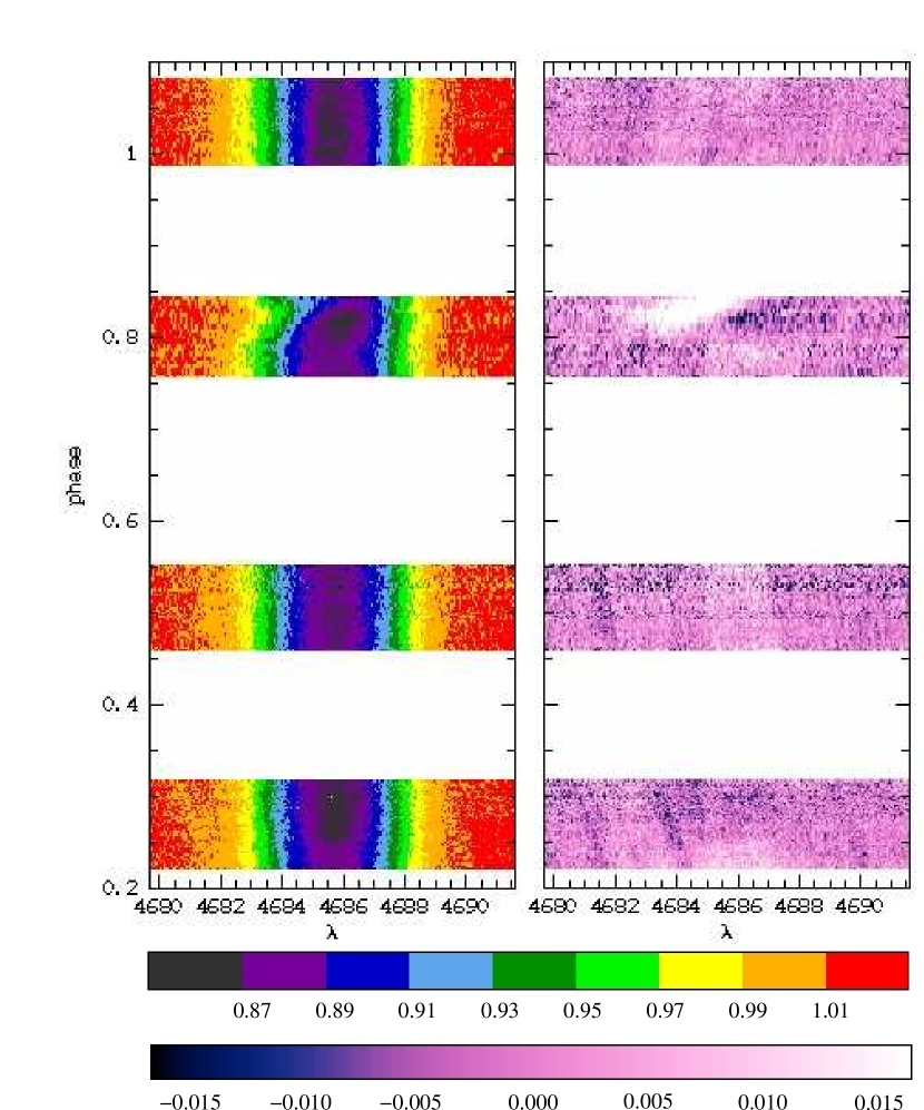
Figure 2: Left panel: Color-coded image of the evolution of the He ii$\lambda$4686 line profile with the phase. Spectra are displayed in the reference frame of the primary. Right panel: same as left panel for the difference spectra, i.e. the spectra minus the median spectrum computed over all non-eclipse phases. Color scales for both panels are indicated at the bottom of the image.

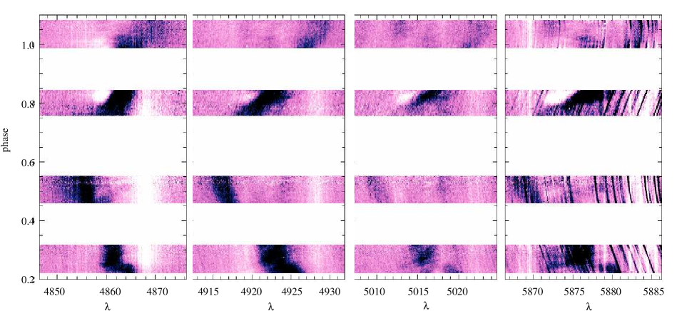
Figure 3: Evolution of the difference spectra for the H$\beta$ and He i$\lambda$4922, 5015, 5876 lines. The color scale is identical to the one of Fig. 2 (right panel).

4 Line profile analysis

Using the updated orbital solutions, we corrected the spectra for the primary motion. As an example, Fig. 2 (left panel) shows the evolution of the He ii$\lambda$4686 line profile in the primary reference frame. It clearly illustrates that the main LPV is observed at $\phi_{\lambda 4686}\sim 0.79-0.91$, which corresponds to the time of the primary eclipse, when the companion is passing in front of the primary (an effect known as the Rossiter-McLaughlin effect). Additionally, one can also see a change of the intensity of the He ii$\lambda$4686 line during the secondary eclipse ($\phi_{\lambda 4686}\sim 0.23-0.37$), resulting from the changing dilution of the line by the varying continuum. However, there seems to be little or no profile variations outside those phase intervals.

To increase the dynamics of the image, we computed the median spectrum outside eclipse phases. The median spectrum was subsequently subtracted from all our spectra, yielding ‘difference spectra’. Fig. 2 (right panel) shows the evolution of He ii$\lambda$4686 difference spectra with phase. Clearly, no further LPV pattern can been seen at the $\approx 0.005$ fraction of the continuum level.

Similarly, Fig. 3 shows the evolution, along with the phase, of the H$\beta$ and He i$\lambda\lambda$4922, 5015, 5876 difference spectra. The primary profile during nights #1 and #3 ($\phi_{\lambda 4686}\sim 0.8$ and 0.25) are clearly blended with the secondary signature. During nights #2 and #4 ($\phi_{\lambda 4686}\sim 1.05$ and 0.5), the separation between the two components is large enough, so that the primary profile can be searched for NRP signatures. As for the He ii$\lambda$4686 line however, no profile variations can be detected beyond the eclipse effects.

Figure 4: Averaged line profile (upper panels) and square root of the TVS (lower panels) for three different lines. On the upper panels, the dotted lines show the continuum level while the dashed lines indicate the primary velocity frame. On the lower panels, the dotted lines indicate the variability threshold corresponding to a significance level of 0.001.

To quantitatively verify that no significant LPV are present, we computed the Time Variance Spectrum (TVS, Fullerton et al. 1996) using only spectra obtained during night #2 and #4, thus outside the eclipse phases. While we followed the original idea of Fullerton et al. (1996), we have weighted each pixel in the TVS by its standard deviation. Fig. 4 shows the averaged (outside eclipse) profiles of the He ii $\lambda$4686 and He i$\lambda\lambda$4922, 5015 lines and the corresponding TVS spectra. Using the formalism proposed by Fullerton et al. (1996), we tested our data against the null hypothesis ‘not variable’, adopting a significance level of 0.001. Beside some variations in the wings of the He i lines due to the displacement of the secondary lines in the primary reference frame, it is clear from Fig. 4 that the null hypothesis cannot be rejected. As a consequence, we consider the null hypothesis to be very likely and we conclude that no significant variability is seen in the primary line profile (except for the eclipse effects).

We alse performed a similar TVS analysis on the H$\beta$ and He i$\lambda\lambda$5876, 6678 lines, but these lines turned out to be inadequate for our purposes. The He i$\lambda\lambda$5876 line profile is polluted by atmospheric H₂O lines that varies due to the different amount of water vapor along the observing run and to the large airmass spaned by the observations. The He i$\lambda\lambda$6678 blend is located in a telluric-free window of the red spectrum. Unfortunately it is partly affected by residual fringing that is not fully corrected by the flat-fielding. Finally, the H$\beta$ secondary line is so broad that, even at maximum separation, it still strongly contaminates the primary line profile. Despite the fact that the TVS is not applicable, inspection of Fig. 3 still reveals that no clear NRP signature can be seen in those lines.

While we now concludes that NRPs remain undetected in our observations, the high quality of the current data set allows us to put strong constraints on the upper limit of potential low-amplitude non-radial pulsations (NRPs), by using the square-root of the time variance. From Fig. 4, the noise level across the line profile is about 4$\times 10^{-3}$ of the continuum level. As shown in Paper I, the primary companion is expected to contribute to about 91% of the continnum level. Assuming that the secondary is not contributing at all to the noise, we can set up the detection limit at a fraction of 0.005 of the primary continuum.

Table 4: Physical parameters of the known and suspected non-radial pulsators.

Object	Sp.Type	$\log\frac{L}{L_{\odot}}$	$\log T_{\mathrm{eff}}$	$\log g$	Statusa
			(K)	(cm s${}^{-2})$
HD 93521	O9.5V	4.62	4.48	3.92	C
$\zeta$ Oph	O9V	4.72	4.50	3.92	C
HD 152219b	O9.5III	5.21	4.50	3.51	N
$\xi$ Per	O7.5III	5.36	4.52	3.59	C
HD 152249	O9I	5.54	4.47	3.23	S
$\lambda$ Cep	O6I	5.78	4.55	3.48	C
$\zeta$ Pup	O5I	5.87	4.59	3.57	S

5 Discussion

The analysis of a high-quality times series of the profiles of H$\beta$, of He ii$\lambda$4686 and of various He i lines in the HD 152219 spectrum failed to reveal any significant LPV beside the Rossiter-McLaughlin effect. The data displays a SNR close to 300 on average and have allowed us to place an upper limit on the variability level (and thus on the amplitude of possible NRPs in HD 152219) as low as a few parts per thousand of the continuum level.

Table 4 lists some of the known and suspected non-radial pulsators among O-type stars. The quoted physical properties are taken from Martins et al. (2005), based on the spectral type of the objects. Along the luminosity axis, HD 152219 is roughly located between $\zeta$ Oph on one side and $\xi$ Per and HD 152249 on the other, in a yet poorly mapped region of the Hertzsprung-Russell diagram (HRD). HD 152219 thus lies roughly in-between the confirmed main sequence non-radial pulsators and the suspected brighter giant and supergiant ones. Yet, this luminosity sequence does not correlate well with the observations of NRPs. This might thus suggest the existence of two different regimes for the instability domain for massive stars, separated by a region where the NRPs are inhibited or have a much smaller amplitude. Results from on-going theoretical work are eagerly awaited, to revise the expected instability domain of the high-mass stars and to identify the key parameters that govern the pulsational processes in massive stars.

Because very few high quality monitorings of massive stars exist so far, the upper limit derived in the present paper can further be used to test asteroseismology models and to help to accurately constrain the exact location of the high-luminosity end of the instability strip in the Hertzsprung-Russell diagram.