Dynamic effective mass of granular media and
the attenuation of structure-borne sound

Abstract

We report a theoretical and experimental investigation into the fundamental physics of why loose granular media are effective deadeners of structure-borne sound. Here we demonstrate that a measurement of the effective mass, $\tilde{M}(\omega)$, of the granular medium is a sensitive and direct way to answer the question: What is the specific mechanism whereby acoustic energy is transformed into heat? Specifically, we apply this understanding to the case of the flexural resonances of a rectangular bar with a grain-filled cavity within it. The pore space in the granular medium is air of varying humidity. The dominant features of $\tilde{M}(\omega)$ are a sharp resonance and a broad background, which we analyze within the context of simple models. We find that: a) On a fundamental level, dampening of acoustic modes is dominated by adsorbed films of water at grain-grain contacts, not by global viscous dampening or by attenuation within the grains. b) These systems may be understood, qualitatively, in terms of a height-dependent and diameter-dependent effective sound speed [$\sim 100-300\;(m\cdot s^{-1})$] and an effective viscosity [$\sim 5\times 10^{4}$ Poise]. c) There is an acoustic Janssen effect in the sense that, at any frequency, and depending on the method of sample preparation, approximately one-half of the effective mass is borne by the side walls of the cavity and one-half by the bottom. d) There is a monotonically increasing effect of humidity on the dampening of the fundamental resonance within the granular medium which translates to a non-monotonic, but predictable, variation of dampening within the grain-loaded bar. PACS Numbers: 45.70.-n, 46.40.-f, 81.05.Rm

I Introduction

Loose grains, made of a variety of different materials, dampen structure-borne acoustic signals very efficiently when they partially fill cavities within the structure itself Kuhl ; cremer ; Bourinet1 . For this reason, there is a practical motivation to develop an effective method to optimize the dampening of unwanted structure-borne acoustic signals. The fundamental origins of the dissipation mechanisms in granular materials are still unknown, however, making it difficult to optimize the effect. Partly, this is because, until now, it has not been possible to study the relevant properties of the granular medium directly, independent of the structure whose acoustic properties are being modified by the granular medium. In this article, we will answer the questions: Where does the acoustic energy go when it is attenuated by granular media? What is the specific microscopic mechanism?

Here we pursue the concept of the effective mass, $\tilde{M}(\omega)$, of a loose granular aggregate contained within a rigid cavity Kurtze ; Bourinet2 ; a preliminary report on some of our results has been published previously Hsu . $\tilde{M}(\omega)$ is determined by simultaneously measuring the force, $F(\omega)$, on the cavity and its acceleration, $a(\omega)$, when the cavity undergoes oscillation at a frequency $\omega$. This measurement allows us to focus very directly on those properties of the granular medium which affect the propagation and attenuation of structure-borne sound. Specifically, if an identically filled cavity is located within an acoustically resonant structure, we demonstrate how to predict the changes in the acoustic properties of the structure, such as sound attenuation or resonance-frequency shift, based on a knowledge of $\tilde{M}(\omega)$. This fact allows us to focus our efforts on understanding the relevant properties of the granular medium directly, rather than having to infer its properties via its effects on the host structure. In this regard we demonstrate the dominant effect of humidity, both on $\tilde{M}(\omega)$ and on the acoustic resonance of a steel bar having a grain-filled cavity.

There have been several previous investigations into the origins of particle damping. Cremer and Heckl cremer concluded that damping is especially high when the (vertical) thickness of a granular layer is equal to an odd multiple of a quarter wavelength in the granular medium. Sun et al Sun have treated the acoustic effect of the granular medium as if it was due to radiative damping; they computed the acoustic loss due to radiation by assuming the granular medium is a low-velocity fluid. Bourinet and Le Houèdec Bourinet1 and Varanasi, et al. Varanasi_a ; Varanasi_b have each considered the acoustic propagation characteristics of long hollow tubes, partially filled with granular material. Each approximated the medium as a low velocity, high attenuation fluid and each achieved quite reasonable agreement between their computed and their measured values. (The two theories are similar but differ in their details.) We do not dispute these aforementioned results which are, in fact, quite reasonable. We point out, though, that the relevant granular medium parameters (the sound speed, the loss factor) are generally set by requiring a match to the observed acoustic characteristics of the grain-loaded structure. (An exception is Ref.Varanasi_b .) It is this last feature that we obviate in the present article: For the kinds of structures we consider here, acoustic loss is determined by the imaginary component of the effective mass, $M_{2}(\omega)$, evaluated at the propagation frequency (or resonant frequency, as the case may be). Moreover, we establish that the properties of granular media are very much dependent on the filling level in the cavity and we demonstrate that the side walls of the cavity hold up some of the dynamic load. Thus the granular material cannot be idealized, for acoustic purposes, as a fluid, and certainly not a homogeneous one.

Intuitively one might expect that the effect of the granular loading would be to lower the resonance frequency of the structure holding the grains. While this often happens we show situations in which the real part of $\tilde{M}(\omega)$ is negative in the frequency range of interest, leading to an increase in the resonant frequency of the structure containing the grains. This behavior has been observed before by Kang et al Kang who monitored the resonances in a clamped plate as more and more grains were loaded on top of it. Initially, as grains are added, the resonance frequency drops; it reaches a minimum, then increases, eventually often exceeding the original (unloaded) resonance frequency of the plate. This behavior has a simple understanding in terms of a resonance within the grains, whereby the real part of $\tilde{M}(\omega)$ can take on negative values. (See Section VII.2, below.)

Generally speaking, we find that $\tilde{M}(\omega)$ exhibits a sharp resonance, which, as one part of our analysis, we interpret in terms of an effective sound speed, albeit one which is dependent upon the depth of filling of the cavity, and a broad tail that decreases roughly as $\omega^{-1/2}$, which we interpret in terms of an effective viscosity. These general features have been observed previously, by others Kurtze ; Bourinet2 using similar measurements. It is to be emphasized that our experiments are all done in the regime of linear (small amplitude) acoustics; this viscosity is not relevant to a granular flow, e.g. in a pipe or in a loading hopper. Each of our two interpretations is based on toy models, which assume that the entire effective mass is borne by the bottom of the cavity or by the walls, respectively. A concrete example of the former behavior is provided by the effective mass of simple liquids; we demonstrate how our technique enables us to measure the density and the sound speed of four different liquids.

We have developed molecular dynamic simulations to analyze the expected behavior of $\tilde{M}(\omega)$ under the assumption that the contacts are described by dampened Hertz-Mindlin theory, with or without possible global dampening due to the viscosity of the air. We have found that there is an acoustic Janssen effect in the sense that, at any frequency, approximately one-half of the effective mass rests on the bottom of the cavity and one-half on the side walls. Thus, these toy models have only qualitative validity. Notwithstanding, it is reasonable to use them to extract approximate values for the sound speed and the viscosity of our granular ensembles. Finally, our simulations as well as our experiments on the effects of humidity on $\tilde{M}(\omega)$ indicate that the dominant microscopic mechanism for dampening is at the grain-grain contact level and is not due to global viscous dampening.

We show that this dampening is much larger for high humidity systems than for low ones leading us to conclude that the mechanism is related to the viscosity of the adsorbed water in the region of the contacts. Such a conclusion accords with the finding in “room-dry” sedimentary rocks that acoustic attenuation is caused by stress-induced diffusion of adsorbed layers of volatile molecules Tittmann and, more recently, by direct measurements of acoustic attenuation in dry and weakly wet granular media Brunet .

The organization of the paper is as follows: We describe our experimental technique in Section II. There are two types of measurements here. In addition to measuring $\tilde{M}(\omega)$ we also measure the resonant frequencies and dampening rates of flexural normal modes in a rectangular bar having a grain-filled cavity in it. We show how the measured function $\tilde{M}(\omega)$ can be used to compute the effect of the granular medium on the resonant frequency and dampening characteristics of a structure in Section III. This is illustrated schematically in Figure (1). When the cavity in the bar is filled with grains its own resonance frequency is changed from $f_{0}$ in the unloaded state to $f_{R}$, which is complex-valued, reflecting the attenuation in the problem. Additionally, the effective mass, $\tilde{M}(\omega)$, generally has its own (complex-valued) resonance frequencies, $f_{g}$. It may happen that one or more of these resonances is manifest as subsidiary resonances within the grain-loaded bar system, although the complex-valued resonance frequency is changed by virtue of the bar’s compliance.

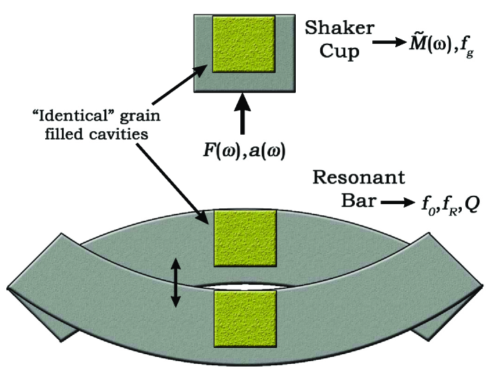
Figure 1: (Color online) Schematic of measurements: The effective mass, $\tilde{M}(\omega)$, is determined by simultaneously measuring the acceleration, $a(\omega)$, and force, $F(\omega)$, on an oscillating cup filled with grains. Using the measured $\tilde{M}(\omega)$ we show how to predict the acoustic properties of a resonance structure having the same grain-filled cavity. Here, $f_{g}$ represents a resonance frequency within the granular medium, $f_{0}$ represents the resonance frequency of the unloaded structure, and $f_{R}$ represents the resonance frequency of the loaded structure. In general, these resonance frequencies are complex-valued.

Next, in Section IV we discuss some rather general properties of the dynamic effective mass, considered as a causal response function. We analyze a model in which we treat the granular medium as a collection of rigid objects interacting via contact forces between them. We also analyze simple, continuum mechanical, models. Section V is devoted to an analysis of our data in the context of these continuum models which are useful for understanding features such as the main resonance, $f_{g}$, and the high frequency tail. Here, we analyze data on cavities filled with simple liquids, as well as data on our granular media. In order to get a sense of whether contact dampening or global dampening is the dominant mechanism in granular media we have performed a series of numerical simulations, which we report in Section VI. In Section VII we investigate the effect of differing humidities both on $\tilde{M}(\omega)$ and on the flex bar resonances. By means of these data it becomes clear that the dampening is local, due to the viscous adsorbed films of water in the contact region. We summarize our conclusions in Section VIII.

II Experimental Procedure

II.1 Effective Mass of Granular Media

A cylindrical cavity (of diameter 2.54 cm and height 3.07 cm) excavated in a rigid Al cup is filled with tungsten particles. Each of these particles consists of four or five equal-axis particles, of nominal size 100 $\mu$m, fused together. (See Figure 4, below.) The individual grains are far from being identical; using a micro-balance we measured the individual masses of 19 of these grains from which we deduce the average mass of an individual grain to be $m_{g}=44.2\pm 18.0\>\mu$g. The large density of tungsten maximizes the effects we are studying. The cup is subjected to a vertical sinusoidal vibration at angular frequency $\omega$; the resulting acceleration is measured with either one or two accelerometers attached to the cup, on the underside to one side of center (see below), and the force is measured with a force gauge mounted between the shaker and the cup. Taking into account the mass of the empty cup, $M_{c}$, we have

$$\tilde{M}(\omega)+M_{c}=\frac{F(\omega)}{a(\omega)},$$ (1)

where the effective mass of the granular medium, $\tilde{M}(\omega)=M_{1}(\omega)\>+\>iM_{2}(\omega)$, is complex-valued, reflecting the partially in-phase, partially out-of-phase motion of the individual grains, relative to the cup motion. As we shall see, $M_{1}$ may be conceptualized as an inertial effect, in the conventional sense, except that it depends upon an interplay between the masses of the individual grains and the stiffnesses of the grain-grain contacts; $M_{2}$ describes the attenuative aspects of the medium.

Of course, there is no such thing as a perfectly rigid cup. We have used a variety of different cups of slightly different geometries, with the intention that the apparent effect mass of the empty cup should be approximately frequency-independent. In Figure 2 we show the results for one such cup plotted over a fairly wide frequency range. We show both the empty cup data (dashed lines) and the filled cup data (solid lines). Depending upon the way in which the cup is filled with grains, either by slightly tapping on the cup (black curve) or by mechanically compacting the grains with press and plunger (green curve) we get quite different results, as discussed below. We note that the effective mass of the empty cup is essentially a frequency-independent constant, as expected. This result is a consequence of our use of two accelerometers on either side of the bottom of the cup, and taking the average. In either accelerometer there is a visible resonance structure around 6 (kHz), which seems to be a consequence of a “wobble” motion; the cup does not, literally, oscillate along a vertical axis. By averaging the two accelerometer signals, this wobble motion is effectively canceled. In this way we have improved on the technique reported in Ref. Hsu .

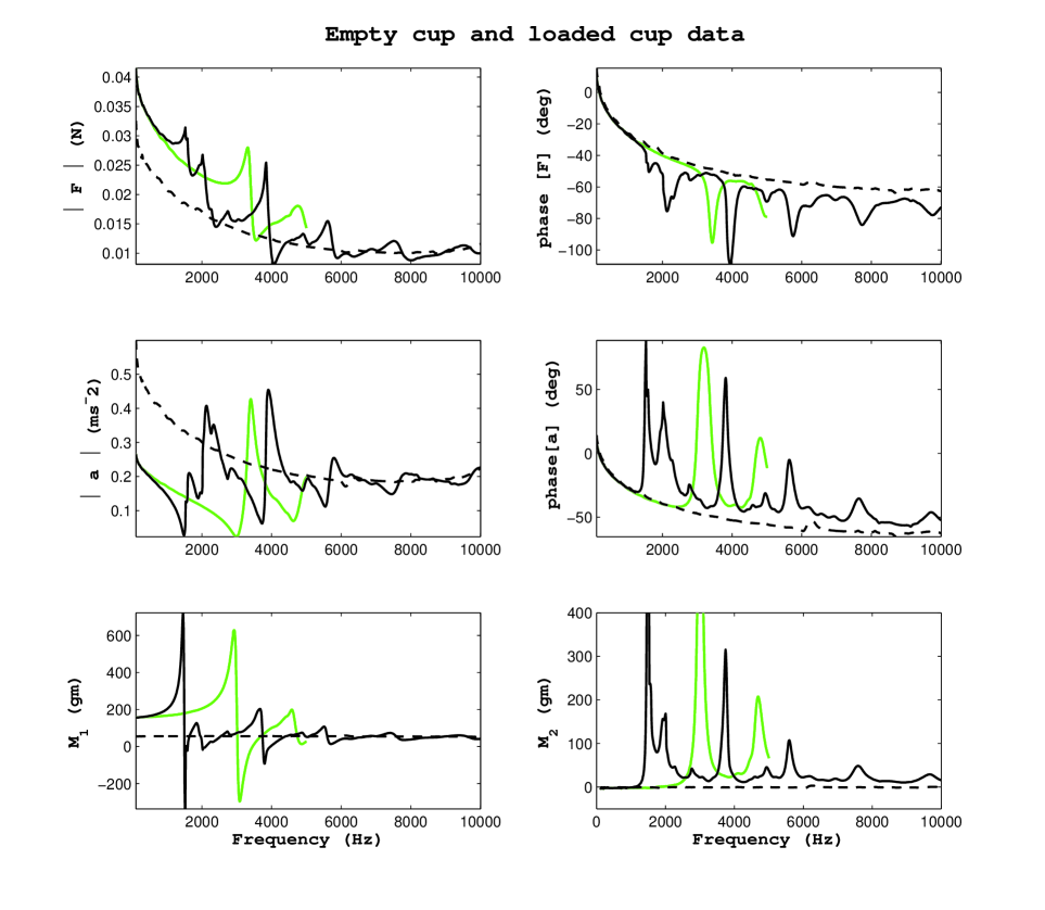
Figure 2: (Color online) Measurement results using one specific shaker cup over a wide frequency range. The top row represents the measured force, the middle row the acceleration, and the bottom row the effective mass. The left column represents the magnitude and the right column the phase relative to the driving voltage on the shaker, except that the bottom row shows the real, $M_{1}$, and the imaginary, $M_{2}$, parts of $\tilde{M}(\omega)$. The dashed curves represent the empty cup. The black curves are for a cup that was filled by simply tapping it whereas the green represents the mechanical compaction protocol, as described in the text. The measured effective mass of the empty cup, shown as a dashed curve, is essentially a frequency independent constant, which constant is subtracted from the total effective mass to yield that of the granular medium.

We note from Figure 2 that in the low frequency limit, $\tilde{M}(\omega)$ tends to the static mass of the grains. Also, there is a relatively sharp resonance peak whose position depends strongly on the manner in which the grains were prepared; there are also subsidiary resonances at higher frequencies. Although the data in Figure 2 are for the tungsten grains, we have shown previously that these general features of $\tilde{M}(\omega)$ are present in other granular media, such as spherical glass beads or spherical lead beads Hsu . In this article we focus on the tungsten granules, simply because the effect is maximal for such dense particles.

II.2 Resonant Bar

We consider the resonant frequencies of a rectangular bar of stainless steel whose dimensions are L X W X H = 20.32 cm X 3.81 cm X 3.18 cm. In the center of the top surface a cavity is excavated having virtually identical dimensions as that in the shaker cup (Figure 1). This cavity is filled with tungsten granules in the same manner and with the same mass as that held in the shaker.

We monitor the flexural modes of the system: The bar is suspended by wire supports attached at the approximate locations of the displacement nodes of the fundamental flex mode of the bar [Table 3.2 of reference Kinsler ]. The purpose here is to minimize any additional dampening in the experiment due to radiation of energy into the bar supports. On the top and on the bottom of the bar, near each of the ends, we epoxy piezoceramic disks of 6.35 mm diameter and 3.18 mm thickness. The two top disks are driven in phase with each other while the bottom two are driven out of phase with those on top. In this configuration the four disks act as a bending moment on the bar, thus inducing the desired flexural motion. We mount an accelerometer on the bottom directly under the center of the cavity. The bending moment is driven at a constant voltage as the frequency is swept in increments which are finely spaced when the Q is large (as for an empty cavity) and more coarsely spaced when the Q is low, as when the cavity is grain loaded. The output of the accelerometer, $a(\omega)$, shows a characteristic resonance peak as we sweep through the resonance.

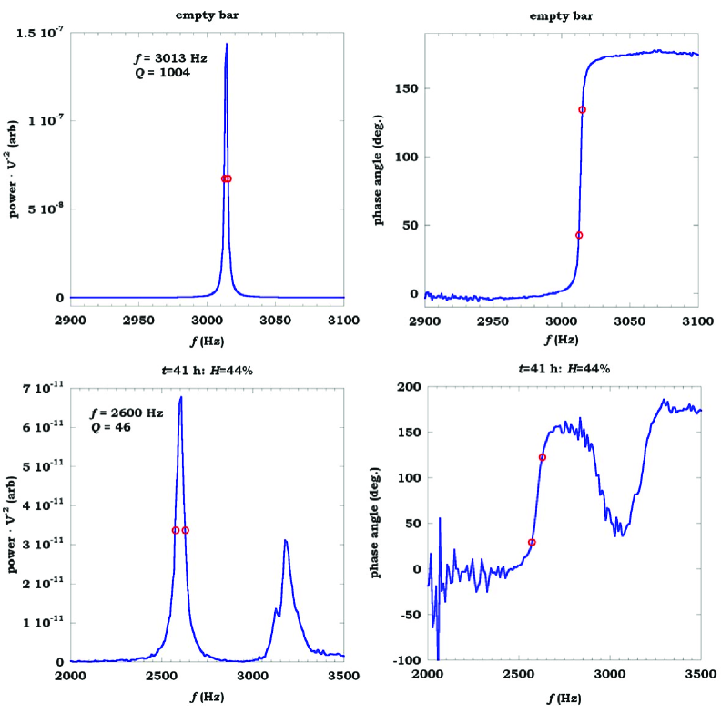
Figure 3: (Color online) Frequency scan of resonance in bar without (top) and with (bottom) tungsten granules. The dissipated power is plotted in the left column and the phase of the accelerometer, relative to the driving voltage on the benders, is plotted in the right. Note that, in this example, there are two distinct resonances in the granules loaded bar. The red circles mark the frequencies at which the power is equal to half its peak value. Note that there is a $90^{o}$ degree phase shift between the two half-max points, as expected.

We take the power dissipated in the vibrating bar to be $\mathcal{P}(\omega)\propto\;\mid a(\omega)\mid^{2}/\omega^{2}$. This quantity is plotted, in arbitrary units, in Figure 3. The real part of the resonance frequency, $f_{R}$, and the quality factor, Q, may be taken from the peak and the full-width at half maximum of this curve. See pages 23 ff. of Kinsler and Frey Kinsler .

This technique of finding $f_{R}$ and $Q$ works well when there is an isolated peak and the background power absorption is small. However, in many cases during our experiments there are two nearby peaks with significant overlap between them and/or there is a significantly large background absorption. For such situations there are established procedures for extracting $f_{R}$ and Q. They assume specific functional forms for the response function in which the parameters therein are adjusted to achieve a best fit to the response data mehl . We have taken a different approach which assumes only that the data represents a sampling on the real axis of an analytic function of complex frequency.

We record the complex-valued data for the acceleration of the bar, $a(\omega_{i})$, as we do for the cup, where $\{\omega_{i}\}$ is the set of discrete measurement frequencies. We analytically continue the auxiliary function $g\stackrel{{\scriptstyle def}}{{=}}1/a$ using a rational function technique (Bulirsch-Stoer algorithm) numrec (See also Appendix B). It is relatively simple to search for a zero of this analytically continued function [$g(\omega_{R})=0$] using Muller’s method numrec . We have

$$\omega_{R}=2\pi f_{R}[1-i/(2Q)]=2\pi f_{R}-i\alpha\>\>\>,$$ (2)

where $\alpha$ is the decay rate of the mode. We find that this technique is highly reliable. As far as we are aware, it has not previously been reported in the literature.

We see from Figure 3 that there is a very significant effect due to the addition of the loose grains. When the cavity is empty, and the frequency scanned with 0.5 (Hz) increments, we find that, in the range $100{\rm(Hz)}<f<5{\rm(kHz)}$, there is only a single resonance: $f_{0}({\rm empty\>bar})=3014\>{\rm(Hz)}\pm 0.1\%$ and ${\rm Q}_{0}(\rm{exp})=1004\pm 15\%$. When the cavity is filled with the tungsten particles, and the bar is scanned in 10 (Hz) frequency increments, there is a significant frequency shift for the main resonance, $f_{R}({\rm loaded})=2600\>{\rm(Hz)}$, and increase in attenuation: ${\rm Q}_{R}(\rm{loaded})=46$. It is this latter feature that makes granular dampening an attractive possibility for reducing unwanted structure-borne sound. Moreover, there is a new, additional mode that is not present in the unloaded bar. The major thrust of this article is that these resonant bar characteristics can be computed directly, based on the measured effective mass, $\tilde{M}(\omega)$; a detailed comparison between theoretical predictions and experimental results, as a function of humidity, is presented later in Section VII.2 using a theory developed in Appendix A.

II.3 Sample Handling

A major concern for us is that we need to be able to prepare the loose grains in the two cavities in a reproducible manner. This will allow us to make meaningful predictions about the resonant properties of the bar, using the measured effective mass in the shaker cup. Granular media are notoriously hard to prepare reproducibly because they often configure themselves into meta-stable states. For spherical grains it is relatively easy to get the grains into a state approximating random close packing, whose properties are quite reproducible sphere_pack . Our granular systems, however, do not lend themselves easily to this. This is because each granule consists of several sand-grain like particles fused together. A photomicrograph of a few of these granules is shown in Figure 4. Although the main features of the effective mass are certainly reproducible, the details of the structure in $\tilde{M}(\omega)$ can vary significantly enough from one filling to the next that, unless precautions are taken, it prevents an accurate theory-experiment comparison in the bar.

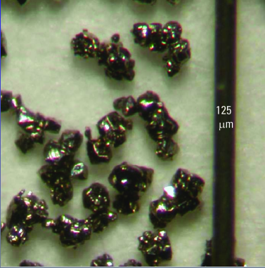
Figure 4: (Color online) Photomicrograph of some tungsten granules used in the experiment. There is a 125 $\mu$m wire at the right, for comparison.

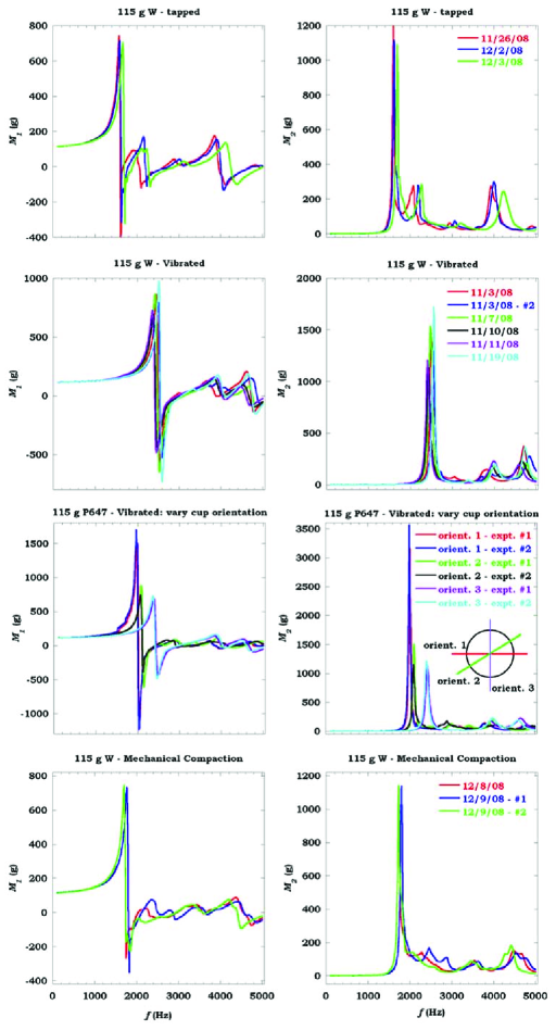
Figure 5: (Color online) Effective mass, $\tilde{M}(\omega)$, measured on subsequent packings of the shaker cup using four different loading protocols. First Row: simple filling and subjective tapping. Second Row: Sinusoidal vibration, aligned cup. Third Row: Sinusoidal vibration, different cup orientations. Fourth Row: Mechanical compaction with commercial press.

In Figure 5 we show the reproducibility of the effective mass for consecutive runs using each of the different protocols. In the first row we show the results of filling while occasionally tapping to settle the grains. Next, we show the result of vibrating the particulate medium at a frequency of 1 (kHz) over a range of acceleration amplitudes, $0<a<30\;(m\cdot s^{-2})$ with a 93 g stainless steel plug resting on the free surface. The plug ensures that the grains at the surface experience a static pressure similar to that experienced at the bottom of the particle pack. The protocol consists of systematically increasing the acceleration amplitude in steps of 5 $(m\cdot s^{-2})$, holding for 2 min at each amplitude before increasing to the next level. After reaching the maximum acceleration amplitude [$30\;(m\cdot s^{-2})$] the procedure is reversed. Therefore, the sample is exposed to 6 different acceleration amplitudes, and the protocol consists of 11 total steps. The procedure is similar to that employed by Nagel et al. sphere_pack .

The results indicate that vibrating the sample with a mass on the free surface yields a fairly consistent $\tilde{M}(\omega)$. All of the samples exhibit the same features, and these features are observed at relatively consistent frequencies. The main resonance in the grains is observed to occur over a slightly broader frequency band (2.4 - 2.6 (kHz)) than that observed when the sample is tapped. On the other hand, compared to that observed after the sample is tapped there appears to be slightly better reproducibility in the shape and position of the secondary features. It is interesting to note that the higher degree of compaction achieved with the vibration protocol shifts the main resonance to higher frequency, as compared to that observed with the tapping protocol. In Section V.2 we will see that this shift can be interpreted as an increase in effective sound speed in the granular medium.

Unfortunately, while reproducible, the effective mass so obtained with this protocol varies with the orientation of the cup relative to the shaker on which it is mounted. This effect is demonstrated in the third row of Figure 5. The effective mass is reproducible for a single orientation, but it varies with orientation. Evidently the wobble effect we discussed earlier is big enough to effect the packing of the grains, when we vibrate at these high amplitudes. Therefore, the vibration protocol is not optimal for handling the samples prior to a transferability experiment because we cannot insure that we can duplicate the motion of the bar and the cup as we vibrate it at high amplitudes during the preparation phase.

The most successful method for developing a reproducible loading was to mechanically compact the grains after they had been loaded in their respective cavities. This protocol consists of using a mechanical testing instrument to impose a sinusoidal stress on the free surface. To promote a uniform imposition of the stress over the free surface of the grains, we use a stainless steel plunger with a rubber pad glued to the bottom surface. First, a static stress of 59.2 (kPa) is imposed on the granular medium. Then, a sinusoidal stress is imposed on the system consisting of 200 cycles at a frequency of 0.25 (Hz). The stress amplitude is systematically varied between 39.5 (kPa) and 118.5 (kPa), in steps of 39.5 (kPa). To prevent unloading the system, the static stress is increased by 39.5 (kPa) for each equivalent change in stress amplitude. After the maximum stress amplitude is achieved, the procedure is repeated in reverse. So the first two steps consist of increasing, and the second two steps consist of decreasing the stress amplitude. We have limited the maximum stress on the grains to the low value of 118.5 (kPa) [= 1.185 (bar)] specifically in order to ensure that we are not physically damaging any of the grains. Overall the system is exposed to 1000 stress cycles (5 sets of 200) at systematically varied stress amplitudes. In order to test the reproducibility of this protocol we have repeated the measurement by dumping out the grains, repacking the same amount by weight of fresh grains using the compaction technique, measuring $\tilde{M}(\omega)$, dumping out the grains, repacking, etc. For the purposes of comparing theory vs. experiment in the bar data [Section VII.2], we used the mechanical compaction protocol.

III Dampening of Structure-Borne Sound and the Effective Mass of Granular Media

Subject to the validity of a few simple assumptions, it is possible to use the measured effective mass, $\tilde{M}(\omega)$, to compute its dampening effect on an elastic structure having an “identical” grain-filled cavity. Let us suppose that there is an acoustic structure which has a resonant frequency $\omega_{0}$ when the cavity is empty. The resonant frequency becomes complex-valued in the presence of the granular dampening mechanism: $\omega=\omega_{0}+\Delta\omega$. Here, ${\rm Imag}(\omega)$ describes the ring-down rate of the mode in the time domain or, equivalently, the quality factor of the resonance in the frequency domain: Q $=-{\rm Re}(\omega)/[2\>{\rm Im}(\omega)]>0$. We make the approximation that the grains contribute an additional mass-loading which is localized at position ${\bf x_{1}}$. Thus, the density may be written as

$$\rho({\bf x})=\rho_{0}({\bf x})+\tilde{M}(\omega)\delta({\bf x-x_{1}})$$ (3)

where $\rho_{0}({\bf x})$ is the point-by-point density of the structure when the cavity is empty. This assumption is essentially a statement that we are considering only those normal modes of the structure whose wavelengths are much larger than the dimensions of the cavity. We make the further assumption that the grain-filled cavity contributes negligibly to any change in the effective elastic moduli of the host structure. i.e. The effective moduli of the grains, as seen by the walls of the cavity, are much smaller than those of the host material. In Section V.2 we show that this is an excellent approximation for the effective masses and structures we are considering here.

The equations of elasto-dynamics may now be recomputed using this modified, and now frequency dependent and complex-valued, density. We demonstrate how to do this sort of computation for the specific case of the fundamental flex mode in a rectangular bar in Appendix A.

It is most useful, however, to consider the results of the much simpler perturbation theory, which is valid to first order in $\tilde{M}(\omega)$, considered as a small perturbation. The displacement field obeys the usual equations of motion:

$$-\rho\lambda u_{i}=[C_{ijkl}u_{k,l}]_{,j}\>\>\>.$$ (4)

Here, $\rho$ and $C_{ijkl}$ are the position dependent density and elastic constants of the material, $u_{i}({\bf x})$ is the $i$-th component of the displacement field, a comma denotes differentiation w.r.t that coordinate, and summation over repeated indices is understood; $\lambda\equiv\omega^{2}$ is the eigenvalue for the problem. Written in this manner, Equation (4) applies to any position-dependent material constants, $\rho({\bf x})$ and $C_{ijkl}({\bf x})$, including those with step discontinuities. We consider resonances such that either the displacement field vanishes on the boundary surface of the structure, ${\bf u}\mid_{S}\equiv 0$, or the stress tensor vanishes on that surface, $C_{ijkl}u_{k,l}\mid_{S}\equiv 0$. Moreover, we assume that the elastic constants, $C_{ijkl}$, and the unperturbed density, $\rho_{0}$, are real-valued, thus guaranteeing that $\omega_{0}$, the resonance frequency when there are no grains in the cavity, is also real-valued.

Now, if the density is perturbed to take on a new value, $\rho=\rho_{0}+\Delta\rho$ then there is a corresponding change in both the eigenvalue $\lambda=\lambda_{0}+\Delta\lambda$, and in the eigenvector, ${\bf u}={\bf u}^{0}+\Delta{\bf u}$. Substituting into Eq. (4) and collecting all the first order changes one has

$$-\Delta\lambda\rho_{0}u^{0}_{i}-\lambda_{0}\rho_{0}\Delta u_{i}-\lambda_{0}\Delta\rho u^{0}_{i}=[C_{ijkl}\Delta u_{k,l}]_{,j}\>\>\>.$$ (5)

Multiply Eq. (5) by $[u^{0}_{i}]^{*}$ (sum on $i$) and integrate over all space. The term $\int[u^{0}_{i}]^{*}[C_{ijkl}\Delta u_{k,l}]_{,j}\>dV$ can be integrated by parts; the surface term vanishes because of the assumed boundary condition (above). The remaining volume integral cancels the term $-\lambda_{0}\int\rho_{0}[u^{0}_{i}]^{*}\Delta u_{i}\>dV$ (because ${\bf u}_{0}$ satisfies the zero-order equation). Thus,

$$\Delta\lambda=-\frac{\lambda_{0}\int\Delta\rho{(\bf x})\mid{\bf u^{0}(x)}\mid^{2}\>dV}{\int\rho_{0}({\bf x})\mid{\bf u^{0}(x)}\mid^{2}\>dV}\>\>\>.$$ (6)

Applied to the case of interest, Eq. (3) for which $\Delta\rho({\bf x})=\tilde{M}(\omega)\delta({\bf x-x_{1}})$, this now reads:

$$\Delta\omega=-\left[\frac{\omega_{0}I_{1}}{2M_{0}}\right]\tilde{M}(\omega_{0})\>\>\>.$$ (7)

where

$$I_{1}=\frac{M_{0}\mid{\bf u^{0}(x_{1})}\mid^{2}}{\int\rho_{0}({\bf x})\mid{\bf u^{0}(x)}\mid^{2}\>dV}\>\>\>,$$ (8)

in which ${\bf u^{0}(x)}$ is the displacement field, and $\rho_{0}({\bf x})$ is the density, when the cavity is empty of grains. $M_{0}=\int\rho_{0}({\bf x})\>dV$ is the total mass of the structure when there are no grains in the cavity. Written in this manner, $I_{1}$ is dimensionless. In order for this sort of theory to be valid, the granular media in the two cavities must be substantially the same. In Section VII.2 we make such a theory-experiment comparison, but we have had to go beyond the simple perturbation theory result for two reasons: (1) The effective mass, $\tilde{M}(\omega)$, is not always small. It can, in fact, take on values larger than that of the steel bar. Perturbation theory cannot give an accurate description in these cases. (2) Some of the modes seen in the bar + grains system are basically modes within the grains [i.e. poles of $\tilde{M}(\omega)$] modified by the effect of the bar. Perturbation theory is silent as to the properties of these modes. Nonetheless, for the modes which are primarily bar-like, Equation (7) gives a useful intuitive way to think about the effects of the granular medium on the resonance frequency and Q. Specifically, $M_{1}(\omega_{0})$ determines the shift in the resonance frequency and $M_{2}(\omega_{0})$ determines the lowered Q, as is clear from Equation (7).

We note in passing that the effective mass is, in reality, a tensor, viz $\tilde{M}_{ij}(\omega)$, reflecting the fact that gravity plays a major role in establishing stiffness and dampening at the contacts. Equation (4) has an obvious generalization to the case of a tensorial density and Equation (7) becomes

$$\Delta\omega=-\frac{\omega_{0}u_{i}^{0*}(x_{1})\tilde{M}_{ij}(\omega_{0})u^{0}_{j}(x_{1})}{2\int\rho_{0}({\bf x})\mid{\bf u^{0}(x)}\mid^{2}\>dV}\>\>\>.$$ (9)

In this article we are considering only situations in which the cavity motion is strictly along the z-axis, parallel to the force of gravity. Thus the only relevant component of the effective mass being considered here is $\tilde{M}_{zz}(\omega)$ which we shall henceforth denote without the subscripts, but with this understanding that there are other nonzero components of the tensor.

IV Properties of $\tilde{M}(\omega)$

In this Section we first discuss some general properties of $\tilde{M}(\omega)$ considered as a causal response function. Next, we investigate some properties of the system in which we idealize the grains as being rigid particles which interact with their neighbors via contact forces, of which there may be different kinds. A specific motivation here is to analyze the high frequency behavior seen in our own measurements of $\tilde{M}(\omega)$ within this discrete particles context. Finally, some of the features we observe in $\tilde{M}(\omega)$ are suggestive of a collective motion in which the displacement varies slowly from grain to grain. This suggests the possible approximate validity of continuum models, two of which we present here.

IV.1 General

The effective mass, $\tilde{M}(\omega)$, is a causal response function in that one may, in principle, apply an arbitrary time-based protocol to the acceleration of the cup and measure the force induced by this protocol. As such it has several general properties, which we summarize here. These properties follow on general principles as described in e.g. Landau and Lifshitz landau . $\tilde{M}(\omega)$ is the fourier transform of a real-valued memory function:

$$\tilde{M}(\omega)=\int_{0}^{\infty}\chi(t)e^{i\omega\tau}\>d\tau\>\>\>.$$ (10)

Causality considerations specifically restrict the range of integration to positive values of $\tau$ only. That is, in the time domain, the force and the acceleration are related to each other via the memory function, $\chi(t)$:

$$F(t)=\int_{0}^{\infty}\chi(\tau)a(t-\tau)\;d\tau\>\>\>.$$ (11)

Inasmuch as only the past history of the acceleration matters in Equation (11) its fourier transform leads to Equation (10). If the frequency, $\omega$, is extended to take on complex values, we see that $\tilde{M}(\omega)$ is regular everywhere in the upper-half complex plane. We also see from Eq. (10) that

$$\tilde{M}(-\omega*)=\tilde{M}^{*}(\omega)\>\>\>,$$ (12)

where an asterisk signifies complex conjugation. These considerations lead immediately to the usual Kramers-Kronig relations between the real and the imaginary parts:

$$M_{1}(\omega)=\frac{2}{\pi}P\left[\int_{0}^{\infty}\frac{xM_{2}(x)}{x^{2}-\omega^{2}}dx\right]$$ (13)

$$M_{2}(\omega)=-\frac{2\omega}{\pi}P\left[\int_{0}^{\infty}\frac{M_{1}(x)}{x^{2}-\omega^{2}}dx\right]\>\>\>,$$ (14)

where $\omega$ and $x$ take on real values only and $P[\>]$ denotes principal part of the argument. (We are assuming there are no singularities on the real axis and that $\lim_{\omega\rightarrow\infty}\tilde{M}(\omega)=0$. See Section IV B, below.)

One may just as well consider a time-based protocol for an applied force and measure the induced acceleration of the cup. Therefore $1/\tilde{M}(\omega)$ is also a causal response function and all the results quoted above apply to it as well, except for the Kramers-Kronig relations. Thus, $\tilde{M}(\omega)$ has no zeroes, poles, branch points, or singularities of any kind anywhere in the upper half plane. Inasmuch as only the constant functions are analytic and bounded everywhere in the complex plane, $\tilde{M}(\omega)$ must have singularities of some sort in the lower-half plane.

The power dissipated in the system, averaged over one cycle of oscillation, is

$$\begin{array}[]{rcl}\mathcal{P}&=&\langle Re[F]Re[v]\rangle\\ &&\\ &=&(1/2)Re[F\;v^{*}]\\ &&\\ &=&(1/2)\;\omega M_{2}(\omega)\mid v\mid^{2}\>\>\>,\end{array}$$ (15)

where $v=ia/\omega$ is the velocity of the cup. Since $\mathcal{P}$ is always non-negative, one has $\omega M_{2}(\omega)\geq 0$, for real values of the frequency. We see that this property is borne out by the data in Figures 2 and 5.

IV.2 Systems of Discrete Particles

Let us consider a model in which each grain is considered to be rigid except for the region near the contacts with its neighboring particles. Let ${\bf X}_{i}$ be the equilibrium position of the center of mass of the i-th particle, whose mass is $m_{i}$, and ${\bf u}_{i}$ be its displacement from equilibrium. Similarly, ${\mbox{\boldmath{$\theta$}}}_{i}$ is the librational angle of rotation. If two neighboring particles translate or rotate such that their points of contact would move relative to each other there will be a restoring force due to the contact forces. The linearized equation of motion for the i-th particle is

$$\begin{array}[]{c}-m_{i}\omega^{2}{\bf u}_{i}=-{\bf K}_{iw}\cdot[{\bf u}_{i}+{\mbox{\boldmath{$\theta$}}}_{i}\times{\bf d}_{iw}-{\bf W}]\\ \\ +\sum_{j}{\bf K}_{ij}\cdot[{\bf u}_{j}+{\mbox{\boldmath{$\theta$}}}_{j}\times{\bf d}_{ji}-{\bf u}_{i}-{\mbox{\boldmath{$\theta$}}}_{i}\times{\bf d}_{ij}]\\ \end{array}\;\;\;,$$ (16)

where ${\bf d}_{ij}$ is the vector from ${\bf X}_{i}$ to the point of contact with the j-th grain. It is understood that the tensor ${\bf K}_{ij}(\equiv{\bf K}_{ji})$ is nonzero only for grains actually in contact with each other. (We assume there is at most one contact per pair.) Similarly, ${\bf d}_{iw}$ and ${\bf K}_{iw}$ refer to grains that are in contact with the surfaces of the cavity, whose rigid displacement is ${\bf W}$.

The equation of motion for the angular variables is

$$\begin{array}[]{c}-\omega^{2}{\bf I}_{i}\cdot{\mbox{\boldmath{$\theta$}}}_{i}=-{\bf d}_{iw}\times{\bf K}_{iw}\cdot[{\bf u}_{i}+{\mbox{\boldmath{$\theta$}}}_{i}\times{\bf d}_{iw}-{\bf W}]\\ \\ +\sum_{j}{\bf d}_{ij}\times{\bf K}_{ij}\cdot[{\bf u}_{j}+{\mbox{\boldmath{$\theta$}}}_{j}\times{\bf d}_{ji}-{\bf u}_{i}-{\mbox{\boldmath{$\theta$}}}_{i}\times{\bf d}_{ij}]\end{array}\;\;\;,$$ (17)

where ${\bf I}_{i}$ is the moment of inertia tensor for the i-th particle.

In the special case that the particles are identical spheres we have ${\bf d}_{ij}=(1/2)[{\bf X}_{j}-{\bf X}_{i}]$ and the spring constant tensor may be written in terms of normal (N) and transverse (T) stiffnesses as

$${\bf K}_{ij}=k_{ij}^{N}\hat{{\bf d}}_{ij}\hat{{\bf d}}_{ij}+k_{ij}^{T}[{\bf I}-\hat{{\bf d}}_{ij}\hat{{\bf d}}_{ij}]\;\;\;,$$ (18)

where $\hat{{\bf d}}_{ij}$ is the unit vector and we use dyadic notation. Similarly for the contacts with the walls. An example here would be Hertz-Mindlin contact forces in which the stiffnesses increase with increasing static compression but we also consider forces of adhesion, capillarity, etc.

It is understood that, generally, each of the elements of the tensors ${\bf K}_{ij}$ or ${\bf K}_{iw}$ are complex-valued and frequency dependent reflecting the microscopic origin of the dissipation. For example, one may take

$${\bf K}_{ij}(\omega)={\bf K}_{ij}^{0}-i\omega{\bf B}_{ij}$$ (19)

in which the second term describes an inter-particle force proportional to the difference in velocity of the two grains. The tensor ${\bf B_{ij}}$ is analogous to a dampening parameter. In general Eq. (19) represents simply the first two terms in the Taylor’s series expansion of ${\bf K}(\omega)$. These “springs” may have rheological properties of their own. For example, if there is an internal degree of freedom with relaxation time $\tau$ it is easy to show that

$${\bf K}_{ij}(\omega)={\bf K}_{ij}^{\infty}+\frac{{\bf K}_{ij}^{0}-{\bf K}_{ij}^{\infty}}{1-i\omega\tau}\;\;\;.$$ (20)

The derivation of Eq. (20) parallels that of Eq. (78.6) in Landau and Lifshitz llfm . A Taylor’s series expansion of Eq. (20) for small $\omega$ has the form of Eq. (19) for the first two terms.

Notwithstanding the foregoing remarks there are some general conclusions one can draw from Eqs. (16) and (17). First, the total force which the cavity exerts on the grains is

$$\begin{array}[]{rcl}{\bf F}&=&-\sum_{i}{\bf K}_{iw}\cdot[{\bf u}_{i}+{\mbox{\boldmath{$\theta$}}}_{i}\times{\bf d}_{iw}-{\bf W}]\\ &&\\ &=&-\omega^{2}\sum_{i}m_{i}{\bf u}_{i}\;\;\;,\end{array}$$ (21)

where the second equality follows because the interparticle forces cancel, by Newton’s third law, as is clear from Eq. (16). Secondly, one can formally write the effective mass in terms of the normal-mode frequencies of the system:

$$\tilde{{\bf M}}(\omega)=\sum_{n}\frac{{\bf A}_{n}}{\omega-\omega_{n}}$$ (22)

where $\omega_{n}$ are the complex-valued frequencies for which Eqs. (16) and (17) have nontrivial solutions when ${\bf W}$ is set equal to zero. Each matrix ${\bf A}_{n}$ represents the strength of each resonance. Also, from Eqs. (16) and (17) it is clear that when the frequency tends to zero one has $\lim_{\omega\rightarrow 0}{\bf u}_{i}={\bf W}$ and $\lim_{\omega\rightarrow 0}{\mbox{\boldmath{$\theta$}}}_{i}=0$. Therefore, in this limit one has, from the second of Eq. (21), ${\bf F}=-\omega^{2}M_{0}{\bf W}$ where $M_{0}=\sum_{i}m_{i}$ is the total static mass of the grains. Therefore, from the definition of the effective mass, one has:

$$\lim_{\omega\rightarrow 0}\tilde{{\bf M}}(\omega)=M_{0}{\bf I}\;\;\;,$$ (23)

which seems obvious.

The high frequency limit of the effective mass also has a simple form. From Eqs. (16) and (17) one has $\lim_{\omega\rightarrow\infty}{\bf u}_{i}=0$ and $\lim_{\omega\rightarrow\infty}{\mbox{\boldmath{$\theta$}}}_{i}=0$, because of the dominance of inertial effects. i.e. The particles do not move at all, in this limit. Therefore, in this limit the first of Eq. (21) implies ${\bf F}=\sum_{i}\lim_{\omega\rightarrow\infty}{\bf K}_{iw}(\omega)\cdot{\bf W}$ which, in turn, implies

$$\lim_{\omega\rightarrow\infty}\tilde{\bf M}(\omega)=-\frac{\lim_{\omega\rightarrow\infty}\sum_{i}{\bf K}_{iw}(\omega)}{\omega^{2}}\>\>\>.$$ (24)

The high frequency behavior of $\tilde{\bf M}(\omega)$ is controlled by the behavior of those “springs” connecting the particles directly to the cavity motion. If, for example, these are strictly dampened springs, such as implied by Eq. (19), then

$$\lim_{\omega\rightarrow\infty}\tilde{\bf M}(\omega)=i\frac{\sum_{i}{\bf B}_{iw}}{\omega}\>\>\>,$$ (25)

which is predominantly imaginary valued in this limit. On the other hand, if the individual springs have their own rheological behavior, such as that implied by Eq. (20), then

$$\lim_{\omega\rightarrow\infty}\tilde{\bf M}(\omega)=-\frac{\sum_{i}{\bf K}_{iw}^{\infty}}{\omega^{2}}\>\>\>.$$ (26)

Should this latter case hold then comparison with Eq. (13) immediately gives an f-sum rule on the absorptive part of the effective mass:

$$\int_{0}^{\infty}\omega\>{\rm Imag}[{\tilde{\bf M}}(\omega)]\;d\omega=\frac{\pi}{2}\sum_{i}{\bf K}_{iw}^{\infty}\>\>\>.$$ (27)

So if those grains that are in contact with the walls of the cavity have spring constants which are real-valued in the high frequency limit then the integrated absorptive part of the effective mass is determined solely by those high frequency spring constants, independent of the details of the grain-grain contact forces.

The potential usefulness of the results of this subsection is that the high frequency limit of the measured $\tilde{M}(\omega)$ may be compared against Eqs. (24) and its variants. In our own experiments we are not able to probe frequencies high enough to observe this behavior, as discussed in Section V.2, below.

IV.3 Continuum Models

On a semi-quantitative level, we may understand the general features of our experimental results, such as those in Figures 2 and 5, in terms of two over-simplified continuum models whose main purpose will be to allow us to deduce approximate parameter values from our data.

Model I: The granular medium is considered to be a lossy fluid, with negligible viscous effects at the walls; that is, the viscous skin depth landau $\delta=\sqrt{2\eta/(\rho\omega)}$ is small compared to the radius of the cup, $a$. Here, $\eta$ is the viscosity of the fluid; $\rho$ is the density. The effective mass is simply

$$\tilde{M}(\omega)=M_{0}\tan(qL)/(qL)\>\>\>,$$ (28)

where $L$ is the height of the fluid column, $q=\omega\sqrt{\rho/K}$ is the wave vector in the fluid in terms of a (lossy) bulk modulus, $K=K_{0}[1-i\omega\tau]$. $M_{0}=\pi a^{2}L\rho$ is the static mass in the cup. This model presupposes that 100% of $\tilde{M}(\omega)$ is supported by the bottom surface of the cup. For “small enough” values of the damping parameter, $\tau$, resonance peaks, as seen in Figure 6a, occur when $qL$ equals odd multiples of $\pi/2$ i.e. L equals odd multiples of 1/4 wavelength: $L=\lambda/4,3\lambda/4,5\lambda/4.\cdots$ These sharp resonances are examples of $f_{g}$, the resonances within the granular medium/liquid. The values of $K_{0}$ and $\tau$ are chosen to mimic the observed frequency position and resonance width, respectively, in the experiments. There is a second resonance in Figure 6a around 4500 (Hz), but the width of that resonance is nines times as large as the first one, so it is scarcely visible in the plot.

We emphasize that this last feature, the resonance frequencies being in the ratio 1:3:5:7 …, is an artifact of three assumptions in Model I: (a) There is no shear rigidity or shear viscosity in the material. (b) The sound speed is constant throughout the sample. (c) The attenuation parameter, $\tau$, is small. We shall see that all of these assumptions are violated, strictly speaking, under the conditions of our experiments on real granular media.

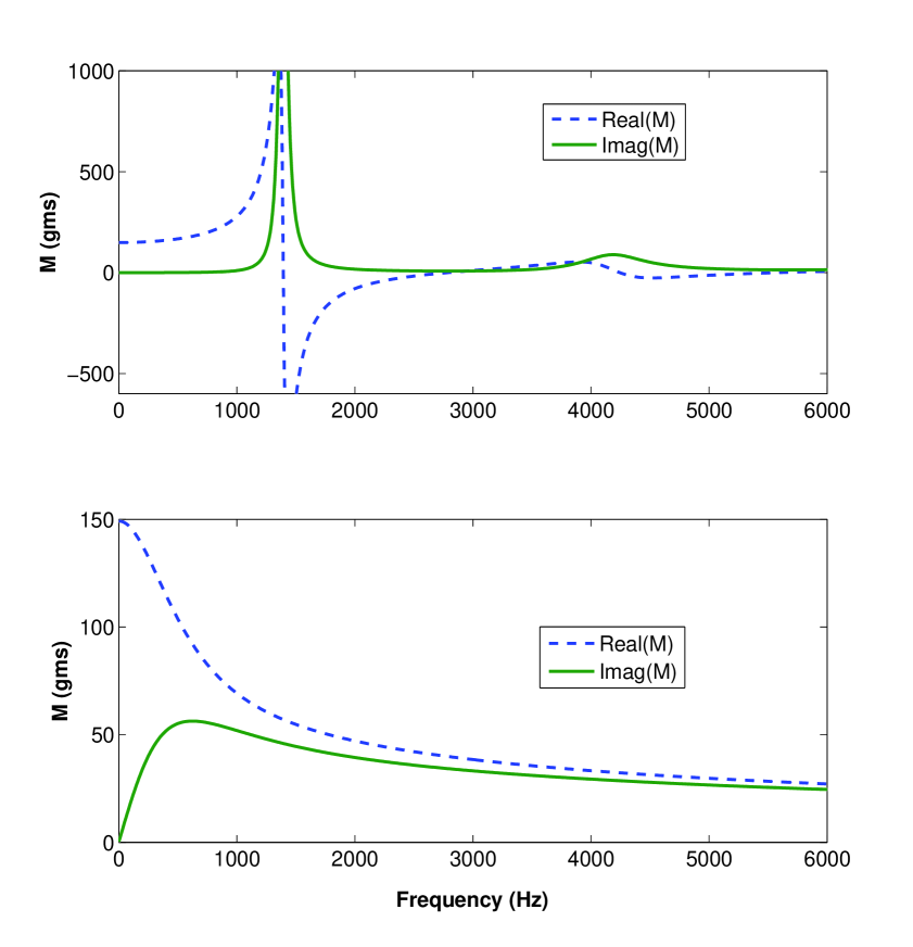
Figure 6: (Color online) (Top) Model I, a fluid with a lossy bulk modulus. (Bottom) Model II, a highly compressible, highly viscous fluid.

Model II: The granular medium is considered to be a very viscous fluid, which is infinitely compressible. This situation may be approximately correct if the filling depth of the cavity is much greater than the diameter so that most of $\tilde{M}(\omega)$ is borne by the walls of the cup, little by the bottom surface. By solving the Navier-Stokes equation for oscillatory motion in a cylindrical geometry landau we find

$$\tilde{M}(\omega)=2M_{0}J_{1}(\kappa a)/[\kappa aJ_{0}(\kappa a)].$$ (29)

Here $\kappa=\sqrt{i\rho\omega/\eta}$, and $J_{k}(z)$ is a Bessel function of order $k$. This model gives a broad peak with a slow decay at higher frequencies as seen in Figure 6b, much like that seen qualitatively in the granular data above the fundamental resonance. We note, for future use, that the high frequency limit of Eq. (29) is

$$\tilde{M}(\omega)\rightarrow 2\pi aL\sqrt{i\eta\rho/\omega}\>\>\>.$$ (30)

This limit holds when the viscous skin depth llfm , $\delta=\sqrt{2\eta/\rho\omega}$ , is much smaller than the radius of the cup. We suppose, then, that the result $\tilde{M}(\omega)\propto\sqrt{i/\omega}$ holds generally, for other geometries, but with different prefactors.

Is the high-frequency limit for this continuum model consistent with what one might expect for a discrete system of particles, with dampening due to their relative motion, namely Eq. (25)? Though one may expect viscous-like dampening analogous to that described by Eq. (30), at high enough frequencies the viscous skin depth becomes small compared to the inter-particle separation and there is a crossover from $\tilde{M}\propto(1+i)\omega^{-1/2}$ to $\tilde{M}\propto i\omega^{-1}$. This can be demonstrated explicitly if one considers a one-dimensional string of point masses, separated a distance $b$ from each other, each of which experiences a drag force proportional to the difference between its velocity and its neighbor’s, viz: $F=\gamma[v_{j}-v_{i}]$. This leads to the equation of motion for the ensemble:

$$-m\omega^{2}u_{j}=-i\omega\gamma(u_{j+1}-2u_{j}+u_{j-1})\>\>\>j=-N,...N$$ (31)

subject to the boundary condition

$$u_{\pm(N+1)}=W\>\>\>.$$ (32)

Equation (31) is a simple example of Equation (19) in which $B_{ij}=\gamma$ if $i$ and $j$ are nearest neighbors and $K_{ij}\equiv 0$. It is simple enough to solve for the effective mass implied by this toy model. Let

$$y_{\pm}=\frac{2\gamma-im\omega\pm i\sqrt{m^{2}\omega^{2}+4im\omega\gamma}}{2\gamma}\>\>\>.$$ (33)

The dynamic effective mass of one such row is

$$\tilde{M}_{1D}(\omega)=\frac{2i\gamma}{\omega}\left[\frac{y_{+}^{N+1}+y_{-}^{N+1}-y_{+}^{N}-y_{-}^{N}}{y_{+}^{N+1}+y_{-}^{N+1}}\right]\>\>\>.$$ (34)

If we imagine that there is a sequence of these chains, in parallel with each other, all connected to the walls then Eq. (31) is a discretized version of the linearized Navier-Stokes equation for which the viscosity is $\eta\propto\gamma b$. The effective mass per unit area of the side wall implied by the continuum Navier Stokes equation in this geometry is

$$\tilde{M}_{NS}(\omega)/A=\frac{2\rho}{\kappa}\tan(\kappa T/2)\>\>\>,$$ (35)

where $T$ is the separation between the walls. Equation (35) has a high-frequency limit analogous to Equation (30):

$$\tilde{M}_{NS}(\omega)/A\rightarrow 2\sqrt{i\eta\rho/\omega}\>\>\>.$$ (36)

Taking into account the appropriate normalization of the relevant constants one may directly compare Eq. (34) against Eq. (35). This is done in Figure 7 where we plot the imaginary part of the effective mass implied by each of the models. They agree with each other over much of the frequency range. The peak around 300 (Hz) occurs when the viscous skin depth is approximately equal to the wall separation, $T$. Above that frequency each model has a frequency dependence $\tilde{M}_{2}\propto\omega^{-1/2}$, as expected from Eq. (36). When, however, the macroscopic viscous skin depth, $\delta=\sqrt{2\eta/\rho\omega}$, is approximately equal to the inter-particle separation, $b$, the discrete model, Eq. (34), crosses over to a behavior implied by Eq. (25): $\tilde{M}_{2}\propto\omega^{-1}$. In Figure 7 this crossover is visible around 3 (MHz).

For the purpose of the analysis of our data in Section VII.2 we recapitulate the essential results of this simple model. If the frequency is high enough that the inter-grain springs are dominated by the damping effect rather than the stiffness, i.e. $\omega\gg K/B$ viz. Eq. (19), the system may be described in terms of an effective viscosity. If the frequency is high enough that the viscous skin depth is small compared against the dimensions of the cavity, one may expect $\tilde{M}_{2}\propto\omega^{-1/2}$. For higher frequencies still, there may be a crossover to $\tilde{M}_{2}\propto\omega^{-1}$.

To be absolutely complete we point out that, just as contact damping could lead to a crossover from $\tilde{M}_{2}\propto\omega^{-1/2}$ to $\tilde{M}_{2}\propto\omega^{-1}$ if the frequency is increased high enough, it is also true that global damping could, in principle, exhibit the exact opposite crossover behavior, from $\tilde{M}_{2}\propto\omega^{-1}$ to $\tilde{M}_{2}\propto\omega^{-1/2}$ if the frequency is raised high enough. This is because eventually the viscous skin depth in the surrounding air, $\delta=\sqrt{2\eta/\rho\omega}$, becomes small compared to $\Lambda$, the connected throat size of the porous medium. For air at STP $\delta=22\mu$m at a frequency of $10^{4}$ (Hz), which is still relatively large compared to the throat sizes of the pore space in these materials, for which $\Lambda\approx 10\mu$m. See References dynperm . The viscosity of air varies by less than 0.5 % as the humidity changes from dry to fully saturated turner . We do not expect to see this crossover in our experiments.

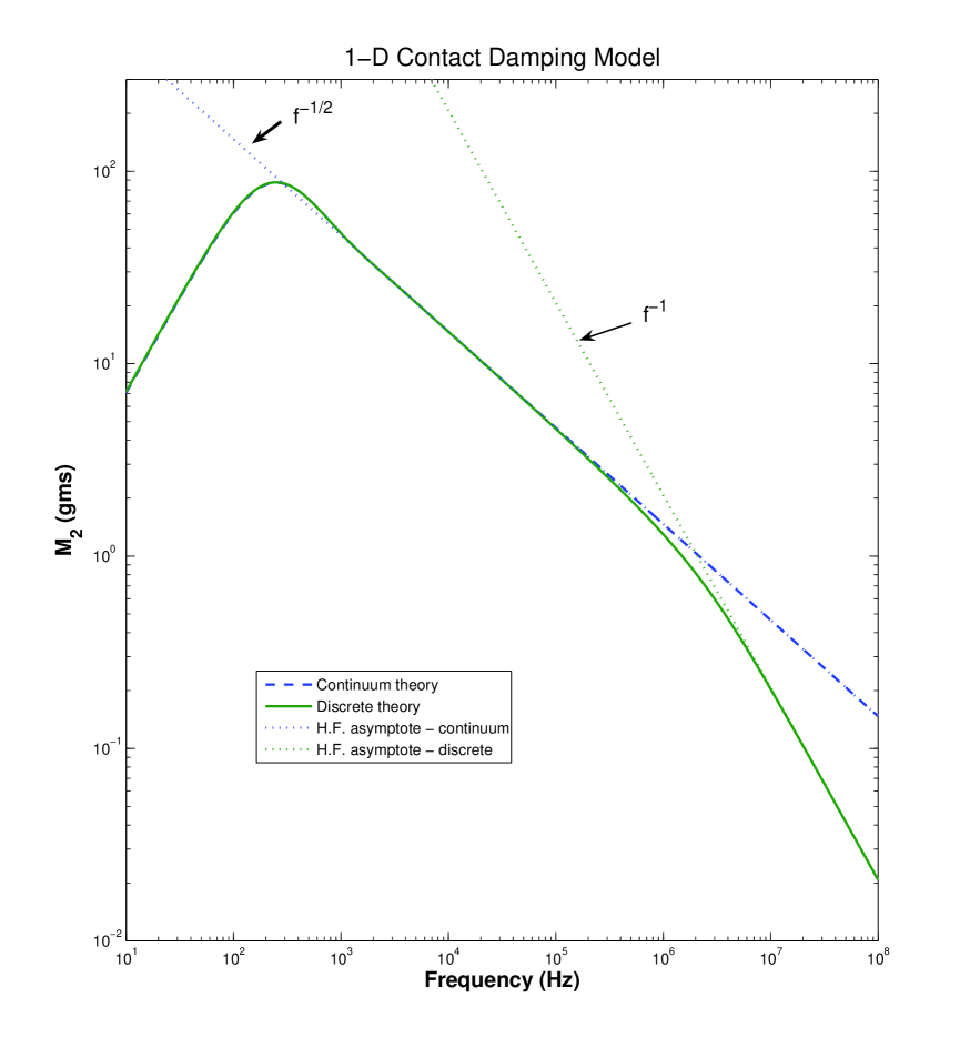
Figure 7: (Color online) Comparison of a continuum versus a discrete theory for a one-dimensional model of local contact dampening. The discrete model closely follows the continuum result except for frequencies high enough such that the macroscopic viscous skin depth becomes smaller than the interparticle separation.

To summarize this Section we may say that there are several distinct possible origins to the frequency dependence of $\tilde{M}$. Within the context of the discrete model, such as embodied in Eqs. (16) and (17), one expects structure near those normal mode frequencies which are relatively near the real axis, as implied by Eq. (22). To the extent that a continuum approximation may be relevant for some of the lower lying modes, one may expect structure when the (wavelength of sound/viscous skin depth) is comparable to the cavity dimensions, examples of which appear in Figures 6a, 6b, or 7. There may be further structure at the frequencies for which the continuum theory breaks down, an example of which is seen around 3 (MHz) in Figure 7. And finally, there may be structure due to the fact that the springs themselves exhibit a non-trivial frequency dependence, an example of which is given by Eq. (20).

V Effective Macroscopic Properties

V.1 Liquids

A wide variety of real liquids satisfies the assumptions of Model I. We have measured $\tilde{M}(\omega)$ for four simple liquids. In Figure 8 we show the results for a common, commercially available, fluorocarbon, whose chemical formula is $N(CF_{3}(CF_{2})_{4})_{3}$. By fitting Eq. (28) to this data, we are able to extract the density, $\rho$, and the speed of sound: $V=\sqrt{K_{0}/\rho}$. These values, measured with our effective-mass technique for all four liquids, are cross-plotted against those determined by more conventional means selfridge ; crc in Figure 9. As there is a good agreement, both for density and for sound speed, we conclude that our technique for measuring the dynamic effective mass $\tilde{M}(\omega)$ is an accurate one.

Figure 8: Real part of the effective mass of a fluorocarbon fluid compared against the theoretical prediction of Eq. (28). The 1/4 wavelength resonance is visible around 6 (kHz).

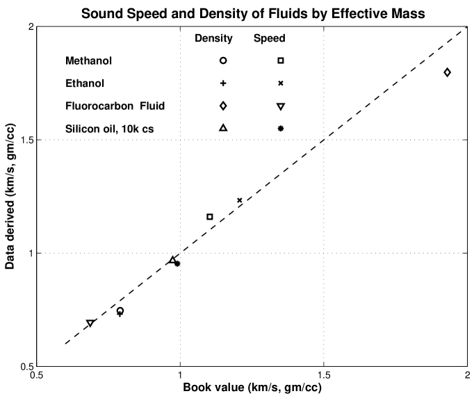
Figure 9: Densities and sound speeds of various liquids measured with our effective mass technique and crossplot against those values determined by more conventional means selfridge ; crc .

V.2 Granular Media

Encouraged by these results, we naively interpret the main resonance in Figures 2 and 5 as being a 1/4 wavelength resonance of the compressional sound speed i.e. analogous to the resonances predicted by Model I. We investigated how this resonance, $f_{g}$, shifts to higher frequencies as the filling depth, $L$, is reduced. Throughout the volume of grains in the cup, the sound speed must be depth dependent; the gravity-attributed stiffness is small at the surface and maximum at the bottom. Nevertheless, we may estimate an effective sound speed in the vertical direction based on this peak frequency and on the filling depth of the tungsten particles:

$$v(L)=4Lf_{g}(L).$$ (37)

Figure 10 shows these estimated speeds as a function of filling level, L, for a cavity with diameter D = 2.54 cm and for cavities of differing diameters, all filled to the same level, L = 3.05 cm. For this figure we have filled the cavities with two different procedures: (1) We vibrate the cavity vertically at 1 (kHz) with different acceleration amplitudes, as indicated. (2) We fill simply by “tapping gently” on the side of the cup. We note that the position of the main resonance in the cup can be very different depending upon the filling technique. Nonetheless, these results show the trend of greater speed with greater depth, as expected. The values we are reporting $\sim$ 100-300 $(m\cdot s^{-2})$ are of the same order of magnitude as those of other granular media reported in the literature using other techniques cremer ; Bourinet2 ; Varanasi_b ; liu ; shield ; schmidt .

In one case shown in Figure 10 we first filled the cup by the vibration measurement and then lightly tapped the side of the cup. This caused the grains to pack less tightly and move the main resonance to a much lower frequency, and thus a much lower apparent sound speed.

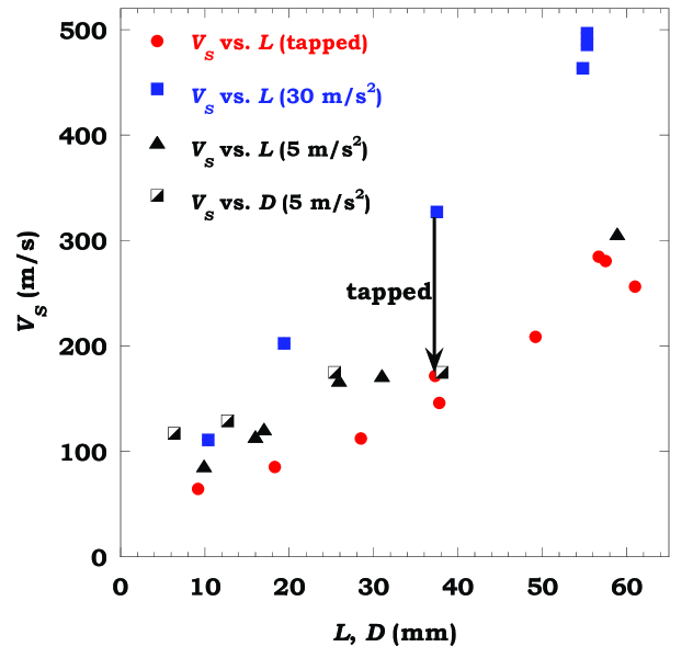
Figure 10: (Color online) Effective speed of sound in tungsten granules as a function of filling depth, L, for constant cavity diameter, D = 2.54 cm , and as a function of cavity diameter, filled to a constant depth, L = 3.05 cm. The numbers in parentheses refer to the maximum amplitude of vibration during the packing protocol.

Also in Figure 10 we show our results for the effective sound speed in cavities of differing diameters, D, filled to a common depth. These data provide evidence of a kind of dynamic Janssen effect in the sense that the side walls support some fraction of the differential force as an effect of the oscillation. In order not to confuse the issue with the dynamic Janssen effect reported previously for that observed in cavities whose walls move at a constant speed bertho , we will refer to the effect in the present paper as the acoustic Janssen effect. If the side walls did not support the effective mass one would expect the effective sound speed to be independent of cavity diameter. We return to this point in our discussions of numerical simulations, below. Suffice it to say that the results of Figure 10 rule out the strict applicability of an interpretation of the main resonance peak based on Eq. (28), Model I: The sound speed is a function of depth and the material has a shear rigidity. This observation, a sound speed in the range 100-300 $(m\cdot s^{-2})$, implies the elastic moduli are in the range $K\sim 1-9\times 10^{7}$ (Pa), which is orders of magnitude smaller than the elastic constants of steel. Therefore, the presence of the granular media in the cavity of the resonance bar contributes negligibly to the stiffening of that bar, as we have assumed.

Because at least some of the effective mass is borne by the side walls of the cavity, we may estimate the effective viscosity of the granular medium based on the high-frequency tail of the data, such as in Figures 2 and 5. According to Model II, the high frequency tail of $\tilde{M}(\omega)$ should be proportional to $\omega^{-1/2}$, as in Eq. (30), when the viscous skin depth is small: $\delta(\omega)\ll a$. Roughly speaking, this is seen in the data plotted in Figure 11. (The data fit better to $f^{-1/2}$ than to $f^{-1}$ although not overwhelmingly so.) Taking into account the prefactors, we conclude that the granular medium has an effective acoustic viscosity $\eta_{\rm eff}=[3-10]\times 10^{4}$ Poise. This value of $\eta_{eff}$ implies a value of the viscous skin depth $\delta(10kHz)\approx 3mm$ which is both small compared to the cup radius and large compared to the grain diameters thus satisfying two of the underlying assumptions in Eq. (30). This value is just an order of magnitude estimate as the fluctuations around the $f^{-1/2}$ behavior are quite large and Model II is, of course, an oversimplification and an overestimation of the effects of the sides of the cavities. It is clear that, while the data exhibit features of both Model I and II, neither model captures the whole story. Nonetheless, if our estimate of the macroscopic viscosity is approximately correct that would imply that the crossover from $M_{2}\propto\omega^{-1/2}$ to $M_{2}\propto\omega^{-1}$ [i. e. Eq. (25)] occurs in the frequency range $[2-8]\times 10^{6}$ (Hz). This crossover happens when the macroscopic viscous skin depth approximately equals the inter-particle separation, $\delta=b$, as discussed in connection with Figure 7. If this crossover happens at all, it would seem to be well outside our experimentally accessible measurement range.

In a similar vein, we may conceptualize the effective elastic constants as $\tilde{K}(\omega)=K_{o}-i\omega\eta$ from which we deduce that a crossover from elastic-dominated to viscous-dominated behavior occurs at a frequency $\omega_{e-v}\sim K_{o}/\eta$ which is approximately 15 (kHz) for the granular systems we have studied. We may very well be seeing this crossover at the higher end of our frequency range in Figure 11.

To summarize this subsection we have found some evidence that there is a an effective macroscopic viscosity in the sense of Eq. (30) being approximately correct. This, in turn, suggests that we should not see behavior implied by Eq. (25) unless the frequency is much higher than we are investigating; we don’t see that behavior, much less that suggested by Eq. (26). Even at our highest frequencies the granular system is undergoing collective oscillation, albeit a complicated one: It is not the case, even at our highest frequency, that only those grains in contact with the walls are contributing to $\tilde{M}(\omega)$.

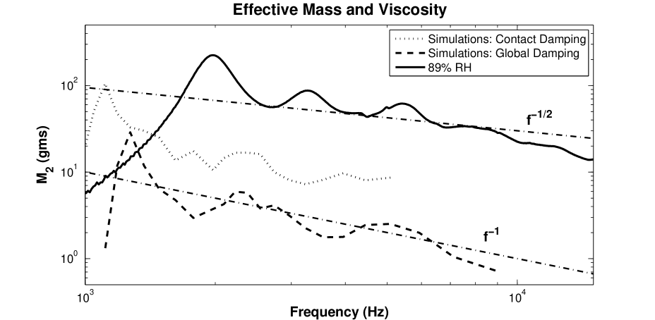
Figure 11: $M_{2}(\omega)$ vs. frequency indicating the possible effect of a macroscopic viscosity in the experimental data. The simulation based on contact dampening is suggestive of a macroscopic viscosity $M_{2}\propto f^{-1/2}$ whereas that based on global dampening $M_{2}\propto f^{-1}$ is not. The simulation results have been shifted vertically.

VI Simulations

The toy models are illuminating as far as they go but to obtain a deeper understanding of the dampening mechanism on a microscopic level we have performed molecular dynamic simulations of $\tilde{M}(\omega)$. Here, we consider the much simpler system of spherical beads confined in a rectangular box.

In our simulations a static packing at a pre-determined pressure is first achieved by methods previously described mgjs , and then we incorporate walls, friction, and the force of gravity. The simulations consider the typical Hertz-Mindlin contact forces for the normal and tangential components, respectively, and the presence of Coulomb friction between the particles characterized by a friction coefficient $\mu$. See Ref. mgjs and references therein for a discussion of the underlying physics of these contact forces.

Microscopic dampening is provided by two principal mechanisms of dissipation: (a) Local dampening, in which the force is proportional to the relative velocity between two contacting grains poschel2 ; wolf-md . Examples of this form of dampening include intrinsic attenuation due to asperity deformation poschel2 , and wetting dynamics within the liquid bridges between adjacent grains as they move relative to each other crassous1 , crassous2 . (b) Global dampening, in which there is a presumed rotational and translational drag due to a viscous fluid, such as air, which is assumed to move with the walls of the cavity. See rayleigh ; thornton ; wolf-md . Within the context of Eqs. (16) and (17) the global dampening approximation is that the particles not in direct contact with the walls still experience a drag effect such that ${\bf K}_{iw}=-i\omega{\bf B_{w}}$, where ${\bf B_{w}}$ is the same for each grain. The conclusions we draw from our numerical simulations are relatively insensitive to the assumed values for the dampening parameters, either global or local. We plot some typical results in Figure 11 where we indeed see that the local dampening hypothesis implies $M_{2}\propto\omega^{-1/2}$ and the global dampening is more consistent with $M_{2}\propto\omega^{-1}$. The data are quite noisy and the distinction between $f^{-1/2}$ and $f^{-1}$ behavior is not clear-cut, although the fit to $f^{-1/2}$ is somewhat better. In Section VII.2 we demonstrate quite unequivocally that contact damping is the operative mechanism in the experimental data.

Results are displayed in Figure 12 for a system in which there is assumed to be only local contact dampening. The two cases shown correspond to normal and transverse contact forces (top) and normal forces only (bottom). The fundamental resonance and the broad high-frequency tail are clearly evident. We show, separately, the contribution to $\tilde{M}(\omega)$ from the bottom as well as from each of the side walls. The conclusions we draw from the numerical modeling are:

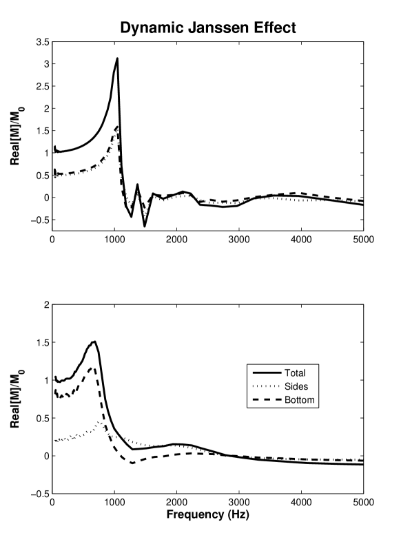
Figure 12: Acoustic Janssen effect as seen in molecular dynamic simulations. The real part of the computed effective mass, normalized to the static mass, is plotted versus frequency: (Top) $\mu=0.5$, (Bottom) $\mu=0$. Although both simulations clearly show the resonance, in the former approximately one-half of the effective mass is supported by the side walls and one-half by the bottom.

1. An acoustic Janssen effect reveals that Models I and II (Section IV.3) are equally important to an understanding of the dynamics. Figure 12a shows the results of the effective mass at the bottom and on the walls of the cavity, as a function of the frequency, for a system with friction coefficient $\mu=0.5$. For all frequencies, we find that approximately one-half of the mass is held by the bottom and the other half by the side walls. In this sense, one cannot make the distinction between the simplified models. Our depiction of an effective sound speed as a function of filling level, Figure 10, is really just a manner of speaking. When the friction is switched off ($\mu=0$, Fig. 12b), almost all the weight is supported by the bottom walls of the cavity, as expected, since the effective shear modulus becomes negligibly small mgjs ; therefore the Model II effect essentially disappears. (A small component of the weight is held by the walls because they are made of glued particles in the simulations.) Not surprisingly, we still see the resonance peaks as predicted by Model I.

We note that our results for the effective sound speed measured in cavities of different diameters but filled to the same depth, plotted in Figure 10, provide an experimental indication of an acoustic Janssen effect. If the side walls did not support the effective mass one would expect the effective sound speed to be independent of cavity diameter.

2. Simulations allow us to differentiate between possible different microscopic origins of dissipation. We find that either global or local dampening can capture the main features of the experiments: the main resonance peak, as in Model I, and a broad background, as in Model II. However, the high-frequency asymptotic behavior for large $\omega$ is very different for the two mechanisms. Global dampening predicts $\tilde{M}(\omega)\sim i\omega^{-1}$, as per Eq. (25) where $B_{iw}$ is nonzero for every particle. Roughly speaking this can be seen in the result plotted in Fig. 11. On the other hand, as long as the viscous skin depth $\sqrt{2\eta_{\rm eff}/\rho\omega}$ is large compared to the grain size but small compared to the cup radius, then contact dampening predicts $\tilde{M}(\omega)\sim(i/\omega)^{1/2}$, as in Model II. This trend is seen in the numerical simulations based on contact dampening plotted in Fig. 11. Although the simulation result is noisy, we may conclude that there is an effective viscosity, as is seen in the experimental results. Contact dampening can be caused by viscoelasticity of the grains themselves or it can be induced by liquid bridges at the contact points ocon ; damour ; crassous1 ; crassous2 . We are inclined to suppose it is the latter that dominates in our samples and this has motivated us to consider the effects of humidity on our results, both for $\tilde{M}(\omega)$ and for the resonances in the bar. We present our results in the next section. For reasons which will become apparent, we need to develop a quantitative theory of the bar resonances that goes beyond the perturbation theory, which we also describe in the next section

VII Detailed Theory of Flex Bar Resonances

The perturbation theory described in Section III is informative but in some situations $\tilde{M}(\omega)$ takes on very large values - larger even than the mass of the bar itself, thus invalidating the assumption that $\tilde{M}(\omega)$ is a small perturbation. Moreover, there are resonances seen in the loaded bar which are primarily resonances within the granules themselves; perturbation theory is not able to make any prediction about these resonances. For situations such as these it is necessary to go beyond the perturbation theory and use a more complete theory. For the case of a rectangular bar the flex mode resonances, including the effect of the granular medium, can be computed directly. This technique is described in Appendices A and B. Basically, the theory treats the bar as a one dimensional object for which flex waves are described by the so-called Timoshenko beam theory timoshenko . The extra compliance near the center of the bar, due to the existence of the cavity, is modeled by a single parameter, $\xi$, whose value is set by the resonance frequency when the cavity is empty. There are no other adjustable parameters. As before, though, we treat the effective mass of the grains $\tilde{M}(\omega)$ as a localized point density.

At each (complex-valued) frequency there are two left-going and two right-going waves. The amplitudes of these four components are determined by the requirement that four homogeneous boundary conditions must be satisfied. The normal-mode condition is that the determinant of these coefficients must vanish; we search, numerically, for the complex-valued normal-mode frequencies, $\{\omega_{R}\}$, at which the determinant vanishes.

We compare the results of this theory, first against resonance bar data taken when the cavity is filled to different depths with various liquids, and then to data taken when the cavity is filled with granular media, under conditions of differing humidity.

VII.1 Liquids

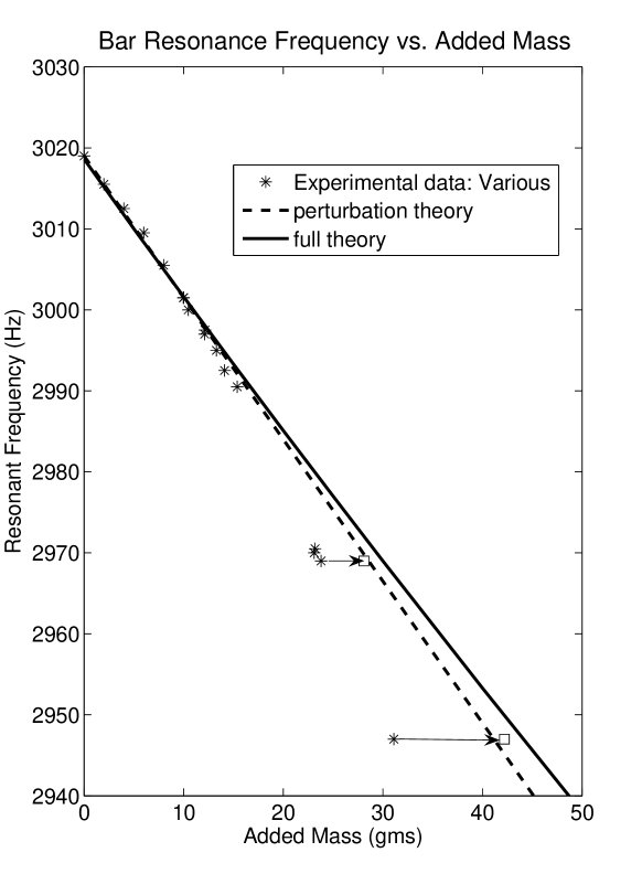
Figure 13: Resonance frequency of steel bar as a function of added mass in the cavity, for various liquids, filled to various depths. The solid curve is the prediction based on the theory described in Appendix A. The dashed curve is the perturbation theory thereof Eq.(7). The two data points indicated with squares represent the effective mass of those liquids evaluated at the resonance frequency, using Eq. (28).

In Section V.1 we showed how the effective mass measurements on simple liquids gave results in general agreement with the predictions of Model I, Eq. (28). It is natural to inquire whether the theory described in Appendix A can accurately predict the frequency shift of a resonant bar whose cavity is filled to varying depths with such a simple liquid. In Figure 13 we show the measured results of the flexural resonance frequency of the bar when the cavity is partially filled with the liquids considered in connection with Figure 9. The solid curve represents the predictions of the theory described in Appendix A, assuming the effective mass within the cavity is frequency independent. Over the range of added mass values, the full theory is nearly the same as the predictions of the perturbation theory, Eq. (7). We have determined $I_{1}\approx 2.1$ for the fundamental mode in our bar, reflecting the fact that the displacement at the center is much larger than the average RMS displacement. For large enough values of added mass the resonance frequency predicted by the full theory asymptotes to a finite frequency, reflecting the fact that even if the center of the bar is pinned, the two arms may still oscillate freely. The difference between the full theory and the perturbation theory is quite large for added masses on the order of 500 grams, which is off the scale of Figure 9. The data mostly lie on the theoretical curve except for the data points greater than 20 g, which correspond to a fluorocarbon fluid. For these data points it is simple enough to estimate $\tilde{M}(\omega)$, evaluated at the measured resonance frequency, using Eq. (28). With this correction to the added mass all the data for the simple fluids now lie nearly on the theoretical curve, which gives us confidence in our approach.

VII.2 Granular Media - Humidity Effect

In order to elucidate the physical origin of the dampening mechanism we have undertaken a controlled study of the effects of humidity on these systems. Both the shaker cup and the resonant bar are filled with the same amount of grains, by weight, of tungsten particles. They are packed into their respective cavities using the mechanical compaction protocol described in Section II.3. Both the shaker apparatus and the resonant bar are placed in a hermetically sealed glove box. The humidity is controlled by placing an open pan of salt-saturated water inside, as well. We have used different salts in the water as a means of controlling the humidity. We use a low power fan to provide a continuous flow of air throughout the container. The temperature is held at T = $26.5^{o}$ C. The glove box sits on a vibration isolation table. The motivation here is to allow for equilibration of humidity on a reasonable time scale and to not allow for extraneous vibrations to dislodge the grains in the cavities.

In Figure 14 we show a comparison of the measured and the computed resonance frequencies in the bar as a function of elapsed time. We also show how the humidity is changing, as we swap one salt-saturated solution for another. (The “zero” humidity cases are accomplished with a desiccant.) There are several different resonance frequencies that were measurable. For each of them we have determined the complex-valued resonance frequency, $\tilde{f_{R}}$, using the procedure described at the end of Section II.2. The width of each resonance is indicated with the error bars. i.e. What is plotted is ${\rm Re}(\tilde{f_{R}})$ and ${\rm Re}(\tilde{f_{R}})\pm{\rm Im}(\tilde{f_{R}})$. Using the simultaneously measured $\tilde{M}(\omega)$ in the shaker cup, we are able to compute the expected (complex-valued) resonance frequencies in the bar, using the theory described in Appendices A and B. These computed resonance frequencies are depicted in the same manner as the measured ones, in Figure 14. The horizontal dashed line is the resonance frequency in the unloaded bar, $f_{0}$. Its Q is so high ($\sim 1000$) that the width (a few Hertz) does not show on the scale of Figure 14; see Figure 3, top. The other dashed curve in Figure 14 plots the position and width of the main resonance frequency seen in $\tilde{M}(\omega)$, $f_{g}$.

A few selected plots of $\tilde{M}(\omega)$ are shown in Figure 15. The main resonance in $\tilde{M}(\omega)$ is clearly visible in Figure 15 but, in fact, there is another resonance of smaller amplitude, around 4500 (Hz) for the 43% and 73% humidity cases, which is barely visible in Figure 15.

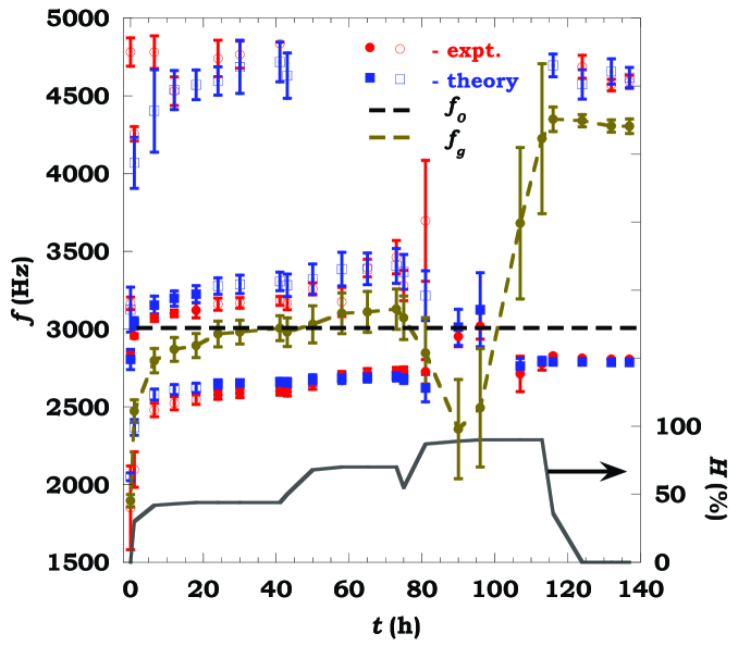
Figure 14: (Color) Comparison of measured and predicted resonant bar characteristics at various humidities. The “error bars” indicate the width of the resonances, as described in the text. The filled symbols refer to the dominant mode in the system, which is predominantly “bar-like”. The horizontal dashed line, $f_{0}$, is the resonance frequency in the unloaded bar. Its Q is so high that the width does not show on the scale of the figure. $f_{g}$ shows the position and width of the main resonance seen in the effective mass data, some of which is show in Figure 15. The solid curve is the relative humidity in the glove box vs. time.

There are several interesting features to the data of these two Figures. First, from either Figure 14 or Figure 15 we see that the position of the main resonance within $\tilde{M}(\omega)$ starts at a low [$\sim 2000$ (Hz)] frequency when the humidity is initially zero. It then increases as the humidity increases to 43% then again to 73%. Concomitantly, the width of that resonance also increases; the system of loose particles is becoming more dampened with increasing humidity. Second, there is generally quite good agreement between theory and experiment as to the position and widths of the several different resonances in Figure 14. Third, although the strongest resonance in the bar around 3 (kHz) dominates, there are also one or two other resonances, which we associate with the dynamics within the granular medium.

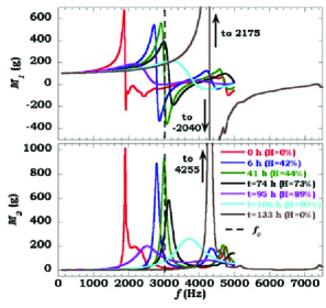
Figure 15: (Color) Evolution of dynamic effective mass as the humidity is changed, as per the humidity data in Figure 14.

We have noticed that, of the two resonances seen in the bar in the region 2000-3500 (Hz), one of them has a significantly larger amplitude than the other, as is clear from the example shown in Figure 3, which corresponds to t = 41 hours in Figures 14 and 15. This “stronger” resonance is labeled with filled symbols, for both the measured and computed resonances, in the legend of Figure 14; the others are labeled with open symbols. Our interpretation is that the two “bare” modes, the resonance in the empty bar at $f_{0}$, and the resonance in $\tilde{M}(\omega)$ at $f_{g}$, have coupled to each other to yield two hybrid modes in the bar + grains system, an upper branch and a lower branch. The resonance with the larger amplitude corresponds to a mode which is predominantly bar-like. When $f_{g}<f_{0}$, at early times, the real part of the effective mass is negative in the vicinity of $f_{0}$. Although the theoretical calculations were done with the complete theory of Appendix A, it is useful to consider the qualitative predictions of the perturbation theory. According to the predictions of Eq. (7), one may expect the resonant frequency in the bar should increase relative to that of the empty bar due to this negative mass loading, and this is just what we see in the upper branch. At slightly later times, when the humidity is increased to $\sim 70\%$, $f_{g}$ has increased above $f_{0}$, with the result that the real part of $\tilde{M}(\omega)$ is now positive, in the region around $f_{0}$. Now, according to the perturbation theory, the resonance frequency in the bar should decrease and this, too, is just what we see. An analogous behavior was seen in the data of Kang et al Kang who considered the behavior of the resonance frequency of a clamped plate as more and more loose beads were placed atop it. Our view of their experiments is that for low values of mass-loading, the resonance frequency, $f_{g}$, in their grains is higher than the resonance frequency of their plate. Thus, the real part of their effective mass is positive and the resonance frequency is initially lowered, relative to the unloaded value. If the depth of loading is large enough, $f_{g}$ drops below the plate resonance frequency and the real part of $\tilde{M}(\omega)$ can become negative. This is our explanation of why the observed resonance frequency may then increase, relative to the unloaded value.

Although the frequency of the upper branch in Figure 14 is relatively slowly varying, it very abruptly changes character, from “bar-like”, at the early times, to “grain-like” later. The lower branch shows the opposite behavior. This aspect of the response of the system will be analyzed in detail elsewhere Valenza .

When the system is at 90% humidity, it behaves quite differently. (There is an initial drop in humidity which is an artifact of our procedure for swapping in and out the salt-saturated solutions.) The main resonance in $\tilde{M}(\omega)$ initially drops to around 2200 (Hz) but, more significantly, it becomes very much broadened relative to that at the lower humidities, cf. Figure 15. We do not understand the initial drop in the resonance frequency; conceivably it is related to the initial drop in humidity. At this humidity, we were able to locate only one resonance in the experimental bar data and we were also able to locate only one in the theoretical computations. As time goes on, maintaining the humidity in the glove box constant, we see from Figures 14 and 15 that the main resonance in $\tilde{M}(\omega)$ increases with time. It increases with time for the lower humidities, too, though it is most pronounced for 90% humidity. Previously Hsu , we analyzed this aspect of the data in the context of an assumed distribution of asperity heights within the contact region. With time more and more of the energetically favorable asperity regions become filled with condensate, assuming they are smaller than the Kelvin radius, Eq.(38), below. Under a fairly broad set of assumptions, this lead to the prediction that the contact stiffnesses would increase approximately logarithmic in time, which is what was observed. The data sets analyzed in Reference Hsu were, however, prepared using the vibration protocol described earlier in Section II.3, unlike the data in Figures 14 and 15. Nonetheless, we believe that this is what is happening: At any given level of humidity, there is a relatively slow process of equilibration leading to a relatively slow increase in the resonance frequency within $\tilde{M}(\omega)$.

Finally, when the salt solution is replaced with a desiccant, causing the humidity to drop to essentially zero, there is a very dramatic change in the properties of the granular medium. According to Figure 15 the main resonance has shifted up to a very high frequency, $\sim 4300$ (Hz). It has become extremely sharp, and extremely strong. Concurrently, in the bar there are two distinct resonances, the one primarily within the grains, around 4500 (Hz), and the other primarily in the bar, around 2800 (Hz). We note that both of these are significantly sharper (higher Q) resonances than their counterparts in the humid stages. We note that theory and experiment are in general agreement as to the level of attenuation of the various modes. Specifically, the attenuation of the bar resonance [$\sim 3000$ (Hz)] is much reduced in the dried out state relative to that in the humid states.

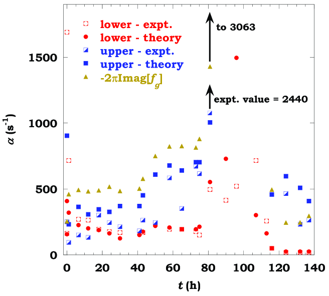
Figure 16: (Color) Decay rate, $\alpha\equiv-{\rm Im}\omega_{R}$, of the various normal modes depicted in Figure 14. Here, “upper” and “lower” refer to the two branches with resonance frequency near 3 (kHz).

We don’t really know why we see two resonances in the dry cases and one, two, or three in the humid cases, depending, but this seems to be the situation both for the theory and the experiment. In the theory, for 90% humidity, one may speculate that there is an additional resonance or resonances, presumably related to the apparent resonance seen in Figure 15, but that it/they appear for very large values of the dampening rate i.e. well off the real axis. However, if they exist we have been unable to locate such resonances with our theoretical machinery no matter what value we use for seeding the mode search, as described in Appendix A.

In order to analyze the effectiveness of the granular medium in attenuating the modes in the bar, at the various humidities, we re-plot part of the data of Figure 14 in Figure 16. Here, $\alpha\equiv\;{\rm Im}[\omega_{R}]$ represents the decay rate of the amplitude, $A$, of each mode, in the time domain, viz: $A\propto e^{-\alpha t}$. We are quite pleased with the general level of agreement between theory and experiment, the exceptions occurring when the system is still equilibrating to humidity changes, from 80 to 110 hours. We note also that the agreement is generally better for the “bar-like” mode than it is for the “grain-like” mode. The decay rate of the unloaded bar is so small, $\alpha$(unloaded) = 9.4 $(neper\cdot s^{-1})$, that it appears to be zero on the scale of Figure 16. We see from the Figure that there is a monotonic effect of humidity on the decay rate of the main resonance within the granular medium, as shown in gold. Such is not the case for the dampening coefficient of the mode which is predominantly bar-like in the combined system. Even though the humidity varies from 43% to 70% in the first 80 hours, the measured dampening rate of this mode exhibits only a small, non-systematic, variation. This variation is, however, captured in the theory. At $t=80$ hours, when the humidity is raised to 90%, the measured and the predicted dampening rates of this mode both increase enormously. When the salt-saturated solution is replaced with a desiccant the measured and computed dampening rates drop to very small values, much smaller than when the system was originally in the dry state. (We note that the grains in the shaker cup seem to equilibrate with humidity changes more rapidly than do the grains in the bar, but eventually they tend to the same state. Perhaps this is a consequence of the different flow patterns of air in the vicinity of the two cavities in the glove box.)

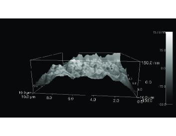
Figure 17: AFM image of the surface texture of a tungsten granule showing asperities on the 10-20 nm scale. Note the differing vertical and horizontal scales.

Our observed humidity effect is very much analogous to that seen in the results of D’Amour et al. damour who deduced very similar behavior from their measurements of the changes in resonance behavior of a quartz plate whose top surface was covered with a monolayer of beads. They concluded that the in situ drying of the contacts between the beads and the quartz causes them to stick over a larger microscopic surface area, causing the asperities on the surfaces in the contact zone to be partially crushed. This, in turn, causes the stiffness of the contact “springs” to increase and the dampening to decrease. A rough analogy would be when one soaks tissue paper with water it is easy to make it stick to a vertical surface; the mess is held up by the force of surface tension. If it is allowed to dry, the force of adhesion to the wall actually increases, even though the water is gone. That is because as it dries it also deforms, allowing a large area of solid-on-solid contact to develop. This, basically, is what we see in our own measurements. An AFM image of the surface of one of the tungsten granules in Figure 17 shows these asperities on the scale of 10-20 nm. Capillary condensation within these asperities occurs when the Kelvin radius, $r_{m}$, is approximately equal to the asperity size where

$$r_{m}=-\frac{2\gamma V_{L}}{RT\ln(H)}\>=-\frac{1.04\>{\rm nm}}{\ln(H)}\>\>\>,$$ (38)

where $\gamma$ is the liquid vapor surface tension, $R$ is the gas constant, $T$ is the absolute temperature, $V_{L}$ is the molar volume, and $H$ is the relative humidity GreggSing . The numerical value in the second equation is that which is appropriate to water at $26.5^{o}$ C. Thus, at a relative humidity of 90% the Kelvin radius is approximately 10 nm, which is large enough that a single liquid bridge engulfs all the asperities in the contact region between neighboring particles.

We conclude, therefore, that the dominant mechanism of acoustic dampening in granular media is due to the adsorbed film of water which exists on the particles, an example of contact dampening. In particular, the film in the region between two contacting grains undergoes a shear deformation due to the relative motion of the two grains and thus it gives rise to dampening due to the viscosity of the water in the film. Conceptually this may be thought of as an example of the “squirt mechanism” squirt which is operative as the dominant attenuation mechanisms in sedimentary rocks at ultrasonic frequencies. In that case there is clear evidence that the pore fluid is squeezed in and out of microscopic cracks which exist within the cement material holding the grains together.

The data in Figure 16, especially the low attenuation in the second dry state, clearly rule out global dampening or intrinsic dampening within the Tungsten as being significant mechanisms for dampening.

It is also clear from Figures 14 and 15 that the adsorbed films of water at the grain-grain contacts is a significant mechanism for stiffness of the inter-granular spring constants. However, the sound speed data in Figure 10 indicate that something like a Hertz-Mindlin contact forces must also be operative: Why else would the effective sounds speeds be dependent upon the cavity dimensions? Because of the odd shape of our tungsten granules it is difficult to analyze the relative contributions to the grain-grain stiffness due to each of these mechanisms. For the simpler geometry of a random close packing of spherical glass beads it is possible to do this estimate, precisely because of the data of D’Amour et al. damour on a monolayer of beads lying on a vibrating quartz substrate. From their published data, their Figure 1 and Equation (5), it is simple enough to estimate the strength of the spring constants ($\kappa$ in their notation, not to be confused with our use of $\kappa$ in our Eq. 29) between the beads and the quartz plate. We find, from their data,

$$\kappa({\rm Single\>Bead:\>Exp.})=[1-7]\times 10^{4}\>({\rm N\cdot m^{-1}})\>\>\>,$$ (39)

depending upon the humidity, in their experiments. These values are much larger than what one might expect for Hertz contact theory in which the weight of the bead provides a static compression and subsequent stiffness of the contact. Equations (1-8) of Norris and Johnson NJ in which the normal force, N, is the weight of a glass bead, gives

$$\kappa({\rm Single\>Bead:\>Hertz})=4.6\times 10^{3}\>({\rm N\cdot m^{-1}})\>\>\>.$$ (40)

In doing this estimate we assumed the relevant radius of the contact is the radius of the bead itself, 100 $\mu$m; had we assumed a radius equal to that of a typical asperity on the surface of the bead, the computed stiffness would be orders of magnitude smaller than Eq. (40). This estimate is further confirmation of the conclusions of D’Amour et al. damour , that the stiffness of the contacts is due to surface forces. If, however, one considers the contact stiffness of glass beads at a depth of 2.54 cm, compressed by the weight of the beads above, one may estimate the expected stiffness predicted by Hertz contact theory to be

$$\kappa({\rm Hertz\>at\>Depth})=2\times 10^{4}\>({\rm N\cdot m^{-1}})\>\>\>.$$ (41)

Thus, we may say that the contact stiffness for grains near the top surface of a granular-filled cavity - virtually any granular-filled cavity - is due to humidity mediated surface forces. However, for those grains a few centimeters deep Hertz-Mindlin contact theory is also important.

We conclude this subsection by pointing out that the measurement technique of D’Amour et al damour is very much analogous to our measurements on the flex bar. In both cases one is looking at changes in the resonance frequency of some system due to the, relatively small, perturbation of the granular medium. In addition our measurements of $\tilde{M}(\omega)$ represent a more direct measurement of the underlying physics of the granular medium. In this regard the humidity effect on $\tilde{M}(\omega)$ is quite strikingly apparent, over a wide frequency range as shown in Figs. 14 and 15. Although the dampening factor for the bar under humid conditions is much greater than that dry, the differences in the main bar resonance are not nearly so great as in the effective mass itself.

VIII Conclusions

We have shown how a measurement of the frequency-dependent effective mass of a granular aggregate, $\tilde{M}(\omega)$, allows us to predict, accurately, the effects of a grain-filled cavity on the acoustic properties of a resonant structure. This fact gives us a more direct access to an investigation of the underlying physical mechanisms relevant to the dampening effect of granular media on structure-borne sound. Crudely speaking, we may think of these systems as having an effective speed of sound (small) and an effective viscosity (large). The dissipation mechanism occurs at the grain-grain contact level as our simulations have indicated and our humidity controlled experiments have made unavoidably clear. As the humidity is increased there is a large increase in the attenuation of the fundamental resonance within the grains, Im($f_{g}$), which translates to a non-monotonic, but calculable, variation in the attenuation of the structural resonance in the bar, Im($f_{R}$). When the system is taken to a high level of humidity, and then dried to the same level of humidity as it was at the beginning, there is a dramatic reduction in attenuation and a dramatic increase in stiffness of the grain-grain contacts, at the end of this humid-dry cycle relative to that in the initial dry state. We understand this effect in terms of increased solid-on-solid contact area at the grain-grain contacts.

Appendix A: Treatment of Bar Resonances Using Timoshenko Theory

The very simple one dimensional theory of wave propagation in a flexing bar Kinsler is not accurate enough for a quantitative treatment of the effect of a granular effective mass on the frequency shift and change of quality factor. Basically this is because the ratio of length to thickness of our bar is not large enough (the frequency is not low enough). Accordingly we start with the more sophisticated, but still one-dimensional, theory developed by Timoshenko timoshenko . The equation of motion for the vertical displacement is

$$\begin{array}[]{l}EI\frac{\partial^{4}u}{\partial x^{4}}+\rho A\frac{\partial^{2}u}{\partial t^{2}}\\ \\ -\rho I\left(\frac{E}{k\mu}+1\right)\frac{\partial^{4}u}{\partial x^{2}\partial t^{2}}+\frac{\rho^{2}I}{k\mu}\frac{\partial^{4}u}{\partial t^{4}}=0\>\>\>\>,\end{array}$$ (A-1)

where $E$ is the Young’s modulus, $A=wd$ is the cross-sectional area of the bar in terms of its thickness, $w$, and depth, $d$. $\rho$ is the density of the bar and $\mu$ is the shear modulus. $\rho I$ is the moment of inertia of the cross-section of the bar relative to its mid-point: $I=(1/12)w^{2}A$ for a rectangular bar. $k$ is a shape parameter which we take to be equal to (8/9) as is appropriate for a bar of rectangular cross-section. The simple theory for a flexing bar corresponds to keeping only the first two terms on the LHS of Eq. (A-1).

At each frequency, which is in general complex-valued, the solution can be written as a linear combination of four linearly independent solutions:

$$\begin{array}[]{l}u=[A\sin(q_{1}x)+B\cos(q_{1}x)\\ \\ +C\sinh(q_{2}x)+D\cosh(q_{2}x)]e^{-i\omega t}\end{array}\>\>\>,$$ (A-2)

where $q_{1,2}(\omega)$ are determined by a direct substitution of Eq. (A-2) into Eq. (A-1). Because we are interested only in the fundamental mode, which is symmetric w.r.t. $x=0$, we need only consider the region $0<x<L/2$. The coefficients $[A,B,C,D]$ are determined by the requirement that certain boundary conditions be satisfied at the ends on the bars, $x=\pm L/2$, and at the center, $x=0$. However, the coefficients $A$ and $C$ are not equal to zero, as we shall see, due to the fact that the slope, $\frac{\partial u}{\partial x}$, is not continuous at $x=0$.

As we discuss in the main text, we assume the dynamic effective mass is located at the point $x=0$ and we are treating the bar as effectively a one-dimensional object. Taking into account the missing mass of steel in the cavity the density is

$$\rho({x})=\rho_{0}+\frac{\tilde{M}(\omega)-M_{h}}{A}\delta({x})$$ (A-3)

where $\rho_{0}$ is the density of steel, $M_{h}=\rho_{0}\pi a^{2}L$ is the missing mass of steel taken from the cavity, and $A$ is the cross-sectional area of the bar. One of the boundary conditions is that the net force exerted by the bar on the cavity must equal the net mass times the acceleration, viz:

$$\begin{array}[]{ccl}-[\tilde{M}(\omega)-M_{h}]\omega^{2}u(0)&=&-[F(0^{+})-F(0^{-})]\\ &&\\ &=&-2F(0^{+})\end{array}$$ (A-4)

where $F(x)$ is the force which the bar exerts on the element $x^{+}$. Within the context of Timoshenko theory, it is specified in terms of specific spatial and temporal time derivatives of $u(x)$ timoshenko . Thus Eq. (A-4) gives one of the four necessary boundary conditions on the coefficients $[A,B,C,D]$.

The presence of the cavity at $x=0$ makes this region of the bar very bendable. The radius of curvature in this region is very much smaller than it is away from the cavity. We model this effect as if the left and right halves of the bar are hinged together such that the bending angle between the two halves is proportional to the bending moment imposed by the bar:

$$\frac{\partial u}{\partial x}\mid_{0^{+}}=\xi\tau(0^{+})\>\>\>,$$ (A-5)

where $\tau(x)$, the bending moment, is also given in terms of spatial and temporal derivatives of $u(x)$. The parameter $\xi$ characterizes the “bendableness” of the cavity region. $\xi=0\leftrightarrow\frac{\partial u}{\partial x}\mid_{0^{+}}=0$ corresponds to no additional extra compliance, whereas $\xi\rightarrow\infty\leftrightarrow\tau(0^{+})=0$ corresponds to a completely flexible hinge. We determine the numerical value of $\xi$ by the requirement that the measured and computed resonance frequency of the bar with an empty cavity, $\tilde{M}\equiv 0$, must match. It is the only free parameter in the theory.

The remaining two boundary conditions are that both the force and the bending moment vanish at the end of the bar:

$$F(L/2)=0$$ (A-6)

and

$$\tau(L/2)=0\>\>\>.$$ (A-7)

.

There are, therefore, four homogeneous linear equations in the four unknowns ${\bf X}=[A,B,C,D]$ i.e. $H_{ij}X_{j}=0$ and so the determinant of the matrix of coefficients must vanish for any non-trivial solution. We search for such complex-valued roots, $\omega_{R}$, such that det$[H(\omega_{R})]=0$ using Muller’s method numrec . In general there is a countably infinite number of such normal mode solutions. One must choose a set of three initial frequencies with which the algorithm initiates the search. Generally, we have chosen the three to be of the form [0.95, 1.00, 1.05]$\omega_{S}$, where the seed frequency, $\omega_{S}$, may be complex-valued. The normal mode frequency to which the algorithm converges, if any, depends upon the value of $\omega_{S}$ that is chosen. In the case of the data shown in Figure 14 the value of the seed frequency needed to be very close to the resonances around 4 (kHz), but did not need to be very close to the ones found near 3 (kHz).

As a check, we have compared the theory vs. experiment for a similar steel bar having no cavity at all: $\tilde{M}\equiv M_{h}$ and $\xi\equiv 0$. The dimensions of this bar are L X W X D = 20.32 X 3.05 X 3.81 cm and we used parameters $\rho=7830\;(kg\cdot m^{-3})$, $V_{c}=5800\;(m\cdot s^{-1})$ and $V_{s}=3100\;(m\cdot s^{-1})$ which we have measured ourselves on the steel samples. There are two directions in which this bar can flex; we measured and we computed the fundamental resonance frequency for each orientation. The results are shown in Table 1. We see that the predictions of the full theory agree with the measured values, to within a few tenths of a percent (better than the accuracy with which the input parameters are known), whereas the predictions of the simple flex theory differ by as much as 10%. The accuracy of the former approach is more than acceptable for our purposes whereas that of the latter is not.

Table 1: Comparison of measured and predicted resonance frequencies for a bar with no cavity (Hz).

	Measured	Full Theory	Simple Theory
Flex Horiz.	3542	3529	3793
Flex Vert.	4272	4260	4741

In order to implement the theory when the cavity is filled with a granular medium we need a means to compute $\tilde{M}(\omega)$ for complex-valued $\omega$, though the input data is limited to real-valued $\omega$. We describe how to do this in Appendix B.

Appendix B: Analytic Continuation of $\tilde{M}(\omega)$ for Complex Values of $\omega$.

Figure 18: (Color online) Test of rational function approximation. The symbols represent the value of the function, Eq. (B-1), for values of $z$ on the real axis. These 20 values are used to construct a rational function approximation for arbitrary complex-values $z$. It is compared against the original function for $z=x-0.095i$ where we see that there is a near perfect overlay of the two functions.

With the shaker apparatus we have determined the dynamic effective mass for a series of real-valued frequencies: $\tilde{M}(\omega_{j})\>\>j=1,\cdots,N$. In order to use this information for purposes of computing the resonance frequency in the flexing bar, as described in Appendix A, we need to be able to evaluate $\tilde{M}(\omega)$ for arbitrary complex values of $\omega$. This is because the normal mode frequency of the bar will be complex-valued, reflecting the attenuation in the system. We have chosen to do this analytic continuation using the rational function technique, a Bulirsch-Stoer algorithm, as described in Reference numrec . In essence, the algorithm approximates the function as a ratio of two polynomials - a rational function. The algorithm has the property that the rational function passes through each input datum exactly. Thus, any noise in the input data does propagate. In order to test how well this approach actually does the analytic continuation, we consider the following simple function:

$$F(z)=-\left\{\frac{1}{\sin[z-(5-i))]}+\frac{2}{\sin[z-(7-0.1i)]}\right\}\>\>\>.$$ (B-1)

We have evaluated this function for 20 different real values of $z$, and these values are plotted in Figure 18.

With these 20 values we construct the rational function approximation and plot it for values of $z$ on a line in the complex plane parallel to the x-axis: $z=x-0.095i$. We also plot Eq. (B-1) on the same graph where we see that the rational function basically overlays the actual function, even for values of $z$ near one of the poles. In fact, the difference between the two never exceeds 1%. This test gives us confidence to use the rational function to analytically continue $\tilde{M}(\omega)$ into the complex $\omega$-plane.

References

- (1) W. Kuhl and H. Kaiser, Acustica 2, 179 (1962).
- (2) L. Cremer and M. Heckl, Structure Borne Sound (Springer, Berlin, 1973).
- (3) J. M. Bourinet and D. Le Houèdec, Computers and Structures 73, 395 (1999).
- (4) J. M. Bourinet and D. Le Houèdec, Powders & Grains 97 ed. R. Behringer and J. Jenkins Balkema, Rotterdam, 1997.
- (5) G. Kurtze, VDI-Berichte 8, 110 (1956).
- (6) C.-J. Hsu, D. L. Johnson, R. A. Ingale, J.J. Valenza, N. Gland, and H.A. Makse, Phys. Rev. Lett. 102, 058001 (2009).
- (7) J. C. Sun, H. B. Sun, L. C. Chow, and E. J. Richards, J. Sound and Vibration 104, 243 (1986).
- (8) S. A. Nayfeh, J. M. Verdirame, and K. K. Varanasi, Proc SPIE 4697, 158 (2002)
- (9) K. K. Varanasi and S. A. Nayfeh, Proc DETC’03 ASME Design Emg. Tech. Conf. (2003).
- (10) W. Kang, J. A. Turner, F. Bobaru, L. Yang, and K. Rattanadit, J. Acoust. Soc. Am. 121, 888 (2006).
- (11) B. R. Tittmann, V. A. Clark, and J. M. Richardson, J. Geophys. Res. 85, 5199 (1980).
- (12) Th. Brunet, X. Jia, and P. Mills, Phys. Rev. Lett. 101, 138001 (2008).
- (13) L. E. Kinsler and A. E. Frey, Fundamentals of Acoustics (Wiley, New York, 1950).
- (14) J. B. Mehl, J. Acoust. Soc. Am. 64, 1523 (1978); M. B. Ewing and J. P. M. Trusler, J. Acoust. Soc. Am. 85, 1780 (1989).
- (15) W. H. Press, B. P. Flannery, S. A. Teukolsky, and W. T. Vetterling, Numerical Recipes, (Cambridge University Press, New York, 1987).
- (16) J. B. Knight, C. G. Fandrich, C. N. Lau, H. M. Jaeger, and S. R. Nagel, Phys. Rev. E 51, 3957 (1995); E. R. Nowak, J. B. Knight, M. L. Povinelli, H. M. Jaeger, and S. R. Nagel, Powd. Tech. 94, 79 (1997); E. R. Nowak, J. B. Knight, E. Ben-Naim, H. M. Jaeger, and S. R. Nagel, Phys. Rev. E 57, 1971 (1998); J. Brujic, P. Wang, C. Song, D. L. Johnson, O. Sindt, and H. A. Makse, Phys. Rev. Lett. 95, 128001 (2005).
- (17) L. D. Landau and E. M. Lifshitz, Electrodynamics of Continuous Media (Pergamon, NY, 1960); L. D. Landau and E. M. Lifshitz, Statistical Physics 2nd ed. (Addison-Wesley, Reading, 1969).
- (18) L. D. Landau and E. M. Lifshitz, Fluid Dynamics (Pergamon, NY, 1978).
- (19) D. L. Johnson and P. N. Sen, Phys. Rev. B 24, 2486 (1981); D. L. Johnson, J. Koplik, and R. Dashen, J. Fluid Mech. 176, 379 (1987).
- (20) M. J. Turner, I. M. MacLeod, and A. D. Rothberg, J. Appl. Physiol. 67, 472 (1989).
- (21) A. Selfridge, IEEE Trans. Sonics and Ultrasonics 32 (1985).
- (22) Handbook of Chemistry and Physics, 81st Edition (CRC Press, Cleveland, 2000).
- (23) C.H. Liu and S. R. Nagel, Phys. Rev. Lett. 68, 2301 (1992); C.H. Liu and S. R. Nagel, Phys. Rev. B 48, 15646 (1993).
- (24) F. D. Shields, J. M. Sabatier and M. Wang, J. Acoust. Soc. Am. 108, 1998 (2000).
- (25) H. Schmidt, Acustica 4, 639 (1954).
- (26) Y. Bertho, F. Giorgiutti-Dauphine, and J.-P. Hulin, Phys. Rev. Lett. 90, 144301 (2003).
- (27) H. A. Makse, N. Gland, D. L. Johnson, and L. M. Schwartz, Phys. Rev. E 70, 061302 (2004).
- (28) N. V. Brilliantov, F. Spahn, J.-M. Hertzsch, and T. Pöschel, Phys. Rev E 53, 5382 (1996).
- (29) J. Schäfer, S. Dippel, and D. E. Wolf, J. Phys. I (France) 6, 5 (1996).
- (30) J. Crassous, E. Charlaix, and J.-L. Loubet, Phys. Rev. Lett. 78, 2425 (1997).
- (31) J. Crassous, E. Charlaix, H. Gayvallet, and J.-L. Loubet, Langmuir 9, 1995 (1993).
- (32) Lord Rayleigh, Theory of Sound, (Dover Publications, New York, 1945 edition, 1877).
- (33) C. Thornton, and D. J. Barnes, Acta Mechanica 64, 45 (1986).
- (34) R. J. O’Connell and B. Budiansky, J. Geophys. Res. 79, 5412 (1974).
- (35) J. N. D’Amour, J. J. R. Stålgren, K. K. Kanazawa, C. W. Frank, M. Rodahl, and D. Johannsmann, Phys. Rev. Lett. 96, 058301 (2006).
- (36) S. Timoshenko and D. H. Young, Vibration Problems in Engineering, 3rd ed., (van Nostrand, Princeton, 1955).
- (37) J. Valenza and D. L. Johnson (unpublished).
- (38) S. J. Gregg and K. S. W. Sing, Adsorption, Surface Area and Porosity 2nd. ed. (Academic, New York, 1982).
- (39) W. M. Murphy, K. W. Winkler, and R. L. Kleinberg, Geophysics 51, 757 (1986).
- (40) A. N. Norris and D. L. Johnson, J. Appl. Mech. 64, 39 (1997).