Asymptotics-based CI models for atoms: properties, exact solution of a minimal model for Li to Ne, and application to atomic spectra

Abstract

Configuration-Interaction (CI) models are approximations to the electronic Schrödinger equation which are widely used for numerical electronic structure calculations in quantum chemistry. Based on our recent closed-form asymptotic results for the full atomic Schrödinger equation in the limit of fixed electron number and large nuclear charge [FG09], we introduce a class of CI models for atoms which reproduce, at fixed finite model dimension, the correct Schrödinger eigenvalues and eigenstates in this limit.

We solve exactly the ensuing minimal model for the second period atoms, Li to Ne. The energy levels and eigenstates are in remarkably good agreement with experimental data (comparable to that of much larger scale numerical simulations in the literature), and facilitate a mathematical understanding of various spectral, chemical and physical properties of small atoms.

1 Introduction

From the early days of quantum mechanics it has been clear that the chemical behaviour of atoms and molecules is governed by their energy levels and electron configurations, which in turn are determined, to very high accuracy, by the eigenvalues and eigenstates of the Schrödinger equation $H\psi=E\psi$. But 80 years on, high-accuracy numerical computation of such data remains a largely unresolved challenge, even for the smallest of systems such as a single Carbon atom. The only computations of which we are aware which meet the mathematical ideal [BLWW04] of convergence tables showing an increasing number of converged digits as a function of basis set size or number of iteration steps (for a reproducibly documented algorithm for the original problem) concern two-electron systems such as He and H₂. See [KNN08] for recent advances and references.

The underlying reasons are two-fold.

First, a “curse of dimension” phenomenon is present: the Schrödinger equation for an atom or molecule with $N$ electrons is a partial differential equation in ${\mathbb{R}}^{3N}$, so direct discretization of each coordinate direction into $K$ gridpoints yields $K^{3N}$ gridpoints. Thus the Schrödinger equation for a single Carbon atom ($N=6$) on a ten point grid in each direction ($K=10$) already has a prohibitive $10^{18}$ degrees of freedom.

Second, one is dealing with a tough multiscale problem: chemical behaviour is not governed by total energies, but by small energy differences between competing states. Even for very small systems, these are typically several orders of magnitude smaller than total energies. For instance, as shown in the table below, the spectral gap between ground state and first excited state of the second period atoms is less than 1 $\%$ of the total size of these energy levels in all cases, and only about 0.1 $\%$ for Carbon, Nitrogen and Oxygen. Nevertheless this tiny gap is of crucial importance, as the two states it separates have different spin and angular momentum symmetry, and hence completely different chemical behaviour.

Atom	Li	Be	B	C	N	O	F	Ne
$\begin{array}[]{l}\mbox{\small Ratio of first spectral gap}\\ \mbox{\small to ground state energy}\end{array}$	0.0093	0.0068	0.0053	0.0012	0.0016	0.00096	0.0078	0.0047

Table 1: Multiscale structure of atomic spectra (experiment, [RJK⁺07]).

To deal with the curse of dimension, in quantum chemistry a large array of reduced models has been developed. For small systems with up to one or two dozen electrons, the most accurate and most widely used class of models are the Configuration-Interaction (CI) models, whose origins go back to the early years of quantum mechanics (see e.g. [Hyl29]) and whose systematic development started with the work of Boys [Boy50] and Löwdin [Loe55]. Roughly speaking, these are “tensor product Galerkin approximations”: the full electronic Schrödinger equation is projected onto a subspace spanned by carefully chosen Slater determinants (= antisymmetrized tensor products), which are in turn formed from a small set of orbitals (= elements of the single-particle Hilbert space $L^{2}({\mathbb{R}}^{3}\times{\mathbb{Z}}_{2})$).

Different CI models differ by the choice of orbitals and the selection of the subset of Slater determinants. The question of how to best make these choices remains the subject of a great deal of current research in the quantum chemistry literature, with the best methods to date relying on a combination of chemical intuition, computational experience, and nonlinear parameter optimization, as well as on a huge number (between 10⁶ and 10⁹) of included determinants. See [SO96, HJO00] for a general overview of the CI method and its most common variants such as Doubly excited CI (DCI), Multi-determinant Hartree-Fock (MDHF), Complete active space self-consistent field method (CASSCF), Coupled-Cluster theory (CC), and the (desirable but usually not practical) Full CI (FCI), and see e.g. [BT86, TTST94, KR02, BM04, CNMCJ05, Joh05, NNKI07, KNN08] for applications to atomic energy level calculations.

Our goal in this paper is to introduce, analyze, and apply to atomic energy level prediction a particular class of CI models for atoms which exploit our recent closed-form asymptotic results for the full atomic Schrödinger equation in the limit of fixed electron number $N$ and large nuclear charge $Z$ [FG09]. Namely, we require that the model of fixed finite subspace dimension $K$ reproduce correctly the first $K$ Schrödinger eigenvalues and eigenstates in this limit.

That such a requirement can be met by a fixed-resolution CI model is not trivial (for example, it is not met by Hartree-Fock theory, even in an infinite, complete one-electron basis), but a simple consequence of the asymptotic results in [FG09] (see Section 2.4).

The above limit exhibits the important multiscale effect that the ratio shown experimentally in Table 1 of first spectral gap $\Delta E$ to ground state energy $E$ of the Schrödinger equation tends to zero [FG09]. The requirement that the corresponding eigenstates and gaps be nevertheless captured correctly by an approximation should hence be relevant to yielding good eigenstates and gaps in the realistic situation when this ratio is small.

In fact, even the minimal asymptotically correct CI model for atoms and ions with 1 to 10 electrons (eq. (A’), (B’), (C’) in Section 2.4), whose subspace dimension turns out to be 8, 28, 56, 70, 56, 28, 8 for Li, Be, B, C, N, F, turns out to be very interesting.

• We find that the requirement of asymptotic correctness leads to Slater orbitals $P(x)e^{-\gamma|x|}$ (where $P$ is a polynomial and $\gamma>0$ a constant), not Gaussian orbitals $P(x)e^{-\gamma|x|^{2}}$ used in the overwhelming majority of numerical CI computations on account of their easy facilitation of two-centre integral evaluation. See Section 2.4.

• The model is exactly soluble (via the methods introduced in [FG09]), except for the determination of the dilation parameters $\gamma$ in the Slater orbitals, which are straightforward to calculate numerically with very high accuracy. See Section 3.

• The model does remarkably well when compared to experimental data and high-dimensional simulations in the literature. It captures around 99 percent of the ground state energy in all cases, without a single empirical parameter! See Figure 1. Moreover the predicted ground state spin and angular momentum quantum numbers (¹S for He, Be, Ne, ²S for H and Li, ⁴S for N, ²P for B and F, and ³P for C and O) come out right in each case; spectral gaps are captured well (and in a significant number of cases more accurately than in the benchmark numerical multi-determinant Hartree-Fock calculations of Tatewaki et al [TTST94] which used a much larger basis set); and for $N\geq 5$ the model is never outperformed by more than a factor ten by any method, including large-scale simulations with subspace dimension bigger than $10^{7}$. For a detailed comparison see Section 4.

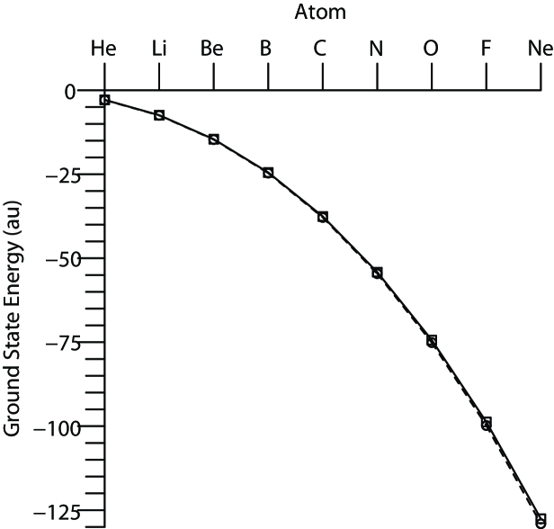
Figure 1: Experimental (dashed) and minimal asymptotics-based CI (solid) ground state energies of atoms.

Thus, our work yields for the first time few-parameter, explicit, closed-form approximations to the low-lying eigenstates of the atoms Li, Be, B, C, N, O, F, Ne which are of chemically relevant accuracy. These provide a hopefully useful reference for the calibration of numerical methods, and a valuable tool to advance mathematical understanding of physical, chemical and spectral differences between the elements. For example, the ground state wavefunctions confirm the basic mathematical picture of the periodic table obtained in [FG09] by asymptotic analysis of the Schrödinger equation for strongly positive ions, and make it quantitative for neutral atoms; and they allow to trace the size of spectral gaps to individual Coulomb and exchange integrals, thereby making more rigorous longstanding insights by quantum chemists and revealing the cancellations that lead to the small size of gaps compared to total energies (Table 1). See Section 4.

Nevertheless a great many open problems remain, even for minimal asymptotics-based CI.

1) In this paper we demonstrate its accuracy via comparing to experimental values (see Section 4) and proving desirable theoretical properties (see Section 2), but how can it be understood in terms of rigorous error estimates comparing it to the Schrödinger equation?

2) In particular, why is the use of just one dilation parameter per one-electron subspace $V_{j}$ so effective? As far as we are aware, although screening parameters are widely used (see Section 2), there are no rigorous mathematical results regarding their effectiveness. For instance, one might hope such parameters to emerge in some order expansion of a suitably scaled problem.

3) How does the model fare for larger atoms? For this step we would suggest automation of the calculation of the eigenspaces and energy expressions (analogous to Tables 2–3), and Fourier transforms and one- and two-body integrals (as in Lemmas 3.1 and 3.2). We would hope the model to show interesting chemical effects such as the shell ordering $4s<3d$, and its occasional reversal, in the transition metals.

Finally, it is highly desirable that the asymptotics-based CI approach introduced here be extended to molecular problems. The principal observation (Theorem 2.1 (ii)) that CI models of fixed finite subspace dimension can be constructed which reproduce correctly the first K Schrödinger eigenvalues in a large nuclear charge limit is not limited to atoms, as will be discussed elsewhere. But in the molecular case the ensuing orbitals are not available in closed form, and hence do not lead so readily to a mathematical picture of basic physical and chemical properties.

2 Asymptotics-based CI models for atoms

2.1 General CI models

We begin with a mathematical description of CI methods. We find it convenient to do so in the more abstract setting of subspaces and subspace projections rather than the, equivalent, setting of basis sets and expansion coefficients used in the chemistry literature [SO96]. Moreover we introduce a rigorous distinction between general and symmetry-preserving CI methods. (Both of these, as well as hybrid methods in which the solution to a non-symmetry-preserving model is projected a posteriori onto an invariant subspace, are in use in the chemistry literature.)

Starting point for the derivation of any CI model is the exact (nonrelativistic, Born-Oppenheimer) time-independent Schrödinger equation for atoms and ions which one seeks to approximate,

$$H\Psi=E\Psi,$$ (1)

where, for nuclear charge $Z>0$ and $N$ electrons and in atomic units,

$$H=\underbrace{\sum_{i=1}^{N}\Big{(}-\frac{1}{2}\Delta_{x_{i}}-\frac{Z}{|x_{i}|}\Big{)}}_{=:H_{0}}+\underbrace{\sum_{1\leq i<j\leq N}\frac{1}{|x_{i}-x_{j}|}}_{=:V_{ee}},$$ (2)

$E\in{\mathbb{R}}$, and

$$\Psi\in L^{2}_{a}\big{(}({\mathbb{R}}^{3}\times{\mathbb{Z}}_{2})^{N}\big{)}.$$ (3)

Here and below the $x_{i}\in{\mathbb{R}}^{3}$ are electronic position coordinates, $s_{i}\in{\mathbb{Z}}_{2}=\{\pm\frac{1}{2}\}$ are spin coordinates, and $L^{2}_{a}$ is the usual Hilbert space of $N$-electron functions $\Psi\,:\,({\mathbb{R}}^{3}\times{\mathbb{Z}}_{2})^{N}\to{\mathbb{C}}$ which are square-integrable,

$$\int_{{\mathbb{R}}^{3N}}\sum_{({\mathbb{Z}}_{2})^{N}}|\Psi(x_{1},s_{1},\dots,x_{N},s_{N})|^{2}=||\Psi||^{2}<\infty,$$ (4)

and satisfy the antisymmetry principle that, for all $i$ and $j$,

$$\Psi(\dots,x_{i},s_{i},\dots,x_{j},s_{j},\dots)=-\Psi(\dots,x_{j},s_{j},\dots,x_{i},s_{i},\dots).$$ (5)

Mathematically, $H$ is a bounded below, self-adjoint operator with domain $L^{2}_{a}\cap H^{2}$, where $H^{2}$ is the usual Sobolev space of $L^{2}$ functions with second weak derivatives belonging to $L^{2}$. It is known that for neutral atoms ($Z=N$) and positive ions ($Z>N$), there exists an infinite number of discrete eigenvalues, the corresponding eigenspaces being finite-dimensional (Zhislin’s theorem, see [Fri03] for a short proof).
Translating [SO96] into mathematical terminology, a CI model is a tensor product Galerkin approximation to the many-electron Schrödinger equation. More precisely:
Definition 2.1 A CI model of an $N$-electron system with Hamiltonian $H$ is a projection of the Schrödinger equation (1) of form

$$PHP\Psi=E\Psi,\;\;\;\Psi\in V,\;\mbox{$V$ a subspace of $L^{2}_{a}$},\;P=\mbox{projector onto $V$},$$ (6)

with the additional requirement that $V$ must possess a basis consisting of Slater determinants.
Recall that a Slater determinant is an anti-symmetrized tensor product $|\eta_{1}\dots\eta_{N}\rangle\in L^{2}(({\mathbb{R}}^{3}\times{\mathbb{Z}}_{2})^{N})$ of orthonormal one-electron functions $\eta_{i}\in L^{2}({\mathbb{R}}^{3}\times{\mathbb{Z}}_{2})$, the antisymmetrization being necessary to comply with the quantum mechanical law (5). The difference between different CI models lies in the freedom to choose the subspace $V$, or – in quantum chemistry language – to select a set of orbitals and a set of Slater determinants to be included into the CI expansion.

Note that if $V$ is spanned by the orthonormal Slater determinants $\Psi_{\alpha}$, $\alpha=1,\dots,M$, the projection operator $P$ onto $V$ has the expansion $\sum_{\alpha=1}^{M}|\Psi_{\alpha}\rangle\langle\Psi_{\alpha}|$, and eq. (6) can be written in its more standard matrix form $Ac=Ec$, where $A$ is the M$\times$M matrix with entries $A_{\alpha\beta}=\langle\Psi_{\alpha}|H|\Psi_{\beta}\rangle$, and $c$ is the coefficient vector in the expansion $\Psi=\sum_{\alpha}c_{\alpha}\Psi_{\alpha}$. The more abstract form (6) emphasizes the elementary fact that the CI eigenvalues and eigenstates only depend on the subspace $V$, not on the choice of basis within this subspace.
A basic desirable feature of CI models, not related to the tensor product structure but only to that of a linear subspace projection, is the following.

Lemma 2.1.

(Rigorous upper bound) For $j=1,\dots,\mbox{dim}\,V$, we have $E_{j}\leq E^{CI}_{j}$, where $E_{j}$ and $E_{j}^{CI}$ are the $j^{th}$ eigenvalue, including multiplicity, of the Schrödinger equation (1) respectively the CI equation (6).

Proof This is an immediate consequence of the min-max theorem for discrete eigenvalues of a self-adjoint operator below the bottom of the essential spectrum [RS78].

2.2 A mathematical definition of the notion of configuration for atoms

In the quantum chemistry literature, the word “configuration” is often employed as a synonym for Slater determinant [SO96]. But in the atomic physics and atomic spectroscopy literature (e.g. [RJK⁺07]), as well as some of the best computational studies, the word “configuration” has a more subtle meaning, which takes into account the important role played by spin and angular momentum symmetries. For our mathematical purposes, the latter notion turns out to be very useful, so let us formalize it mathematically.

First, recall the total angular momentum operator ${\bf\underline{L}}=(L_{1},L_{2},L_{3})$, the total spin operator ${\bf\underline{S}}=(S_{1},S_{2},S_{3})$ and the parity operator $\hat{R}$, along with the fact that the operators

$${\bf\underline{L}}^{2},{\bf\underline{S}}^{2},L_{3},S_{3}\text{ and }\hat{R}$$ (7)

commute with each other and with $H$ (see [FG09] for the result, as well as a mathematical definition of the operators ${\bf\underline{L}}$, ${\bf\underline{S}}$ and (7)).

One starts from a finite number of mutually orthogonal subspaces of the single-electron Hilbert space,

$$V_{1},...,V_{k}\subset L^{2}({\mathbb{R}}^{3}\times{\mathbb{Z}}_{2}),$$ (8)

which are irreducible representation spaces for the joint spin and angular momentum algebra $Span\,\{L_{1},L_{2},L_{3},S_{1},S_{2},S_{3}\}$. In elementary terms, this means that the subspaces must be of “fixed angular and spin symmetry” and “minimal dimension”, more precisely: each $V_{i}$ must be invariant under the $L_{i}$ and $S_{i}$, the operators ${\bf\underline{L}}^{2}$ and ${\bf\underline{S}}^{2}$ must be constant on $V_{i}$, and $V_{i}$ must have minimal dimension (i.e. dimension $(2s+1)(2\ell+1)|_{s=1/2}=2\cdot(2\ell+1)$ when ${\bf\underline{L}}^{2}=\ell(\ell+1)I$ and ${\bf\underline{S}}^{2}=s(s+1)I$; note that the spin quantum number $s$ equals $1/2$ for any $V_{i}$, since ${\bf\underline{S}}^{2}=\frac{3}{4}I$ on the whole single-electron state space $L^{2}({\mathbb{R}}^{3}\times{\mathbb{Z}}_{2})$).
Definition 2.2 A configuration of an $N$-electron atom or ion is a subspace of N-electron state space (3) of the following form:

$$\mathcal{C}^{d_{1},..,d_{k}}=\,\mbox{Span}\,\Bigl{\{}|\chi_{1},\dots,\chi_{N}\rangle\,\Bigl{|}\Bigr{.}\,\{\chi_{1},\ldots,\chi_{N}\}\mbox{ any ON set with }\sharp\{i\,|\,\chi_{i}\in V_{j}\}=d_{j}\Bigr{\}},$$ (9)

where $V_{1},..,V_{k}\subset L^{2}({\mathbb{R}}^{3}\times{\mathbb{Z}}_{2})$ are mutually orthogonal irreducible representation spaces of the joint spin and angular momentum algebra, and $d_{1},...,d_{k}$ is a partition of $N$ (i.e. $d_{j}\in{\mathbb{N}}\cup\{0\}$, $\sum_{j}d_{j}=N$).
The main point here is that all choices of the $\chi_{i}$’s consistent with the requirement that a fixed number of them have to be picked from each $V_{j}$ have to be included.

As an elementary but important consequence, each configuration is invariant under the spin and angular momentum operators ${\bf\underline{L}}$ and ${\bf\underline{S}}$, and in particular under the operators (7). This is immediate from the invariance of the $V_{i}$ under ${\bf\underline{L}}$ and ${\bf\underline{S}}$ and the following identity for the application of one-body operators to Slater determinants: $\sum_{j=1}^{N}A(j)|\chi_{1}\cdots\chi_{N}\rangle=\sum_{j=1}^{N}|\chi_{1}\cdots(A\chi_{j})\cdots\chi_{N}\rangle$.
Example 1: The configurations $1s^{2}2s$ and $1s^{2}2p$ for Lithium.
Let

$$V_{1} =\,\mbox{Span}\,\{\phi_{1s}\!\uparrow,\,\phi_{1s}\!\downarrow\},\;\;\;V_{2}=\,\mbox{Span}\,\{\phi_{2s}\!\uparrow,\,\phi_{2s}\!\downarrow\},$$

$$V_{3} =\,\mbox{Span}\,\{\phi_{2p_{i}}\!\uparrow,\,\phi_{2p_{i}}\!\downarrow\;|\;i=1,2,3\},$$ (10)

where the $\phi$’s are the hydrogen-like orbitals

$$\phi_{1s}(x) :=\frac{Z_{1}^{3/2}}{\sqrt{\pi}}e^{-Z_{1}|x|}$$

$$\phi_{2s}(x) :=\left(\tfrac{3Z_{2}^{5}}{8\pi(4Z_{1}^{2}-2Z_{1}Z_{2}+Z_{2}^{2})}\right)^{1/2}\left(1-\tfrac{1}{6}(2Z_{1}+Z_{2})|x|\right)e^{-Z_{2}|x|/2}$$ (11)

$$\phi_{2p_{i}}(x) :=\frac{Z_{3}^{5/2}}{\sqrt{32\pi}}x_{i}e^{-Z_{3}|x|/2},\;i=1,2,3,$$

$Z_{1}$, $Z_{2}$, $Z_{3}$ are positive parameters, and $\uparrow$, $\downarrow$ denote the spin functions $\uparrow(s)=\delta_{\frac{1}{2}}(s)$, $\downarrow(s)=\delta_{-\frac{1}{2}}(s)$.

Note that the orbitals in (10) are orthonormal (hence the coefficients in $\phi_{2s}$), and that for $Z_{1}=Z_{2}=Z_{3}=Z$ they reduce to the standard eigenstates of the hydrogen atom Hamiltonian $-\frac{1}{2}\Delta-\frac{Z}{|x|}$. The $Z_{i}$ will play an important role later.

For $N=3$, choosing the partitions $d_{1}=2$, $d_{2}=1$, $d_{3}=0$ respectively $d_{1}=2$, $d_{2}=0$, $d_{3}=1$ yields the subspaces (or configurations)

$$\mathcal{C}^{2,1,0} =\,\mbox{Span}\,\{|\phi_{1s}\!\uparrow,\,\phi_{1s}\!\downarrow,\,\phi_{2s}\!\uparrow\rangle,\;|\phi_{1s}\!\uparrow,\,\phi_{1s}\!\downarrow,\,\phi_{2s}\!\downarrow\rangle\},$$

$$\mathcal{C}^{2,0,1} =\,\mbox{Span}\,\{|\phi_{1s}\!\uparrow,\,\phi_{1s}\!\downarrow,\,\phi_{2p_{i}}\!\uparrow\rangle,\;|\phi_{1s}\!\uparrow,\,\phi_{1s}\!\downarrow,\,\phi_{2p_{i}}\!\downarrow\rangle\;|\;i=1,2,3\}.$$ (12)

We call these subspaces 1s²2s¹ and 1s²2p¹. In chemistry this terminology is common to describe the structure of individual wavefunctions, but in the setting just introduced, it is independent of which wavefunction is chosen.

For $Z_{1}=Z_{2}=Z_{3}=Z$, these subspaces have the interesting physical meaning that they are the bottom two eigenspaces of the Lithium atom Hamiltonian in first order perturbation theory [FG09].
Example 2: The subspace $2p_{1}^{1}2p_{2}^{1}$ for Helium
The subspace

$$\tilde{C}=\,\mbox{Span}\,\{|\phi_{2p_{1}}\!\uparrow,\phi_{2p_{2}}\!\downarrow\rangle,\;|\phi_{2p_{1}}\!\downarrow,\phi_{2p_{2}}\!\uparrow\rangle,|\phi_{2p_{1}}\!\uparrow,\phi_{2p_{2}}\!\uparrow\rangle,\;|\phi_{2p_{1}}\!\downarrow,\phi_{2p_{2}}\!\downarrow\rangle\}$$

is not a configuration, because the selection of Slater determinants does not correspond to the rule in Definition 2.1. Indeed this subspace is not invariant under the spin and angular momentum algebra. For instance, applying $L_{3}$ to the first Slater determinant gives $i(|\phi_{2p_{1}}\!\uparrow\phi_{2p_{1}}\!\downarrow\rangle-|\phi_{2p_{2}}\!\uparrow\phi_{2p_{2}}\!\downarrow\rangle)$, which lies outside the subspace.

2.3 Symmetry-preserving CI models

A general class of symmetry-preserving CI models can now be defined mathematically. We remark that the principle of symmetry-preserving numerical schemes has proved very successful in other areas of scientific computing, a prime example being symplectic schemes in Hamiltonian dynamics [LR05].
Definition 2.3 A symmetry-preserving CI model for an $N$-electron atom or ion with Hamiltonian $H$ is a finite-dimensional projection of the Schrödinger equation (1),

$$PHP\Psi=E\Psi,\;\;\;\Psi\in V,\;\;\;\mbox{$V$ a subspace of $L^{2}_{a}$},\;\mbox{$P$=orthogonal projector onto }V,$$ (13)

with the additional requirement that

$$V=\,\mbox{Span}\,\{\mathcal{C}^{(1)},\dots,\mathcal{C}^{(K)}\},$$ (14)

where $V_{1},..,V_{k}\subset L^{2}({\mathbb{R}}^{3}\times{\mathbb{Z}}_{2})$ is a collection of mutually orthogonal irreducible representation spaces of the spin and angular momentum algebra, and each $\mathcal{C}^{(j)}$ is a configuration with respect to the $V_{i}$.
Example Taking $V=\,\mbox{Span}\,\{\mathcal{C}^{2,1,0},\,\mathcal{C}^{2,0,1}\}=\,\mbox{Span}\,\{1s^{2}2s,\,1s^{2}2p\}$ (with notation as in Example 1) yields an invariant CI model for Lithium.
The fundamental point of Definition 2.3 is that unlike general CI, symmetry-preserving CI retains the spin and angular momentum symmetries of the atomic Schrödinger equation. In particular, eigenspaces retain well defined spin and angular momentum quantum numbers $S$ and $L$ (see [FG09] for their mathematical definition):

Lemma 2.2.

(Symmetry preservation) For arbitrary $N$ and $Z$, and any invariant CI model (13), (14) as in Definition 2.3, The operators (7)
(i) leave $V$ invariant
(ii) commute with the CI Hamiltonian $PHP\,:\,V\to V$.
In particular, any eigenspace of an invariant CI model possesses a basis of joint eigenstates of the operators (7).

Proof This is an elementary consequence of the invariance of individual configurations under ${\bf\underline{L}}$, ${\bf\underline{S}}$ and $\hat{R}$. Note that the underlying one-electron subspaces $V_{i}$, being ${\bf\underline{L}}^{2}$ eigenspaces with some eigenvalue $\ell(\ell+1)$, are automatically $\hat{R}$ eigenspaces, with eigenvalue $(-1)^{\ell-1}$.
We note the well known fact that the physically important property (i) is violated by standard approximations such as the Hartree-Fock approximation, even when the individual orbitals have well defined spin and angular momentum quantum numbers. For instance, the Slater determinant $|\phi_{2p_{1}}\!\uparrow\phi_{2p_{2}}\!\downarrow\rangle$ is neither an ${\bf\underline{L}}^{2}$ nor an ${\bf\underline{S}}^{2}$ eigenstate.

2.4 Asymptotics-based subspace selection

We now come to the, in applications crucial, issue of selecting a “good” CI subspace $V$ in the approximation (6).

Commonly, this relies on a great amount of chemical intuition, computational experience, and nonlinear optimization. For example, one would employ the set of Slater determinants formed from the first $N+k$ eigenstates of the nonlinear Hartree-Fock equations of the system under consideration (“k-fold excited CI”), solved numerically in a background subspace of dimension $L>>N+k$ spanned by Gaussian orbitals. For more information, common variants and refinements see [SO96, HJO00].

We propose here an alternative strategy, in which the intermediate step of a Hartree-Fock calculation no longer appears, and which is based on three reasonable theoretical requirements. The CI model should

• preserve the symmetry of the atomic Schödinger equation under spatial and spin rotation (see Definition 2.3)

• preserve the virial theorem, i.e. eigenstates should have the correct virial ratio of $-2$ between potential and kinetic energy

• be asymptotically correct in the iso-electronic limit $Z\to\infty$.

By 3. we mean that the model (if its dimension is $K$) reproduces correctly the first $K$ Schrödinger eigenvalues and eigenstates in this limit (see Theorem 2.1 for a precise statement). Note that the limit of large $Z$ captures the physical environment of inner shell electrons in large atoms. Also, recall its important theoretical feature that the ratio of first spectral gap to ground state energy of the Schrödinger equation (1)–(3) tends to zero [FG09], the experimental ratio for true atoms being very close to zero (see Table 1).

We now apply requirements 1, 2, 3 to the atoms Li to Ne, by not designing a largest such model which can be handled computationally, but a minimum-dimensional model. Below, $(Z_{1},Z_{2},Z_{3})=:\underline{Z}$ denotes the vector of dilation parameters appearing in the orbitals (11). We first discuss the case of the ground state. The ensuing minimal CI model for Li, Be, B, C, N, O, F, Ne ground states is then:

(A)	(Choice of a parametrized, asymptotically exact family of subspaces)
	$V(\underline{Z}):=\mbox{Span}\{\mathcal{C}^{2,0,N-2},\mathcal{C}^{2,1,N-3},\mathcal{C}^{2,2,N-4}\}$,
	with the $\mathcal{C}$’s as in (9) and $V_{1},V_{2},V_{3}$ as in (10), (11),
(B)	(Subspace eigenvalue problem)
	$E^{CI}(\underline{Z}):=\mbox{lowest eigenvalue of }P(\underline{Z})HP(\underline{Z})\mbox{ on }V(\underline{Z})$,
	$\Psi^{CI}(\underline{Z}):=\mbox{corresponding normalized eigenstate}$,
	$\mbox{where }P(\underline{Z})=\mbox{orthogonal projector of }L^{2}_{a}(({\mathbb{R}}^{3}\times{\mathbb{Z}}_{2})^{N})\mbox{ onto }V(\underline{Z})$
(C)	(Variational parameter determination)
	$\underline{Z}_{*}:=\mbox{argmin}_{\underline{Z}}E^{CI}(\underline{Z}),\;E^{CI}:=E^{CI}(\underline{Z}_{*}),\;\Psi^{CI}:=\Psi^{CI}(\underline{Z}_{*})$

(In (A), it is understood that only configurations $\mathcal{C}^{d_{1},d_{2},d_{3}}$ for which each $d_{i}$ is $\geq 0$ are included.)

Some remarks are in order.

(1) This model is certainly not the only conceivable model which satisfies 1., 2., 3., especially since condition 3. is only asymptotic, but it is probably the simplest. The subspace $V(\underline{Z})$ in (A) comes from the theorem in [FG09] that the above subspace with $Z_{1}=Z_{2}=Z_{3}=Z$ is asymptotically equal to the union of the lowest eigenspaces of the full Schrödinger equation (1). In particular, this theorem dictates that the $V_{i}$ should consist of Slater orbitals, not the commonly used Gaussian orbitals. The presence of the variable dilation parameters $Z_{i}$ and eq. (C) comes from requirement 2., which is equivalent to stationarity of the energy $\langle\Psi|H|\Psi\rangle$ of eigenstates with respect to dilations (see the proof of Theorem 2.1).

(2) There is no empirical parameter.

(3) The model has the following variational formulation:

$$E^{CI}=\min_{\underline{Z}\in(0,\infty)^{3}}\min_{\Psi\in V(\underline{Z}),\,||\Psi||=1}\langle\Psi|H|\Psi\rangle,$$

with the set of minimizers $\Psi$ being equal to the set of normalized lowest eigenstates of (B). This is an immediate consequence of (C) and the Rayleigh-Ritz variational principle for the bottom eigenvalue in (B).

(4) Dilation parameters like the $Z_{i}$ are closely related to physical ideas of screening, and go back at least to Slater (in the context of the Hartree equations, [Sla30, Sla64]). They are widely used in the quantum chemistry literature, and are in most studies determined a priori, e.g. via a Hartree-Fock calculation (see [BT86, SO96]). However, from a mathematical standpoint it is of interest to determine them variationally for each eigenstate, as done here; this implies that the ensuing wavefunctions satisfy the virial theorem (see Theorem 2.1). Note also that validity of the latter cannot be guaranteed by linear parameters (i.e., subspace enlargement), but requires making the model nonlinear. This is because the dilation group $\Psi\mapsto Z^{3N/2}\Psi(Z\cdot)$, which underlies the virial theorem, is a non-compact group which – unlike the compact groups $SO(3)$ and $SU(2)$ corresponding to angular momentum and spin – leaves no finite-dimensional subspace of $L^{2}_{anti}(({\mathbb{R}}^{3}\times{\mathbb{Z}}_{2}))$ invariant. The proof of this fact is left to the interested reader.
We now extend (B), (C) to excited states. The simplest generalization would be to compute all eigenvalues $E_{j}(\underline{Z})$ and corresponding orthonormal eigenstates $\Psi_{j}(\underline{Z})$ of $P(\underline{Z})HP(\underline{Z})$, then minimize each eigenvalue over $\underline{Z}$.

But this procedure does not maintain the basic property of the full Hamiltonian (2) that eigenstates with different eigenvalue are orthogonal. However, the symmetries described in Lemma 2.2 come to our help. If two eigenstates of the CI Hamiltonian are also simultaneous eigenstates of the operators (7), which we can assume by Lemma 2.2, then they remain orthogonal after minimization of their eigenvalues over the $Z_{i}$, as long as the eigenvalue of at least one of the operators (7) are different. Thus, in each symmetry subspace (i.e., each joint eigenstate of the operators (7)) we determine the values of the $Z_{i}$ that yield the minimum value for the lowest eigenvalue in the subspace, then use this value to calculate all eigenvalues and eigenstates in the subspace. This way, orthogonality is maintained and in particular the CI energy levels remain rigorous upper bounds to the true energy levels. In practice this method is very close to minimization of each eigenvalue, since most symmetry subspaces turn out to be one-dimensional, and none are more than two-dimensional (see the next section). The use of the $Z_{i}$’s from the lower state is of course a somewhat arbitrary choice; it ensures the greatest accuracy possible for the lower lying states (known as “state-specific” method), an alternative would be to choose the $Z_{i}$ so as to solve a least squares problem and minimize the overall error.

To summarize, the minimal CI model for Li, Be, B, C, N, O, F, Ne excited states is as follows. Below, $V^{L,S,P}(\underline{Z})$ denotes the symmetry subspace $\{\Psi\in V(\underline{Z})\,|\,{\bf\underline{L}}^{2}\Psi=L(L+1)\Psi,\,{\bf\underline{S}}^{2}\Psi=S(S+1)\Psi,\,\hat{R}\Psi=p\Psi\}$, where $L$ is a non-negative integer, $S$ a non-negative half-integer, and $p=\pm 1$.

(A’)	(Choice of a parametrized, asymptotically exact family of subspaces)
	As in (A)
(B’)	(Subspace eigenvalue problem) For each symmetry subspace $V^{L,S,p}(\underline{Z})\subset V(\underline{Z})$
	$E^{CI}_{j}(\underline{Z}):=\mbox{eigenvalues of }P(\underline{Z})HP(\underline{Z})\mbox{ on }V^{L,S,p}(\underline{Z})$,
	$\Psi^{CI}_{j}(\underline{Z}):=\mbox{corresponding orthonormal eigenstates}$,
	$\mbox{where }P(\underline{Z})=\mbox{orthogonal projector of }L^{2}_{a}(({\mathbb{R}}^{3}\times{\mathbb{Z}}_{2})^{N})\mbox{ onto }V(\underline{Z})$
(C’)	(Variational parameter determination) For each symmetry subspace $V^{L,S,p}(\underline{Z})\subset V(\underline{Z})$
	$\underline{Z}_{*}:=\mbox{argmin}_{\underline{Z}}(\min_{j}E^{CI}_{j}(\underline{Z})),\;E^{CI}_{j}:=E^{CI}_{j}(\underline{Z}_{*}),\;\Psi^{CI}_{j}:=\Psi^{CI}_{j}(\underline{Z}_{*})$

Let us summarize the additional properties of the model (A’), (B’), (C’) beyond those of general symmetry-preserving CI (Lemmas 2.1, 2.2) in a theorem.

Theorem 2.1.

Let $N\in\{3,..,10\}$, $Z\geq N$. The minimal CI model (A’), (B’), (C’) has the following properties.
(i) (Virial theorem) Any lowest normalized eigenstate $\Psi^{CI}$ of the model in a symmetry subspace (i.e., a joint eigenspace of the symmetry operators ${\bf\underline{L}}^{2}$, ${\bf\underline{S}}^{2}$, $\hat{R}$) satisfies

$$\langle\Psi^{CI}|V|\Psi^{CI}\rangle=-2\langle\Psi^{CI}|T|\Psi^{CI}\rangle,$$

where $T$, $V$ are the kinetic respectively potential part of the Hamiltonian (2).
(ii) (Correct asymptotic behaviour) For $N$ fixed and $Z\to\infty$,

$$\lim\frac{E^{CI}_{j}}{E_{j}}=1,\;\;\;\lim\frac{\Delta E_{j}^{CI}}{\Delta E_{j}}=1,\;\;\;\lim|||P^{CI}_{j}-P_{j}|||=0,$$

where $E^{CI}_{1}<\dots<E^{CI}_{m}$ and $E_{1}<\dots<E_{m}$ are the CI eigenvalues respectively the lowest eigenvalues of the Schrödinger equation (1), $\Delta E^{CI}$ and $\Delta E_{j}$ are the spectral gaps $E^{CI}_{j}-E^{CI}_{1}$ and $E_{j}-E_{1}$ ($j\geq 2$), $P^{CI}_{j}$, $P_{j}$ denote the projectors onto the corresponding eigenspaces, and $|||\cdot|||$ is the operator norm on the $N$-electron Hilbert space $L^{2}_{a}(({\mathbb{R}}^{3}\times{\mathbb{Z}}_{2})^{N})$.

Proof (i) follows from the fact that the manifold $\cup_{\underline{Z}\in(0,\infty)^{3}}V^{L,S,p}(\underline{Z})$ is invariant under dilations $\Psi\mapsto\Psi_{\lambda}(x_{1},s_{1},..,x_{N},s_{N})=\lambda^{3N/2}\Psi(\lambda x_{1},s_{1},..,\lambda x_{N},s_{N})$, $\lambda>0$, which makes the usual proof of the virial theorem applicable: normalized minimizers $\Psi$ of $\langle\Psi_{\lambda}|H|\Psi_{\lambda}\rangle$ in this manifold satisfy $0=\frac{d}{d\lambda}\Big{|}_{\lambda=1}\langle\Psi_{\lambda}|H|\Psi_{\lambda}\rangle$.

(ii) is a consequence of the asymptotic results in [FG09] together with the elementary inequalities $E_{j}\leq E^{CI}_{j}\leq E^{PT}_{j}$, where the $E^{PT}_{j}$ are the lowest eigenvalues of the PT model [FG09].
We remark that statement (ii) fails when the Slater orbitals (11) are replaced by finite linear combinations of Gaussians, or indeed by any functional form which fails to reproduce (11) asymptotically [FG09].

It is instructive to compare the above argument in favour of Slater orbitals to the well known Kato cusp condition argument. Theorem 2.1 (ii) concerns the limit $N$ and $x$ general, $Z\to\infty$, whereas the asymptotic regime of the Kato cusp condition is $N$ and $Z$ general, $x\to 0$; the latter is therefore insufficient to specify whole orbitals, as it only concerns their behaviour at $x=0$.
Finally, let us formulate a hierarchy of higher and higher dimensional CI models for the atom/ion with $N$ electrons which satisfy requirements 1., 2., 3. The models are parametrized by the number $n_{max}$ of included single-electron “shells”, and the only modification compared to (A’), (B’), (C’) is an enlargement of the family of subspaces $V(\underline{Z})$ in Step (A’), as follows. For $n=1,...,n_{max}$, $\ell=0,..,n\!-\!1$, let $V_{n\ell}(\underline{Z}):=\mbox{Span}\,\{R_{n\ell}(Z_{1}^{\ell},..,Z_{n}^{\ell},r)$ $\chi_{\ell m}(\theta,\phi)\delta_{\sigma}(s)\,|$ $m=-\ell,..,\ell,\,\sigma=\pm\frac{1}{2}\}$. Here $\underline{Z}$ is the vector of dilation parameters $Z_{n}^{\ell}$, $(r,\phi,\theta)$ are spherical polar coordinates in ${\mathbb{R}}^{3}$, the $R_{n\ell}(Z_{1}^{\ell},..,Z_{n}^{\ell},\cdot)$ are orthonormal functions in $L^{2}(0,\infty)$ with respect to the measure $r^{2}dr$ which reduce to the usual radial hydrogen eigenfunctions when $Z_{1}^{\ell}=...=Z_{n}^{\ell}=Z$, and the $\chi_{\ell m}$ are spherical harmonics (see [FG09]). Then take

$$V(\underline{Z}):=\mbox{Span}\,\{\bigcup_{d}{\cal C}^{d}\},$$

where $d=(d_{n\ell})_{n=1,..,n_{max},\,\ell=0,..,n}$ runs over all partitions of $N$, i.e. $d_{n\ell}\geq 0$, $\sum_{n,\ell}d_{n\ell}=N$. The minimal model (A’), (B’), (C’) corresponds to taking $n_{max}=2$ (i.e., including only the first and second “shell”), and imposing the additional condition that the number $d_{1,0}$ of electrons in the subspace $V_{1,0}$ equals two (i.e., assuming that the first shell is completely “filled”).

3 Minimal CI atomic energy levels and eigenstates

3.1 Exact solution for given dilation parameters

The key point allowing to solve the model (A’), (B’), (C’) is the observation that the CI matrix $P(\underline{Z})HP(\underline{Z})$ in a simultaneous eigenbasis of $V(\underline{Z})$ of the symmetry operators (7) can be explicitly determined, and decouples into small invariant blocks. More precisely, as noted in [FG09], exact expressions can be derived for the joint eigenstates $\Psi_{\alpha}$ of (7) and their matrix elements $\langle\Psi_{\alpha}|H|\Psi_{\beta}\rangle$ in terms of one-body, Coulomb and exchange integrals of the one-electron orbitals (11); and when restricting without loss of generality to $S_{3}$ maximal and $L_{3}=0$ the largest non-diagonal block is 2$\times$2. For convenience we include the eigenfunctions and symbolic matrix elements in Tables 2–3 below. The symmetry type of the wavefunctions is also shown in Chemist’s notation, which encodes the eigenvalues $L(L+1)$, $S(S+1)$ and $p$ of ${\bf\underline{L}}^{2}$, ${\bf\underline{S}}^{2}$ and $\hat{R}$ by the symbol ${}^{2S+1}X^{\nu}$, where $L$ corresponds to $X$ via $0\to S$,. $1\to P$, $2\to D$, and no superscript $\nu$ means $p=1$, while $\nu=o$ (for odd) stands for $p=-1$. Recall the standard notation for one- and two-body integrals

$$(a|b)=\langle a|hb\rangle,\;\;(ab|cd)=\int_{{\mathbb{R}}^{6}}dx_{1}dx_{2}a^{*}(x_{1})b(x_{1})\frac{1}{|x_{1}-x_{2}|}c^{*}(x_{2})d(x_{2}),$$ (15)

where $h$ is the one-body Hamiltonian $-\tfrac{1}{2}\Delta-Z/|x|$.

	${\bf\underline{L}}^{2}$	${\bf\underline{S}}^{2}$	$\hat{R}$		$\Psi$	$\langle H\rangle$
Li	$0$	$\tfrac{3}{4}$	$1$	${}^{2}S$	$|1\overline{1}2\rangle$	$2(1|1)+(2|2)+(11|11)+2(11|22)-(12|21)$
	$2$	$\tfrac{3}{4}$	$-1$	${}^{2}P^{o}$	$|1\overline{1}3\rangle$	$2(1|1)+(3|3)+(11|11)+2(11|33)-(13|31)$
Be	$0$	$0$	$1$	${}^{1}S$	$|1\overline{1}2\overline{2}\rangle$	$2(1|1)+2(2|2)+(11|11)+4(11|22)-2(12|21)+(22|22)$
					$\tfrac{1}{\sqrt{3}}\left(|1\overline{1}3\overline{3}\rangle+|1\overline{1}4\overline{4}\rangle+|1\overline{1}5\overline{5}\rangle\right)$	$2(1|1)+2(3|3)+(11|11)+4(11|33)-2(13|31)+(33|33)+2(34|43)$
					cross	$\sqrt{3}(23|32)$
	$2$	$0$	$-1$	${}^{1}P^{o}$	$\tfrac{1}{\sqrt{2}}\left(|1\overline{1}2\overline{3}\rangle-|1\overline{1}\overline{2}3\rangle\right)$	$2(1|1)+(2|2)+(3|3)+(11|11)+2(11|22)-(12|21)+2(11|33)$
						$-(13|31)+(22|33)+(23|32)$
	$2$	$2$	$-1$	${}^{3}P^{o}$	$|1\overline{1}23\rangle$	$2(1|1)+(2|2)+(3|3)+(11|11)+2(11|22)-(12|21)+2(11|33)$
						$-(13|31)+(22|33)-(23|32)$
			$1$	${}^{3}P$	$|1\overline{1}45\rangle$	$2(1|1)+2(3|3)+(11|11)+4(11|33)-2(13|31)+(33|44)-(34|43)$
	$6$	$0$	$1$	${}^{1}D$	$\tfrac{1}{\sqrt{6}}\left(2|1\overline{1}3\overline{3}\rangle-|1\overline{1}4\overline{4}\rangle-|1\overline{1}5\overline{5}\rangle\right)$	$2(1|1)+2(3|3)+(11|11)+4(11|33)-2(13|31)+(33|33)-(34|43)$
B	$0$	$\tfrac{3}{4}$	$1$	${}^{2}S$	$\tfrac{1}{\sqrt{3}}\left(|1\overline{1}23\overline{3}\rangle+|1\overline{1}24\overline{4}\rangle+|1\overline{1}25\overline{5}\rangle\right)$	$2(1|1)+(2|2)+2(3|3)+(11|11)+2(11|22)-(12|21)+4(11|33)$
						$-2(13|31)+2(22|33)-(23|32)+(33|33)+2(34|43)$
	$0$	$\tfrac{15}{4}$	$-1$	${}^{4}S^{o}$	$|1\overline{1}345\rangle$	$2(1|1)+3(3|3)+(11|11)+6(11|33)-3(13|31)+3(33|44)-3(34|43)$
	$2$	$\tfrac{3}{4}$	$-1$	${}^{2}P^{o}$	$|1\overline{1}2\overline{2}{3}\rangle$	$2(1|1)+2(2|2)+(3|3)+(11|11)+4(11|22)-2(12|21)+2(11|33)$
						$-(13|31)+(22|22)+2(22|33)-(23|32)$
					$\tfrac{1}{\sqrt{2}}\left(|1\overline{1}34\overline{4}\rangle+|1\overline{1}35\overline{5}\rangle\right)$	$2(1|1)+3(3|3)+(11|11)+6(11|33)-3(13|31)+(33|33)+2(33|44)$
					cross	$\sqrt{2}(23|32)$
			$1$	${}^{2}P$	$\tfrac{1}{\sqrt{6}}\left(2|1\overline{1}\overline{2}45\rangle-|1\overline{1}2\overline{4}5\rangle-|1\overline{1}24\overline{5}\rangle\right)$	$2(1|1)+(2|2)+2(3|3)+(11|11)+2(11|22)-(12|21)+4(11|33)$
						$-2(13|31)+2(22|33)+(23|32)+(33|44)-(34|43)$
	$2$	$\tfrac{15}{4}$	$1$	${}^{4}P$	$|1\overline{1}245\rangle$	$2(1|1)+(2|2)+2(3|3)+(11|11)+2(11|22)-(12|21)+4(11|33)$
						$-2(13|31)+2(22|33)-2(23|32)+(33|44)-(34|43)$
	$6$	$\tfrac{3}{4}$	$1$	${}^{2}D$	$\tfrac{1}{\sqrt{6}}\left(2|1\overline{1}23\overline{3}\rangle-|1\overline{1}24\overline{4}\rangle-|1\overline{1}25\overline{5}\rangle\right)$	$2(1|1)+(2|2)+2(3|3)+(11|11)+2(11|22)-(12|21)+4(11|33)$
						$-2(13|31)+2(22|33)-(23|32)+(33|33)-(34|43)$
			$-1$	${}^{2}D^{o}$	$\tfrac{1}{\sqrt{6}}\left(2|1\overline{1}\overline{3}45\rangle-|1\overline{1}3\overline{4}5\rangle-|1\overline{1}34\overline{5}\rangle\right)$	$2(1|1)+3(3|3)+(11|11)+6(11|33)-3(13|31)+3(33|44)$
C	$0$	$0$	$1$	${}^{1}S$	$\tfrac{1}{\sqrt{3}}\left(|1\overline{1}2\overline{2}3\overline{3}\rangle+|1\overline{1}2\overline{2}4\overline{4}\rangle+|1\overline{1}2\overline{2}5\overline{5}\rangle\right)$	$2(1|1)+2(2|2)+2(3|3)0+(11|11)+4(11|22)-2(12|21)+4(11|33)$
						$-2(13|31)+(22|22)+4(22|33)-2(23|32)+(33|33)+2(34|43)$
					$\tfrac{1}{\sqrt{3}}\left(|1\overline{1}3\overline{3}4\overline{4}\rangle+|1\overline{1}3\overline{3}5\overline{5}\rangle+|1\overline{1}4\overline{4}5\overline{5}\rangle\right)$	$2(1|1)+4(3|3)+(11|11)+8(11|33)-4(13|31)+2(33|33)+4(33|44)$
					cross	$2(23|32)$
	$0$	$2$	$-1$	${}^{3}S^{o}$	$\tfrac{1}{\sqrt{12}}\big{(}3|1\overline{1}\overline{2}345\rangle-|1\overline{1}2\overline{3}45\rangle$	$2(1|1)+(2|2)+3(3|3)+(11|11)+2(11|22)-(12|21)+6(11|33)$
					$\hskip 42.67912pt-|1\overline{1}23\overline{4}5\rangle-|1\overline{1}234\overline{5}\rangle\big{)}$	$-3(13|31)+3(22|33)+(23|32)+3(33|44)-3(34|43)$
	$0$	$6$	$-1$	${}^{5}S^{o}$	$|1\overline{1}2345\rangle$	$2(1|1)+(2|2)+3(3|3)+(11|11)+2(11|22)-(12|21)+6(11|33)$
						$-3(13|31)+3(22|33)-3(23|32)+3(33|44)-3(34|43)$
	$2$	$0$	$-1$	${}^{1}P^{o}$	$\tfrac{1}{2}\big{(}|1\overline{1}2\overline{3}4\overline{4}\rangle-|1\overline{1}\overline{2}34\overline{4}\rangle$	$2(1|1)+(2|2)+3(3|3)+(11|11)+2(11|22)-(12|21)+6(11|33)$
					$\hskip 42.67912pt+|1\overline{1}2\overline{3}5\overline{5}\rangle-|1\overline{1}\overline{2}35\overline{5}\rangle\big{)}$	$-3(13|31)+3(22|33)+(33|33)+2(33|44)$
	$2$	$2$	$1$	${}^{3}P$	$|1\overline{1}2\overline{2}45\rangle$	$2(1|1)+2(2|2)0+2(3|3)+(11|11)+4(11|22)-2(12|21)+4(11|33)$
						$-2(13|31)+(22|22)+4(22|33)-2(23|32)+(33|44)-(34|43)$
					$|1\overline{1}3\overline{3}45\rangle$	$2(1|1)+4(3|3)+(11|11)+8(11|33)-4(13|31)+(33|33)+5(33|44)$
						$-3(34|43)$
					cross	$(23|32)$
			$-1$	${}^{3}P^{o}$	$\tfrac{1}{\sqrt{2}}\left(|1\overline{1}234\overline{4}\rangle+|1\overline{1}235\overline{5}\rangle\right)$	$2(1|1)+(2|2)+3(3|3)+(11|11)+2(11|22)-(12|21)+6(11|33)$
						$-3(13|31)+3(22|33)-2(23|32)+(33|33)+2(33|44)$
	$6$	$0$	$1$	${}^{1}D$	$\tfrac{1}{\sqrt{6}}\left(2|1\overline{1}2\overline{2}3\overline{3}\rangle-|1\overline{1}2\overline{2}4\overline{4}\rangle-|1\overline{1}2\overline{2}5\overline{5}\rangle\right)$	$2(1|1)+2(2|2)+2(3|3)+(11|11)+4(11|22)-2(12|21)+4(11|33)$
						$-2(13|31)+(22|22)+4(22|33)-2(23|32)+(33|33)-(34|43)$
					$\tfrac{1}{\sqrt{6}}\left(2|1\overline{1}4\overline{4}5\overline{5}\rangle-|1\overline{1}3\overline{3}4\overline{4}\rangle-|1\overline{1}3\overline{3}5\overline{5}\rangle\right)$	$2(1|1)+4(3|3)+(11|11)+8(11|33)-4(13|31)+2(33|33)+4(33|44)$
						$-3(34|43)$
					cross	$-(23|32)$
			$-1$	${}^{1}D^{o}$	$\tfrac{1}{\sqrt{12}}\big{(}2|1\overline{1}23\overline{4}\overline{5}\rangle-|1\overline{1}2\overline{3}4\overline{5}\rangle-|1\overline{1}2\overline{3}\overline{4}5\rangle$	$2(1|1)+(2|2)+3(3|3)+(11|11)+2(11|22)-(12|21)+6(11|33)$
					$+2|1\overline{1}\overline{2}\overline{3}45\rangle-|1\overline{1}\overline{2}34\overline{5}\rangle-|1\overline{1}\overline{2}3\overline{4}5\rangle\big{)}$	$-3(13|31)+3(22|33)+3(33|44)$
	$6$	$2$	$-1$	${}^{3}D^{o}$	$\tfrac{1}{\sqrt{6}}\big{(}2|1\overline{1}2\overline{3}45\rangle-|1\overline{1}234\overline{5}\rangle-|1\overline{1}23\overline{4}5\rangle\big{)}$	$2(1|1)+(2|2)+3(3|3)+(11|11)+2(11|22)-(12|21)+6(11|33)$
						$-3(13|31)+3(22|33)-2(23|32)+3(33|44)$

Table 2: $H$ matrix element expressions for Li-C in subspace with $S_{3}$ maximal, $L_{3}=0$; ‘cross’ denotes the off-diagonal term in the $2\times 2$ matrix. Orbital notation is $1:=\phi_{1s}$, $2:=\phi_{2s}$, $3:=\phi_{2p_{3}}$, $4:=\phi_{2p_{1}}$, $5:=\phi_{2p_{2}}$. Integrals $(a|a)$, $(ab|cd)$ are as in (15).

	${\bf\underline{L}}^{2}$	${\bf\underline{S}}^{2}$	$\hat{R}$		$\Psi$	$\langle H\rangle$
N	$0$	$\tfrac{3}{4}$	$1$	${}^{2}S$	$\tfrac{1}{\sqrt{3}}\big{(}|1\overline{1}23\overline{3}4\overline{4}\rangle+|1\overline{1}23\overline{3}5\overline{5}\rangle$	$2(1|1)+(2|2)+4(3|3)+(11|11)+2(11|22)-(12|21)+8(11|33)$
					$+|1\overline{1}24\overline{4}5\overline{5}\rangle\big{)}$	$-4(13|31)+4(22|33)-2(23|32)+2(33|33)+4(33|44)$
	$0$	$\tfrac{15}{4}$	$-1$	${}^{4}S^{o}$	$|1\overline{1}2\overline{2}345\rangle$	$2(1|1)+2(2|2)+3(3|3)+(11|11)+4(11|22)-2(12|21)+6(11|33)$
						$-3(13|31)+(22|22)+6(22|33)-3(23|32)+3(33|44)-3(34|43)$
	$2$	$\tfrac{3}{4}$	$-1$	${}^{2}P^{o}$	$\tfrac{1}{\sqrt{2}}\left(|1\overline{1}2\overline{2}34\overline{4}\rangle+|1\overline{1}2\overline{2}35\overline{5}\rangle\right)$	$2(1|1)+2(2|2)+3(3|3)+(11|11)+4(11|22)-2(12|21)+6(11|33)$
						$-3(13|31)+(22|22)+6(22|33)-3(23|32)+(33|33)+2(33|44)$
					$|1\overline{1}34\overline{4}5\overline{5}\rangle$	$2(1|1)+5(3|3)+(11|11)+10(11|33)-5(13|31)+2(33|33)$
						$+8(33|44)-4(34|43)$
					cross	$\sqrt{2}(23|32)$
			$1$	${}^{2}P$	$\tfrac{1}{\sqrt{6}}\big{(}2|1\overline{1}\overline{2}3\overline{3}45\rangle-|1\overline{1}23\overline{3}\overline{4}5\rangle$	$2(1|1)+(2|2)+4(3|3)+(11|11)+2(11|22)-(12|21)+8(11|33)$
					$-|1\overline{1}23\overline{3}4\overline{5}\rangle\big{)}$	$-4(13|31)+4(22|33)+(33|33)+5(33|44)-3(34|43)$
	$2$	$\tfrac{15}{4}$	$1$	${}^{4}P$	$|1\overline{1}23\overline{3}45\rangle$	$2(1|1)+(2|2)+4(3|3)+(11|11)+2(11|22)-(12|21)+8(11|33)$
						$-4(13|31)+4(22|33)-3(23|32)+(33|33)+5(33|44)-3(34|43)$
	$6$	$\tfrac{3}{4}$	$-1$	${}^{2}D^{o}$	$\tfrac{1}{\sqrt{6}}\big{(}2|1\overline{1}2\overline{2}\overline{3}45\rangle-|1\overline{1}2\overline{2}34\overline{5}\rangle$	$2(1|1)+2(2|2)+3(3|3)+(11|11)+4(11|22)-2(12|21)+6(11|33)$
					$-|1\overline{1}2\overline{2}3\overline{4}5\rangle\big{)}$	$-3(13|31)+(22|22)+6(22|33)-3(23|32)+3(33|44)$
			$1$	${}^{2}D$	$\tfrac{1}{\sqrt{6}}\big{(}2|1\overline{1}24\overline{4}5\overline{5}\rangle-|1\overline{1}23\overline{3}4\overline{4}\rangle$	$2(1|1)+(2|2)+4(3|3)+(11|11)+2(11|22)-(12|21)+8(11|33)$
					$-|1\overline{1}23\overline{3}5\overline{5}\rangle\big{)}$	$-4(13|31)+4(22|33)-2(23|32)+2(33|33)+4(33|44)-3(34|43)$
O	$0$	$0$	$1$	${}^{1}S$	$\tfrac{1}{\sqrt{3}}\big{(}|1\overline{1}2\overline{2}3\overline{3}4\overline{4}\rangle+|1\overline{1}2\overline{2}3\overline{3}5\overline{5}\rangle$	$2(1|1)+2(2|2)+4(3|3)+(11|11)+4(11|22)-2(12|21)+8(11|33)$
					$+|1\overline{1}2\overline{2}4\overline{4}5\overline{5}\rangle\big{)}$	$-4(13|31)+(22|22)+8(22|33)-4(23|32)+2(33|33)+4(33|44)$
					$|1\overline{1}3\overline{3}4\overline{4}5\overline{5}\rangle$	$2(1|1)+5(3|3)+(11|11)+12(11|33)-6(13|31)+3(33|33))$
						$+12(33|44-6(34|43)$
					cross	$\sqrt{3}(23|32)$
	$2$	$0$	$-1$	${}^{1}P^{o}$	$\tfrac{1}{\sqrt{2}}\left(|1\overline{1}2\overline{3}4\overline{4}5\overline{5}\rangle-|1\overline{1}\overline{2}34\overline{4}5\overline{5}\rangle\right)$	$2(1|1)+(2|2)+5(3|3)+(11|11)+2(11|22)-(12|21)+10(11|33)$
						$-5(13|31)+5(22|33)-(23|32)+2(33|33)+8(33|44)-4(34|43)$
	$2$	$2$	$-1$	${}^{3}P^{o}$	$|1\overline{1}234\overline{4}5\overline{5}\rangle$	$2(1|1)+(2|2)+5(3|3)+(11|11)+2(11|22)-(12|21)+10(11|33)$
						$-5(13|31)+5(22|33)-3(23|32)+2(33|33)+8(33|44)-4(34|43)$
			$1$	${}^{3}P$	$|1\overline{1}2\overline{2}3\overline{3}45\rangle$	$2(1|1)+2(2|2)+4(3|3)+(11|11)+4(11|22)-2(12|21)+8(11|33)$
						$-4(13|31)+(22|22)+8(22|33)-4(23|32)+(33|33)+5(33|44)$
						$-3(34|43)$
	$6$	$0$	$1$	${}^{1}D$	$\tfrac{1}{\sqrt{6}}\big{(}2|1\overline{1}2\overline{2}4\overline{4}5\overline{5}\rangle-|1\overline{1}2\overline{2}3\overline{3}4\overline{4}\rangle$	$2(1|1)+2(2|2)+4(3|3)+(11|11)+4(11|22)-2(12|21)+8(11|33)$
					$-|1\overline{1}2\overline{2}3\overline{3}5\overline{5}\rangle\big{)}$	$-4(13|31)+(22|22)+8(22|33)-4(23|32)+2(33|33)+4(33|44)$
						$-3(34|43)$
F	$0$	$\tfrac{3}{4}$	$1$	${}^{2}S$	$|1\overline{1}23\overline{3}4\overline{4}5\overline{5}\rangle$	$2(1|1)+(2|2)+6(3|3)+(11|11)+2(11|22)-(12|21)+12(11|33)$
						$-6(13|31)+6(22|33)-3(23|32)+3(33|33)+12(33|44)-6(34|43)$
	$2$	$\tfrac{3}{4}$	$-1$	${}^{2}P^{o}$	$|1\overline{1}2\overline{2}34\overline{4}5\overline{5}\rangle$	$2(1|1)+2(2|2)+5(3|3)+(11|11)+4(11|22)-2(12|21)+10(11|33)$
						$-5(13|31)+(22|22)+10(22|33)-5(23|32)+2(33|33)+8(33|44)$
						$-4(34|43)$
Ne	$0$	$0$	$1$	${}^{1}S$	$|1\overline{1}2\overline{2}3\overline{3}4\overline{4}5\overline{5}\rangle$	$2(1|1)+2(2|2)+6(3|3)+(11|11)+4(11|22)-2(12|21)+12(11|33)$
						$-6(13|31)+(22|22)+12(22|33)-6(23|32)+3(33|33)+12(33|44)$
						$-6(34|43)$

Table 3: $H$ matrix element expressions for N-Ne in subspace with $S_{3}$ maximal, $L_{3}=0$; ‘cross’ denotes the off-diagonal term in the $2\times 2$ matrix. Orbital notation is $1:=\phi_{1s}$, $2:=\phi_{2s}$, $3:=\phi_{2p_{3}}$, $4:=\phi_{2p_{1}}$, $5:=\phi_{2p_{2}}$. Integrals $(a|a)$, $(ab|cd)$ are as in (15).

It remains to evaluate the one-body Coulomb and exchange integrals for the basis (11). Despite the basis not being Gaussian, they can be evaluated exactly, by the method introduced in [FG09]: by Fourier calculus, we can re-write $(ab|cd)=(2\pi^{2})^{-1}\int_{{\mathbb{R}}^{3}}|k|^{-2}(\widehat{ab^{*}})^{*}\widehat{c^{*}d}$; we then derive the Fourier transform of the pointwise products of the orbitals (11) (see Lemma 3.1), reduce to 1D integrals with the help of spherical polar coordinates in $k$-space, and evaluate the remaining 1D integrals – whose integrands turn out to be rational functions – via the residue theorem (or MAPLE). The result is as follows.

Lemma 3.1.

The Fourier transforms of pointwise products of the one-electron orbitals (11) are as follows. In all cases $j,\ell=1,2,3$, $j\neq\ell$.

Function	Fourier Transform
$\phi_{1s}\phi_{1s}$	$\frac{16Z_{1}^{4}}{(4Z_{1}^{2}+|k|^{2})^{2}}$
$\phi_{2s}\phi_{2s}$	$\frac{Z_{2}^{5}}{(4Z_{1}^{2}-2Z_{1}Z_{2}+Z_{2}^{2})}\left(\frac{2(Z_{1}+2Z_{2})}{(Z_{2}^{2}+|k|^{2})^{2}}-\frac{Z_{2}(2Z_{1}+Z_{2})(2Z_{1}+5Z_{2})}{(Z_{2}^{2}+|k|^{2})^{3}}+\frac{2Z_{2}^{3}(2Z_{1}+Z_{2})^{2}}{(Z_{2}^{2}+|k|^{2})^{4}}\right)$
$\phi_{1s}\phi_{2s}$	$\frac{\sqrt{6}Z_{1}^{3/2}Z_{2}^{5/2}}{\sqrt{(4Z_{1}^{2}-2Z_{1}Z_{2}+Z_{2}^{2})}}\left(\frac{4(2Z_{1}+Z_{2})}{3((Z_{1}+Z_{2}/2)^{2}+|k|^{2})^{2}}-\frac{(2Z_{1}+Z_{2})^{3}}{3((Z_{1}+Z_{2}/2)^{2}+|k|^{2})^{3}}\right)$
$\phi_{2p_{j}}\phi_{2p_{j}}$	$\frac{Z_{3}^{6}}{(Z_{3}^{2}+|k|^{2})^{3}}-\frac{6Z_{3}^{6}k_{j}^{2}}{(Z_{3}^{2}+|k|^{2})^{4}}$
$\phi_{1s}\phi_{2p_{j}}$	$-\frac{2\sqrt{2}iZ_{1}^{3/2}Z_{3}^{5/2}(2Z_{1}+Z_{3})k_{j}}{\left((Z_{1}+Z_{3}/2)^{2}+|k|^{2}\right)^{3}}$
$\phi_{2s}\phi_{2p_{j}}$	$\frac{\sqrt{3}iZ_{2}^{5/2}Z_{3}^{5/2}}{16\sqrt{4Z_{1}^{2}-2Z_{1}Z_{2}+Z_{2}^{2}}}\left(\frac{8(Z_{2}+Z_{3})^{2}(2Z_{1}+Z_{2})k_{j}}{\left(((Z_{2}+Z_{3})/2)^{2}+|k|^{2}\right)^{4}}-\frac{(32Z_{1}+64Z_{2}+48Z_{3})k_{j}}{3\left(((Z_{2}+Z_{3})/2)^{2}+|k|^{2}\right)^{3}}\right)$
$\phi_{2p_{j}}\phi_{2p_{\ell}}$	$-\frac{6k_{j}k_{\ell}Z_{3}^{6}}{(Z_{3}^{2}+|k|^{2})^{4}}$

Lemma 3.2.

Using the abbreviated notation $1=\phi_{1s}$, $2=\phi_{2s}$, $3=\phi_{2p_{3}}$, $4=\phi_{2p_{1}}$, the one-body, Coulomb and exchange integrals (15) for the orbitals (11) respectively the PT orbitals ($Z_{1}=Z_{2}=Z_{3}=Z$) are given by

Integral	CI value	PT value
$(1|1)$	$\frac{1}{2}Z_{1}^{2}-ZZ_{1}$	$-\frac{1}{2}Z^{2}$
$(2|2)$	$\frac{Z_{2}^{2}}{24}\frac{4Z_{1}^{2}-2Z_{1}Z_{2}+7Z_{2}^{2}}{4Z_{1}^{2}-2Z_{1}Z_{2}+Z_{2}^{2}}-\frac{ZZ_{2}}{4}\frac{4Z_{1}^{2}-4Z_{1}Z_{2}+3Z_{2}^{2}}{4Z_{1}^{2}-2Z_{1}Z_{2}+Z_{2}^{2}}$	$-\frac{1}{8}Z^{2}$
$(3|3)$	$\frac{1}{8}Z_{3}^{2}-\frac{1}{4}ZZ_{3}$	$-\frac{1}{8}Z^{2}$
$(11|11)$	$\frac{5}{8}Z_{1}$	$\frac{5}{8}Z$
$(11|22)$	$\frac{Z_{1}Z_{2}(8Z_{1}^{4}+4Z_{1}^{3}Z_{2}+4Z_{1}Z_{2}^{3}+Z_{2}^{4})}{(2Z_{1}+Z_{2})^{3}(4Z_{1}^{2}-2Z_{1}Z_{2}+Z_{2}^{2})}$	$\frac{17}{81}Z$
$(12|21)$	$\frac{16Z_{1}^{3}Z_{2}^{5}}{(4Z_{1}^{2}-2Z_{1}Z_{2}+Z_{2}^{2})(2Z_{1}+Z_{2})^{5}}$	$\frac{16}{729}Z$
$(22|22)$	$\frac{Z_{2}}{512}\frac{(1488Z_{1}^{4}-1952Z_{1}^{3}Z_{2}+1752Z_{1}^{2}Z_{2}^{2}-840Z_{1}Z_{2}^{2}+245Z_{2}^{4})}{(4Z_{1}^{2}-2Z_{1}Z_{2}+Z_{2}^{2})^{2}}$	$\frac{77}{512}Z$
$(11|33)$	$\frac{Z_{1}Z_{3}\left(8Z_{1}^{4}+20Z_{1}^{3}Z_{3}+20Z_{1}^{2}Z_{3}^{2}+10Z_{1}Z_{3}^{3}+Z_{3}^{4}\right)}{(2Z_{1}+Z_{3})^{5}}$	$\frac{59}{243}Z$
$(13|31)$	$\frac{112Z_{1}^{3}Z_{3}^{5}}{3(2Z_{1}+Z_{3})^{7}}$	$\frac{112}{6561}Z$
$(22|33)$	$\frac{Z_{2}Z_{3}}{(4(4Z_{1}^{2}-2Z_{1}Z_{2}+Z_{2}^{2})(Z_{2}+Z_{3})^{7})}$ $\bigl{[}(4Z_{1}^{2}-2Z_{1}Z_{2}+Z_{2}^{2})(Z_{2}^{6}+7Z_{2}^{5}Z_{3}+21Z_{2}^{4}Z_{3}^{2}+35Z_{2}^{3}Z_{3}^{3})$
	$+3Z_{2}^{2}Z_{3}^{4}(28Z_{1}^{2}-28Z_{1}Z_{2}+11Z_{2}^{2})$ $+7Z_{2}Z_{3}^{5}(4Z_{1}^{2}-4Z_{1}Z_{2}+3Z_{2}^{2})+Z_{3}^{6}(4Z_{1}^{2}-4Z_{1}Z_{2}+3Z_{2}^{2}))\bigr{]}$	$\frac{83}{512}Z$
$(23|32)$	$\frac{Z_{2}^{5}Z_{3}^{5}(740Z_{1}^{2}+152Z_{1}Z_{2}+17Z_{2}^{2}-42Z_{2}Z_{3}-588Z_{1}Z_{3}+126Z_{3}^{2})}{(9(Z_{2}+Z_{3})^{9}(4Z_{1}^{2}-2Z_{1}Z_{2}+Z_{2}^{2}))}$	$\frac{15}{512}Z$
$(33|33)$	$\frac{501}{2560}Z_{3}$	$\frac{501}{2560}Z$
$(33|44)$	$\frac{447}{2560}Z_{3}$	$\frac{447}{2560}Z$
$(34|43)$	$\frac{27}{2560}Z_{3}$	$\frac{27}{2560}Z$

This table together with Tables 2–3 yields, for any given values of the $Z_{i}$, the exact solution of the linear part (B’) of the CI model in the nondegenerate symmetry subspaces.

In the 2D subspaces, the tables need to be combined with the analytic expression for the eigenvalues of the $2\times 2$ matrices $(\langle\Psi_{i}|H|\Psi_{j}\rangle)_{i,j=1}^{2}$ (see [FG09] and denote $\langle\Psi_{i}|H|\Psi_{j}\rangle=:H_{ij}$),

$$\lambda_{\pm}=\frac{H_{11}+H_{22}}{2}\pm\sqrt{\big{(}\tfrac{H_{11}-H_{22}}{2}\big{)}^{2}+|H_{12}|^{2}},$$ (16)

and corresponding normalized eigenstates,

$$\Psi_{\pm}=\frac{1}{\sqrt{1+c_{\pm}^{2}}}\Bigl{(}\Psi_{1}+c_{\pm}\Psi_{2}\Bigr{)},\;\;\;c_{\pm}=\frac{\frac{H_{22}-H_{11}}{2}\pm\sqrt{\big{(}\tfrac{H_{22}-H_{11}}{2}\big{)}^{2}+|H_{12}|^{2}}}{H_{12}}.$$ (17)

Thus we have analytic expressions for all eigenvalues and eigenvectors of $P(\underline{Z})HP(\underline{Z})$ in terms of the $Z_{i}$.

3.2 Numerical optimization of dilation parameters

The final stage is to minimize the exact energy levels over the $Z_{i}$ (Step (C’) of the minimal CI model), which is performed using MAPLE. Since we are dealing with only a 3-parameter minimization over explicit rational or square root functions, we obtain highly accurate numerical energy levels, along with their eigenspaces and symmetries. In particular, all digits indicated in the Tables below are believed to be exact relative to the underlying model (A’), (B’), (C’).

3.3 Final result

The minimal CI energy levels, along with the minimizing values of the dilation parameters $Z_{i}$, for $N=3,\dots,10$, are shown in Tables 4 and 5. The corresponding eigenspaces are as given in Tables 2–3.

	State	$E_{CI}$	$Z_{1}$	$Z_{2}$	$Z_{3}$	$c$	$E_{Exp}$	$E_{MDHF}$	$E_{PT}$	$\Delta E_{CI}$	$\Delta E_{Exp}$	$\Delta E_{MDHF}$
Li	${}^{2}S$	-7.4139	2.6937	1.5334			-7.4779	-7.4327	-7.0566
	${}^{2}P^{\circ}$	-7.3504	2.6858		1.0458		-7.4100	-7.3651	-6.8444	0.0635	0.0679	0.0677
Be	${}^{1}S$	-14.5795	3.7052	2.3669	1.9944	-0.3597	-14.6684	-14.5730	-13.7629
	${}^{3}P^{\circ}$	-14.4823	3.6944	2.4045	1.7807		-14.5683	-14.5115	-13.5034	0.0972	0.1001	0.0615
	${}^{1}P^{\circ}$	-14.3688	3.6962	2.6684	0.9324		-14.4745	-14.3947	-13.2690	0.2107	0.1939	0.1783
	${}^{1}D$	-14.2764	3.6813		1.7025		-14.4092		-13.0112	0.3030	0.2592
	${}^{3}P$	-14.3128	3.6806		1.7502		-14.3964		-13.0955	0.2667	0.2720
	${}^{1}S$	-14.1439	3.7052	2.3669	1.9944	2.7802	(-14.3212)		-12.8377	0.4356	(0.3471)
B	${}^{2}P^{\circ}$	-24.4885	4.7086	3.1628	2.4660	-0.2664	-24.6581	-24.5291	-22.7374
	${}^{4}P$	-24.3969	4.6925	3.2440	2.4757		-24.5265	-24.4507	-22.4273	0.0915	0.1316	0.0784
	${}^{2}D$	-24.2448	4.6930	3.2432	2.3470		-24.4401	-24.3119	-22.1753	0.2437	0.2181	0.2172
	${}^{2}S$	-24.1719	4.6938	3.2710	2.2573		(-24.3685)	-24.2481	-22.0171	0.3165	(0.2896)	0.2810
	${}^{2}P$	-24.1010	4.6932	3.3746	2.1187		-24.3276	-24.1790	-21.9878	0.3875	0.3305	0.3500
	${}^{4}S^{\circ}$	-24.0776	4.6732		2.4432		-24.2157		-21.7612	0.4807	0.4424
	${}^{2}D^{\circ}$	-24.0010	4.6742		2.3960		(-24.2034)		-21.6030	0.4876	(0.4547)
	${}^{2}P^{\circ}$	-23.9076	4.7086	3.1628	2.4660	3.7536	(-24.1319)		-21.4629	0.5808	(0.5062)
C	${}^{3}P$	-37.5689	5.7107	3.9670	3.1116	-0.1706	-37.8558	-37.6886	-34.4468
	${}^{1}D$	-37.5039	5.7114	3.9790	3.0520	0.1690	-37.8094	-37.6313	-34.3202	0.0650	0.0464	0.0573
	${}^{1}S$	-37.4656	5.7096	3.9998	3.0265	-0.3126	-37.7572	-37.5496	34.1838	0.1033	0.0986	0.1390
	${}^{5}S^{\circ}$	-37.4974	5.6893	4.0713	3.1623		-37.7021	-37.5992	-34.0859	0.0715	0.1537	0.0894
	${}^{3}D^{\circ}$	-37.2698	5.6894	4.0501	3.0739		-37.5638	-37.3944	-33.7203	0.2991	0.2920	0.2945
	${}^{3}P^{\circ}$	-37.2053	5.6899	4.0599	3.0389		(-37.5129)	-37.3377	-33.5938	0.3636	(0.3429)	0.3509
	${}^{1}D^{\circ}$	-37.0173	5.6885	4.0265	2.9773		(-37.4100)	-37.1696	-33.3688	0.5516	(0.4458)	0.5190
	${}^{3}S^{\circ}$	-36.9869	5.6873	3.9731	2.9938		-37.3737	-37.1421	-33.3828	0.5820	0.4821	0.5465
	${}^{1}P^{\circ}$	-36.9550	5.6892	4.0577	2.9316		(-37.3096)	-37.1158	-33.2422	0.6139	(0.5462)	0.5728
	${}^{3}P$	-36.7965	5.7107	3.9670	3.1116	5.8631			-32.7641	0.7724
	${}^{1}D$	-36.7331	5.7114	3.9790	3.0520	-5.9172			-32.6376	0.8358
	${}^{1}S$	-36.5799	5.7096	3.9998	3.0265	3.1994			-32.3943	0.9889

Table 4: Energy levels for minimal asymptotics-based CI, rounded to 4 decimal places (a.u.). $Z_{i}$ are the minimizing dilation parameters and $c$ is the correlation coefficient in the eigenfunctions. Also shown are Multi-Determinant Hartree-Fock [TTST94] and experimental energies [RJK⁺07]. $\Delta E$ is the energy difference to respective ground state . Parentheses denote levels assigned to the appropriate configuration (by comparison with numerical calculations) but which lie above levels of the same symmetry not shown in the table.(Li–C).

	State	$E_{CI}$	$Z_{1}$	$Z_{2}$	$Z_{3}$	$c$	$E_{Exp}$	$E_{MDHF}$	$E_{PT}$	$\Delta E_{CI}$	$\Delta E_{Exp}$	$\Delta E_{MDHF}$
N	${}^{4}S^{\circ}$	-54.1597	6.7117	4.7535	3.7924		-54.6117	-54.4009	-49.1503
	${}^{2}D^{\circ}$	-54.0407	6.7124	4.7711	3.7317		-54.5241	-54.2962	-48.9288	0.1190	0.0876	0.1048
	${}^{2}P^{\circ}$	-54.0075	6.7110	4.7893	3.7162	-0.2091	-54.4803	-54.2281	-48.8195	0.1523	0.1314	0.1728
	${}^{4}P$	-53.7666	6.6854	4.8658	3.7592		(-54.2101)	-53.9883	-48.1630	0.3932	(0.4016)	0.4127
	${}^{2}D$	-53.5340	6.6850	4.8414	3.7065		(-54.0595)	-53.7836	-47.8103	0.6257	(0.5522)	0.6173
	${}^{2}S$	-53.4173	6.6857	4.8575	3.6669			-53.6834	-47.5888	0.7424		0.7175
	${}^{2}P$	-53.3071	6.6830	4.7591	3.6794			-53.5839	-47.5478	0.8526		0.8170
	${}^{2}P^{\circ}$	-52.9277	6.7110	4.7893	3.7162	4.7815			-46.5905	1.2320
O	${}^{3}P$	-74.3931	7.7118	5.5613	4.4117		-75.1080	-74.8094	-66.7048
	${}^{1}D$	-74.3004	7.7122	5.5709	4.3828		-75.0357	-74.7293	-66.5360	0.0928	0.0723	0.0801
	${}^{1}S$	-74.2328	7.7103	5.5967	4.3628	-0.2283	-74.9540	-74.6110	-66.3421	0.1603	0.1540	0.1984
	${}^{3}P^{\circ}$	-73.7784	7.6805	5.6490	4.3916		(-74.5324)	-74.1839	-65.3265	0.6147	(0.5756)	0.6255
	${}^{1}P^{\circ}$	-73.4204	7.6785	5.5620	4.3549			-73.8720	-64.8578	0.9727		0.9374
	${}^{1}S$	-72.8054	7.7103	5.5967	4.3628	4.3811			-63.4984	1.5877
F	${}^{2}P^{\circ}$	-98.7503	8.7112	6.3576	5.0587		-99.8060	-99.4093	-87.6660
	${}^{2}S$	-97.8704	8.6748	6.4189	5.0416		(-99.0322)	-98.5312	-85.8342	0.8800	(0.7738)	0.8781
Ne	${}^{1}S$	-127.5695	9.7101	7.1469	5.7177		-129.0500	-128.5471	-112.2917

Table 5: Energy levels for minimal asymptotics-based CI, rounded to 4 decimal places (a.u.). $Z_{i}$ are the minimizing dilation parameters and $c$ is the correlation coefficient in the eigenfunctions. Also shown are Multi-Determinant Hartree-Fock [TTST94] and experimental energies [RJK⁺07]. $\Delta E$ is the energy difference to the respective ground state. Parentheses denote levels assigned to the appropriate configuration (by comparison with numerical calculations) but which lie above levels of the same symmetry not shown in the table. (N–Ne).

4 Comparison with large-scale numerical calculations and experiment

4.1 Ground state energies and ground states

The results in Tables 4 and 5 show that the symmetry of the ground state of the model (A), (B), (C) agrees with experiment in every case, and that the ground state energies capture around 99 $\%$ of the experimental energy.

We consider this agreement very good for such a low-dimensional projection of the Schrödinger equation. In the case of Beryllium, our ground state CI energy even outperforms the benchmark numerical multi-determinant Hartree-Fock results of [TTST94]. This demonstrates that a careful choice of basis and considering the full Hamiltonian, including all correlation terms, can be more effective than large numerical computations.

It is also of theoretical interest to compare with the best numerical values in the literature, which rely on more high-powered approaches. The table below compares, in a typical example, our asymptotics-based minimal CI results, the MDHF results of Tatewaki et al. (also based on a small number of determinants but on a huge one-electron basis set, considered essentially complete), the MPII results of Canal Neto, Muniz, Centoducatte and Jorge, and the benchmark Full CI results of Bauschlicher and Taylor.

Method	1st order PT [FG09]	minimal CI (this paper)	MDHF [TTST94]	MPII [CNMCJ05]	FCI [BT86]
DOF’s	8	11	$\sim 10^{3}$ (estimate)	not given	2.8$\times$107
Error	12$\%$	1.06$\%$	0.40$\%$	0.28$\%$	0.21$\%$

Table 6: Fluorine atom ground state energy (various methods). DOF’s means the number of computational degrees of freedom.

Other examples we considered gave a similar picture. In particular, for $N\geq 5$ asymptotics-based minimal CI was never outperformed by more than one digit in all tested cases, not even by the recent explicitly correlated, multi-configurational variational Monte Carlo results [GBS02]; for $N=4$ (Be) the sophisticated iterative subspace recursions of [BM04, NNKI07] – which lead to complicated final wavefunctions with $3\times 10^{6}$ respectively $2\times 10^{3}$ DOF’s – only yield energies which are one respectively two digits more accurate. While from an applications point of view an accuracy gain of one digit can be very important, the fact remains that the required computational effort is larger by many orders of magnitude. A tentative conclusion is that a significant part of the quality of quantum chemistry models lies in making a sophisticated initial ansatz, while subsequent efforts to include more and more contributions appear to exhibit the same disappointing scaling behaviour expected from a direct discretization of a problem suffering from the curse of dimension.
Also of theoretical interest is the large gain in accuracy of minimal CI over the PT model (i.e. first order perturbation theory with respect to electron interaction) [FG09], since the two models differ only by the optimization step (C) over dilation parameters.

Atom	Li	Be	B	C	N	O	F	Ne
PT Error	5.6%	6.2%	7.8%	9.0%	10.0%	11.2%	12.2%	13.0%
CI Error	0.9%	0.6%	0.7%	0.8%	0.8%	1.0%	1.0%	1.1%

Table 7: Percentage error in the ground state energy for the PT and minimal asymptotics-based CI method.

Some insight can be gained from comparing the CI orbitals resulting from energy minimization with the “bare” PT orbitals. It is clear from Tables 4 and 5 that $Z_{1}\approx Z-0.3$ and hence the PT model $1s$ orbitals are a fair approximation to those in the CI model. But this is not true for the $2s$ and $2p$ orbitals since $Z_{2}$ is lower than $Z$ by about $2$, and $Z_{3}$ is lower by about $2$ to $4$.

Physically this is intuitive from the idea that the 1s orbitals partially screen the nuclear charge felt by the 2s and 2p orbitals, making the 2s and 2p electrons behave as they would in the potential of a nucleus with reduced nuclear charge.

Mathematically, one can at least explain why the $Z_{i}$ differ from their PT value of $Z$. The CI wavefunctions satisfy the virial theorem (see Section 2); by contrast the deviation of the PT wavefunctions from the correct virial ratio between potential to kinetic energy of $-2$ is large, because these states, being ground states of a non-interacting Hamiltonian, have a ratio of $-2$ for (potential energy without electron repulsion) to kinetic energy. (From [FG09], the actual virial ratios of the PT ground states for Li, Be, B, C, N, O, F, Ne are -1.6969, -1.6881, -1.6615, -1.6379, -1.6173, -1.5956, -1.5778, -1.5615.)
We now discuss the obtained wavefunctions. Our work provides for the first time few-parameter, explicit, closed-form wavefunctions for the low-lying eigenstates of the atoms Li, Be, B, C, N, O, F, Ne which are of chemically relevant accuracy. These can be used as a source of numerous theoretical insights.
As an important application, the wavefunctions given by Tables 2–3 and eq. (17) and their ordering given in Tables 4–5 confirm and make quantitative the qualitative mathematical picture of the periodic table obtained in [FG09] by asymptotic analysis of the Schrödinger equation for strongly positive ions. For instance, they affirm the conclusion of [FG09] that the empirical shell ordering rule of quantum chemistry (as the electron number increases, the 2s shell is “filled” before the 2p shell) is only correct in a probabilistic sense. In degenerate symmetry subspaces, the minimal CI eigenstates contain the two configurations $1s^{2}2s^{2}2p^{N-4}$ and $1s^{2}2p^{N-2}$ (see the discussion of 2s–2p resonance in [FG09]). The state with lower energy is dominated by the first configuration, i.e. the coefficient for the part of the wavefunction in $1s^{2}2s^{2}2p^{N-4}$ is larger than the part in $1s^{2}2p^{N-2}$. The reverse is true for the higher energy state. Nevertheless, the minority contributions are of significant size (36$\%$, 27$\%$ and 17$\%$ in case of the B, Be, C ground state).

4.2 Spectral gaps and ionization energies

These are an extremely tough test of any model, due to the multiscale effect that they are smaller by two to three orders of magnitude (see Table 1).

First, note how our eigenstate tables allow to trace spectral gaps to the size of individual Coulomb and exchange integrals, revealing the cancellations that lead to the small size of gaps compared to total energies (see Table 1).

As an example of a $2s$–$2p$ spectral gap, consider the ${}^{2}S$ ground state and ${}^{2}P$ first excited state of Lithium. Table 2 shows that the gap at fixed values of $Z_{1}$, $Z_{2}$, $Z_{3}$ is given by the difference in one-body energy and interaction with the $1s$ shell of the $2p$ and $2s$ orbitals, $[(3|3)+2(11|33)-(13|31)]-[(2|2)+2(11|22)-(12|21)]$. Substituting for simplicity the bare values $Z_{i}=Z=3$ into the table in Lemma 3.2, the difference between the Coulomb terms is only $\frac{16}{81}=0.19753...$ (and that between the exchange terms only $\frac{32}{2187}=0.01463...$), which is much smaller than the common part $2(1|1)+(2|2)+(11|11)=2(11)+(3|3)+(11|11)=-\frac{33}{4}=-8.25$ contained in each of the states.

As an example of an energy level splitting between two states with an equal number of $1s$, $2s$ and $2p$ orbitals, consider the ${}^{4}S^{o}$ ground state and ${}^{2}D^{o}$ first excited state of Nitrogen. A look at Table 3 reveals that the energy difference consists only of the exchange term $-3(34|43)$, which is present in the ground state due to the parallel spins of the three $p$-orbitals, but absent in the excited state.

Next, as shown in Tables 4 and 5, the spectral gaps for the CI model are in good agreement with experimental data (most are within $10\%$) and comparable to the predictions of numerical studies with a much larger number of degrees of freedom [TTST94]. Considering for example the first three spectral gaps of Nitrogen, Carbon and Oxygen, CI has the more accurate value in five out of nine cases, and the less accurate value in the remaining four cases.

To achieve this accuracy, the minimal form (C’) of relaxation of orbitals in the CI model is needed, as the “bare” PT orbitals, despite sharing asymptotic exactness in the large nuclear charge limit, give very poor spectral gaps, with errors in the order of $200-300\%$.

One interesting qualitatively new feature introduced by the CI model is the possibility for energy levels to cross as the nuclear charge $Z$ varies (see Figure 2) . This is due to the non-linearity of the energy levels in $Z$ arising from the minimization over the dilation parameters $\underline{Z}=(Z_{1},Z_{2},Z_{3})$. (Note that for $Z_{1}=Z_{2}=Z_{3}=Z$, the energy levels have the special form $-aZ^{2}+b_{i}Z$ [FG09], yielding linearity of gaps in $Z$.) This enables us to discuss, for example, the ${}^{3}S^{o}$ and ${}^{1}D^{o}$ states of the Carbon isoelectronic sequence. We recall from [FG09] that both Hund’s rules and the Hartree-Fock picture predict the universal ordering $E_{{}^{3}S^{o}}<E_{{}^{1}D^{o}}$, which agrees with the experimental orderings for Carbon. However, for $Z\geq 20$ the experimental ordering is found to be reversed. This crossing is beautifully captured by the minimal CI model, this time for $Z\geq 23$.

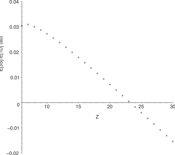
Figure 2: Minimal CI energy differences $E_{{}^{3}S^{o}}-E_{{}^{1}D^{o}}$ for the Carbon isoelectronic sequence $N=6$, $Z=6,\dots,28$. The predicted existence of a level crossing is confirmed by experiment [RJK⁺07].

We now discuss another important class of energy differences, ionization energies. The latter are defined to be (writing $E_{1}(N,Z)$ to indicate the dependence of the ground state energy on the number of electrons and the nuclear charge) $I(N,Z)=E_{1}(N-1,Z)-E_{1}(N,Z)$. Physically this corresponds to the energy required to remove one electron from a system with nuclear charge $Z$ and $N$ electrons. The calculated first ionization energies $I(N,N)$ of the minimal CI Model, in atomic units, are as follows: He 0.8477, Li 0.1912, Be 0.3237, B 0.2346, C 0.3142, N 0.3960, O 0.2708, F 0.3958, Ne 0.4141. The experimental ionization energies [Huh93] are: He 0.9036, Li 0.1980, Be 0.3426, B 0.3049, C 0.4138, N 0.5341, O 0.5000, F 0.6402, Ne 0.7925.

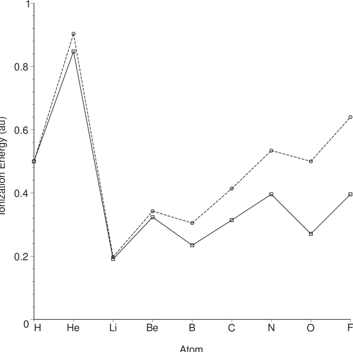
Figure 3: Experimental (dashed) and minimal CI (solid) ionization energies.

Figure 3 shows that the qualitative prediction for the ionization energies is very good when compared to experimental data. In particular, all local minimizers (H, Li, B, O), local maximizers (He, Be, N), global minimizers (Li) and global maximizers (He) are predicted correctly. This is all the more remarkable when remembering that tiny eigenvalue differences for partial differential operators on very high-dimensional spaces up to ${\mathbb{R}}^{27}$ are under consideration here.

Quantitatively, for the smaller atoms our results are comparable to (and in case of Be better than) MDHF calculations with much larger basis sets up to $20s11p$ [JAH01]. For the larger atoms the minimal dimensionality of our CI subspace finally makes itself felt, and a larger subspace (e.g. as described at the end of Section 2.4) would be needed to make the qualitative agreement quantitative.

Again, it is also instructive to compare with the PT model [FG09]. Its ionization energies, which are easily read off from the exact results of [FG09], even turn out to have the wrong sign. This shows that relaxation of orbitals is important for the description of ionization processes, and that the relaxation step (C) in the minimal asymptotics-based CI model is essential for understanding the nontrivial experimental graph in Figure 3.

Acknowledgements The research of B.G. was supported by a graduate scholarship from EPSRC. We thank P.Gill for helpful comments.

Address of authors:
Gero Friesecke
Center for Mathematics, TU Munich, Germany, gf@ma.tum.de
Benjamin D. Goddard
Mathematics Institute, University of Warwick, U.K. b.d.goddard@warwick.ac.uk

References

• [BLWW04] F. Bornemann, D. Laurie, S. Wagon, and J. Waldvogel. The SIAM 100-Digit Challenge: A Study in High-Accuracy Numerical Computing. SIAM, 2004.
• [BM04] G.L. Bendazzoli and A. Monari. A davidson technique for the computation of dispersion constants: Full CI results for Be and LiH. Chem. Phys., 306:153–161, 2004.
• [Boy50] S.F. Boys. Electronic wavefunctions. I. A general method of calculation for stationary states of any molecular system. Proc. Roy. Soc. London, A 200:542–554, 1950.
• [BT86] Ch. W. Bauschlicher and P. R. Taylor. Benchmark full configuration-interaction calculations on H2O, F, and F-. Journal of Chemical Physics, 85(5):2779–2783, 1986.
• [CNMCJ05] A. Canal Neto, E. P. Muniz, R. Centoducatte, and F. E. Jorge. Gaussian basis sets for correlated wave functions. hydrogen, helium, first- and second-row atoms. Journal of Mol. Structure: THEOCHEM, 718:219–224, 2005.
• [FG09] G. Friesecke and B.D. Goddard. Explicit large nuclear charge limit of electronic ground states for li, be, b, c, n, o, f, ne and basic aspects of the periodic table. SIAM J. Math. Analysis, to appear, 2009.
• [Fri03] G. Friesecke. The multiconfiguration equations for atoms and molecules: charge quantization and existence of solutions. Arch. Rat. Mech. Analysis, 169:35–71, 2003.
• [GBS02] F. J. Galvez, E. Buendia, and A. Sarsa. Variational Monte-Carlo calculations for some cations and anions of the first-row atoms using explicitly correlated wavefunctions. Int. J. Quantum Chemistry, 87:270–274, 2002.
• [HJO00] T. Helgaker, P. Joergensen, and J. Olsen. Molecular Electronic Structure Theory. Wiley, 2000.
• [Huh93] J. E. Huheey. Inorganic chemistry : principles of structure and reactivity. Harper Collins, 1993.
• [Hyl29] E.A. Hylleraas. On the ground state of the Helium atom. Z. Phys., 48:469, 1929.
• [JAH01] F.E. Jorge and H.M. Aboul Hosn. Gaussian basis sets for isoelectronic series of the atoms He to Ne. Chem. Phys., 264:255–265, 2001.
• [Joh05] R.D. Johnson, editor. NIST Computational Chemistry Comparison and Benchmark Database, NIST Standard Reference Database Number 101 Release 12. Aug 2005.
• [KNN08] Y.I. Kurokawa, H. Nakashima, and H. Nakatsuji. Solving the Schrödinger equation of helium and its isoelectronic ions with the exponential integral (Ei) function in the free iterative complement interaction method. Phys. Chem. Chem. Phys., 10:4486–4494, 2008.
• [KR02] J. Komasa and J. Rychlewski. Benchmark energy calculations on Be-like atoms. Phys. Rev. A, 65:042507, 2002.
• [Loe55] P.O. Loewdin. Quantum theory of many-particle systems. I. Physical interpretations by means of density matrices, natural spin-orbitals, and convergence problems in the method of configurational interaction. Phys. Rev., 97(6):1474–1489, 1955.
• [LR05] B. Leimkuhler and S. Reich. Simulating Hamiltonian dynamics. Cambridge University Press, 2005.
• [NNKI07] H. Nakatsuji, H. Nakashima, Y.I. Kurokawa, and A. Ishikawa. Solving the Schrödinger equation of Atoms and Molecules without analytical integration based on the Free Iterative-Complement-Interaction Wave Function. Phys. Rev. Lett., 99:240402, 2007.
• [RJK+07] Yu. Ralchenko, F.-C. Jou, D.E. Kelleher, A.E. Kramida, A. Musgrove, J. Reader, W.L. Wiese, and K. Olsen. NIST Atomic Spectra Database (version 3.1.2). National Institute of Standards and Technology, Gaithersburg, MD, 2007.
• [RS78] M. Reed and B. Simon. Methods of Modern Mathematical Physics. Volume IV. Dover Publications, 1978.
• [Sla30] J. C. Slater. Atomic shielding constants. Physical Review, 36(1):57–64, 1930.
• [Sla64] J. C. Slater. Atomic radii in crystals. The Journal of Chemical Physics, 41(10):3199–3204, 1964.
• [SO96] A. Szabo and N. S. Ostlund. Modern Quantum Chemistry. Dover Publications, 1996.
• [TTST94] H. Tatewaki, K. Toshikatsu, Y. Sakai, and A. J. Thakkar. Numerical Hartree-Fock energies of low-lying excited states of neutral atoms with $Z\leq 18$. Journal of Chemical Physics, 101(6):4945–4948, 1994.